Foundations of Algorithms (2015)

Appendix C Data Structures for Disjoint Sets

Kruskal’s algorithm (Algorithm 4.2 in Section 4.1.2) requires that we create disjoint subsets, each containing a distinct vertex in a graph, and repeatedly merge the subsets until all the vertices are in the same set. To implement this algorithm, we need a data structure for disjoint sets. There are many other useful applications of disjoint sets. For example, they can be used in Section 4.3 to improve the time complexity of Algorithm 4.4 (Scheduling with Deadlines).

Recall that an abstract data type consists of data objects along with permissible operations on those objects. Before we can implement a disjoint set abstract data type, we need to specify the objects and operations that are needed. We start with a universe U of elements. For example, we could have

We then want a procedure makeset that makes a set out of a member of U. The disjoint sets in Figure C.1(a) should be created by the following calls:

We need a type set_pointer and a function find such that if p and q are of type set_pointer and we have the calls

then p should point to the set containing B, and q should point to the set containing C. This is illustrated in Figure C.1(a). We also need a procedure merge to merge two sets into one. For example, if we do

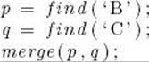
our sets in Figure C.1(a) should become the sets in Figure C.1(b). Given the disjoint sets in Figure C.1(b), if we have the call

we should obtain the result shown in Figure C.1(c). Finally, we need a routine equal to check whether two sets are the same set. For example, if we have the sets in Figure C.1(b), and we have the calls

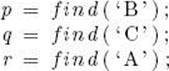
then equal(p, q) should return true and equal(p, r) should return false.

We have specified an abstract data type whose objects consist of elements in a universe and disjoint sets of those elements, and whose operations are makeset, find, merge, and equal.

Figure C.1 An example of a disjoint set data structure.

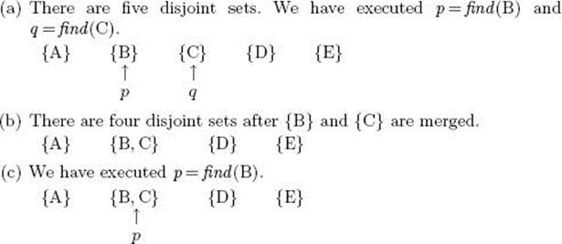
Figure C.2 The inverted tree representation of a disjoint set data structure.

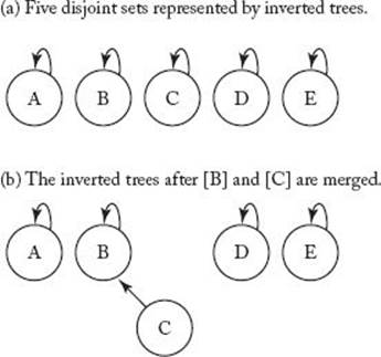
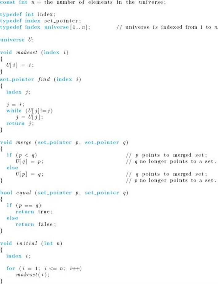
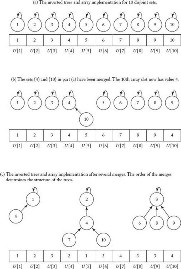
One way to represent disjoint sets is to use trees with inverted pointers. In these trees each nonroot points to its parent, whereas each root points to itself. Figure C.2(a) shows the trees corresponding to the disjoint sets in Figure C.1(a), and Figure C.2(b) shows the trees corresponding to the disjoint sets in Figure C.1(b). To implement these trees as simply as possible, we assume that our universe contains only indices (integers). To extend this implementation to another finite universe, we need only index the elements in that universe. We can implement the trees using an array U, where each index to U represents one index in the universe. If an index i represents a nonroot, the value of U [i] is the index representing its parent. If an index i represents a root, the value of U [i] is i. For example, if there are 10 indices in our universe, we store them in an array of indices U indexed from 1 to 10.

To initially place all the indices in disjoint sets, we set

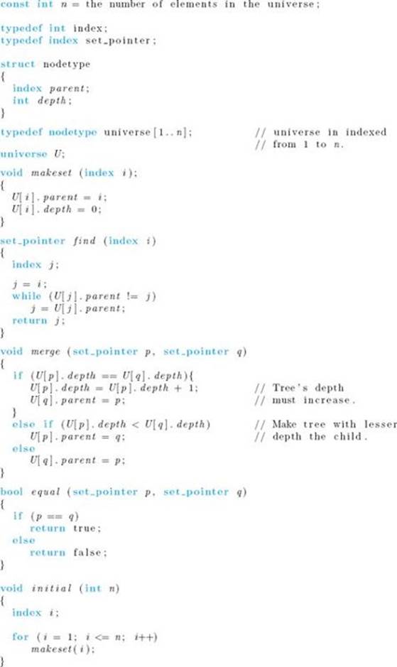
for all i. The tree representation of 10 disjoint sets and the corresponding array implementation are shown in Figure C.3(a). An example of a merge is illustrated in Figure C.3(b). When the sets {4} and {10} are merged, we make the node containing 10 a child of the node containing 4. This is accomplished by setting U [10] = 4. In general, when we merge two sets, we first determine which tree has the larger index stored at its root. We then make that root a child of the root of the other tree. Figure C.3(c) shows the tree representation and corresponding array implementation after several merges have been done. At this point there are only three disjoint sets. An implementation of the routines follows. For the sake of notational simplicity, both here and in the discussion of Kruskal’ s algorithm (see Section 4.1.2), we do not list our universe U as a parameter to the routines.

Disjoint Set Data Structure I

The value returned by the call find(i) is the index stored at the root of the tree containing i. We have included a routine initial that initializes n disjoint sets, because such a routine is often needed in algorithms that use disjoint sets.

In many algorithms that use disjoint sets, we initialize n disjoint sets, and then do m passes through a loop (the values of n and m are not necessarily equal). Inside the loop there are a constant number of calls to routines equal, find, and merge. When analyzing the algorithm, we need the time

Figure C.3 The array implementation of the inverted tree representation of a disjoint set data structure.

complexities of both the initialization and the loop in terms of n and m. Clearly, the time complexity for routine initial is in

Because order is not affected by a multiplicative constant, we can assume that routines equal, find, and merge are each called just once in each of the m passes through the loop. Clearly, equal and merge run in constant time. Only function find contains a loop. Therefore, the order of the time complexity of all the calls is dominated by function find. Let’s count the worst-case number of times the comparison in find is done. Suppose, for example, that m = 5. The worst case happens if we have this sequence of merges:

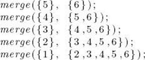
and, after each merge, we call find looking for index 6. (The actual sets were written as the inputs to merge for illustration.) The final tree and array implementation are shown in Figure C.4. The total number of times the comparison in find is done is

Generalizing this result to an arbitrary m, we have that the worst-case number of comparisons is equal to

We did not consider function equal because that function has no effect on the number of times the comparison in function find is done.

Figure C.4 An example of the worst case for Disjoint Data Structure I when m = 5.

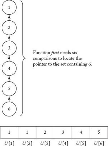
Figure C.5 In the new way of merging, we make the root of the tree with the smaller depth a child of the root of the other tree.

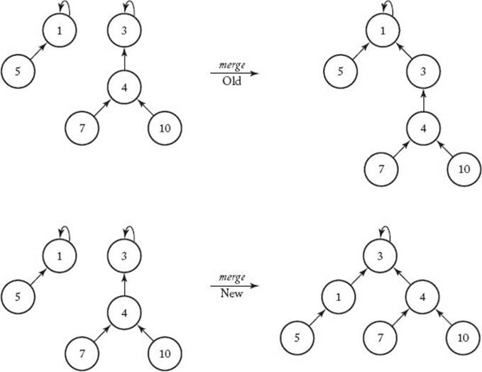
The worst case occurs when the order in which we do the merging results in a tree whose depth is one less than the number of nodes in the tree. If we modify procedure merge so that this cannot happen, we should improve the efficiency. We can do this by keeping track of the depth of each tree, and, when merging, always making the tree with the smaller depth the child. Figure C.5 compares our old way of merging with this new way. Notice that the new way results in a tree with a smaller depth. To implement this method, we need to store the depth of the tree at each root. The following implementation does this.

Disjoint Set Data Structure II

It can be shown that the worst-case number of comparisons done in m passes through a loop containing a constant number of calls to routines equal, find, and merge is in

In some applications it is necessary to locate efficiently the smallest member of a set. Using our first implementation, this is straightforward, because the smallest member is always at the root of the tree. In our second implementation, however, this is not necessarily so. We can easily modify that implementation to return the smallest member efficiently by storing a variable smallest at the root of each tree. This variable contains the smallest index in the tree. The following implementation does this.

Disjoint Set Data Structure III

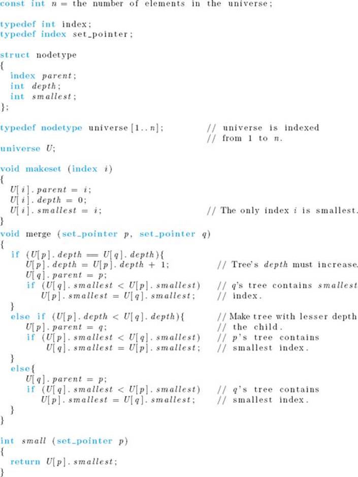
We have included only the routines that differ from those in Disjoint Set Data Structure II. Function small returns the smallest member of a set. Because function small has constant running time, the worst-case number of comparisons done in m passes through a loop containing a constant number of calls to routines equal, find, merge, and small is the same as that of Disjoint Set Data Structure II. That is, it is in

Using a technique called path compression, it is possible to develop an implementation whose worst-case number of comparisons, in m passes through a loop, is almost linear in m. This implementation is discussed in Brassard and Bratley (1988).