Macs All-in-One For Dummies, 4th Edition (2014)
Book V. Taking Care of Business
Chapter 5. Crunching with Numbers
In This Chapter
![]() Getting to know the Numbers spreadsheet
Getting to know the Numbers spreadsheet
![]() Creating a spreadsheet
Creating a spreadsheet
![]() Using sheets
Using sheets
![]() Working with tables and charts
Working with tables and charts
![]() Polishing a spreadsheet
Polishing a spreadsheet
![]() Printing and sharing your spreadsheet
Printing and sharing your spreadsheet
Numbers is a spreadsheet application designed to help you manipulate and calculate numbers for a wide variety of tasks, such as balancing a budget, calculating a loan, and creating an invoice. The Numbers application also lets you create line, bar, and pie charts that help you analyze your data graphically. What’s more, Numbers offers organizational and layout capabilities that you won’t find in other spreadsheet apps.
In this chapter, we explain the parts of a spreadsheet; then we explain how to create a new spreadsheet on your Mac or iCloud, or open an existing spreadsheet created in a different application. We show you how to work with your data on a spreadsheet, including setting up tables, entering data, and using formulas. We give you some tips for personalizing a spreadsheet to make it aesthetically pleasing. At the end of the chapter, we go over printing and sharing your spreadsheet, even if the person you want to share with doesn’t use Numbers.
 Numbers is part of the iWork suite. If you bought a new Mac after November, 2013, iWork apps are included. If you have an older Mac, you can purchase and download Numbers from the App Store for $19.99. If you have an iPhone, iPad, or iPod touch, the iOS version of Numbers lets you create and work on documents on those devices when you don’t have your Mac handy. And, by saving your Numbers documents to iCloud, you can open them on the iCloud website on computers running Windows or Linux.
Understanding the Parts of a Numbers Spreadsheet
The Numbers window is divided into two main sections: the sheet and the Format/Filter pane. You place charts, tables, data, functions, and even graphics and media on the sheet. The Format pane is where you apply styles and color to the fonts and data you select in the worksheet, and the Filter pane is where you establish criteria to sort data on tables. Other things you can see on the Numbers window are
· Toolbar: Across the top is the toolbar, which has buttons for frequently performed tasks.
· Sheet tabs: As you add new sheets to the file, tabs appear across the top, which you click to move from one sheet to another.
· Rulers: If you choose View⇒Show Rulers, you see rulers above and to the left of the active sheet, which help you determine the final size of your spreadsheet, especially if you want to print it.
A sheet may have zero or more tables, which are distinct gridworks comprising rows (identified by incremental numbers down the left margin) and columns (in alphabetical order by a letter at the top). The intersection of a row and column is a cell, and that’s where you type and store numbers, text, and formulas, as shown in Figure 5-1. A cell has the coordinates of the row and column; E4, for example, is the intersection of the fifth column (E) and the fourth row (4).
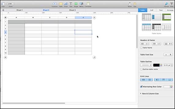
Figure 5-1: The parts of a Numbers window and table.
Besides the mundane-but-fundamental cells that form the backbone of any spreadsheet, you can also place the following eye-catching (and useful) items in your sheets by clicking the buttons on the toolbar, as shown in Figure 5-2:
· Table: A table consists of rows and columns that can contain words, numbers, calculated results, or a combination of these types of contents.
· Chart: A chart displays data stored in a table. Common types of charts are line, bar, pie, and column. With Numbers, you can build two-axis and mixed charts as well as 2D, 3D, and interactive charts.
· Text: Text serves both decorative and informative functions. In a text box, you type and store text independent of the rows and columns in a table.
· Shape: Choose from three line styles and a dozen shapes to add pizazz to your sheet.
· Media: Add photos, music, or movies to your sheet.
· Comment: Comments are particularly useful when you share your sheets because others can give you feedback without changing the sheet itself.
Figure 5-2: A sheet can have tables, charts, text boxes, and images.
Putting together a spreadsheet is a simple process. The following list points out the basic steps:
1. Start with a sheet.
When you create a new Numbers document, either from scratch or by using a template, Numbers automatically creates one sheet with one table on it. Your job is to fill that table with data — although you could delete it if you want to use that sheet as a cover page. Add more tables — yes, a sheet can hold multiple tables — or start spicing up your data presentation with charts or pictures. (More on that later.)
2. Fill a table with numbers and text.
After setting up at least one table on a sheet, you can move the table around on the sheet and/or resize it. When you’re happy with the table’s position on the sheet and the table’s size, you can start entering numbers into the table’s rows and columns. Add titles to the rows and columns to identify what those numbers mean, such as August Sales or Car Payments.
3. Create formulas and use functions.
After you enter numbers in a table, you’ll want to manipulate one or more numbers in certain ways, such as totaling a column of numbers. Numbers offers 250 predefined functions to take your numbers or text and calculate a result, such as how much your company made in sales last month or how a salesperson’s sales results have changed.
Functions are pre-loaded in Numbers and use one or more variables to calculate a result. You write formulas. Both are mathematical expressions that not only calculate useful results, but they also let you enter hypothetical numbers to see possible results. For example, if every salesperson improved her sales results by 5 percent every month, how much profit increase would that bring to the company? By typing in different values, you can ask, “What if?” questions with your data and formulas.
4. Visualize data with charts.
Just glancing at a dozen numbers in a row or column might not show you much of anything. By turning numeric data into line, bar, or pie charts, Numbers can help you spot trends in your data.
5. Polish your sheets.
Most spreadsheets consist of rows and columns of numbers with a bit of descriptive text thrown in for good measure. Although functional, such spreadsheets are boring to look at. That’s why Numbers gives you the chance to place text and images on your sheets to make your information (tables and charts) compelling. You can even add audio effects!
Creating a Numbers Spreadsheet
To help you create a spreadsheet, Numbers provides 31 templates that you can use as-is or modify. Templates contain preset tables with formulas, which calculate the task at hand. For example, in the Savings Tracker template, you enter your goal, the length of time for your investment, and the interest rate, and then the template calculates how much you have to save each month to reach your goal. Changing those values changes the results.
Templates also have predefined font styles and color schemes. You can alter anything you want in a template — tables, charts, colors — but finding a template that is close to what you want to do gives you a head start. That way, you don’t have to spend time designing, so you can concentrate on your figures.
 If you prefer, use the Blank template to create a spreadsheet (one sheet with one table) from scratch. If you design a particularly useful spreadsheet, you can save it as a custom template (by choosing File⇒Save as Template).
Creating a new spreadsheet with a template
To create a spreadsheet based on a template, follow these steps:
1. Double-click the Numbers icon in Launchpad or click the Numbers icon on the Dock (or choose File⇒New on the menu bar if Numbers is already running).
The icon looks like a 3D bar chart. When you click it, one of the following happens:
· If you didn’t turn on Numbers in iCloud, the Themes chooser opens.
· If you turned on Numbers in the Documents & Data section of iCloud (see Book I, Chapter 3), you have to first choose where you want to work: iCloud or Mac. When you open Numbers to create a new document or work on an existing one, you have to click iCloud or On My Mac to choose where you want to save your new document (or to find an existing document) and then click New Document to open the Choose a Theme dialog, as shown in Figure 5-3.
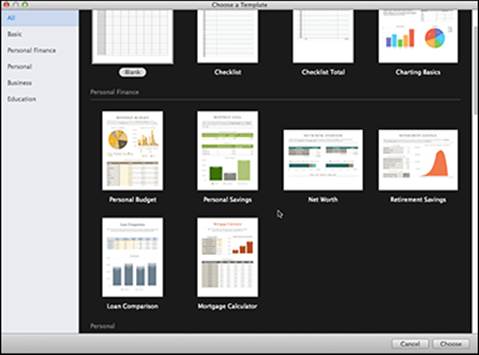
Figure 5-3: Templates are organized in categories, such as Personal or Business.
2. Click a template category in the list on the left (or click All if you want to see all 31 templates).
Choose a template that is closest to what you want to do: for example, a household budget or a workout tracker.
3. Double-click the template that you want to use, or click the template you like in the main pane. Then click the Choose button.
Numbers opens your chosen template.
If you want to start with a blank spreadsheet, click Blank which is the first template under Basic.
4. Choose File⇒Save.
The Save As dialog opens.
5. Type a name for your spreadsheet and choose the folder where you want to store it on your Mac or save it to iCloud.
Opening an existing file
If you’re working on a Numbers document on one source (such as your Mac) and you want to open a document from another source (such as iCloud or an external drive), choose File⇒Open, and do one of the following:
· Click iCloud, click one of the documents in the list, and then click Open.
You need an Internet connection to work on iCloud documents.
· Click On My Mac, scroll through the directories and folders to find an existing document you want to work on, click it, and then click Open. Choose On My Mac to access external drives and servers, too.
You might have spreadsheets that were created in a different application (such as Microsoft Excel, Quicken Open Financial Exchange [OFX], or AppleWorks 6), or you may have raw data that you want to bring into Numbers (such as comma-separated value [CSV] or tab-delimited text). You can open the file in Numbers, and Numbers will create sheets and tables with the data supplied. To open a non-Numbers file, drag the file you want to open over the Numbers icon on the Dock or follow the steps outlined earlier for opening a file via On My Mac.
Working with Sheets
Every Numbers spreadsheet needs at least one sheet, although you can have many (refer to Figure 5-1) . A sheet acts like a limitless page that can hold any number of tables, charts, and other objects. You want to use sheets to organize the information in your document, such as using one sheet to hold January sales results, a second sheet to hold February sales results, and a third sheet to hold a line chart that shows each salesperson’s results for the first two months.
To help organize your sheets, Numbers stores the names of all your sheets in the tabs at the top of the sheet. Clicking the disclosure triangle on the right end of a sheet tab opens a list of all tables and charts stored on that particular sheet, along with options for copying, deleting, or renaming the sheet, as shown in Figure 5-4.
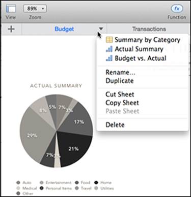
Figure 5-4: View a sheet’s elements.
To view the contents of a specific sheet, click that sheet name at the top of the sheet. To view a particular table or chart, find the sheet that contains that table or chart. Then click that specific table or chart.
Adding a sheet
You can always add another sheet. When you add a sheet, Numbers creates one table on that sheet automatically. To add a sheet, choose one of the following:
· Choose Insert⇒Sheet from the menu bar.
· Click the Add Sheet icon (a + sign) that appears at the far left of the row of sheet tabs.
Deleting a sheet
If you need a sheet to go away, clear out, disappear, whatever, you can delete it.
 When you delete a sheet, you also delete any tables or charts stored on that sheet.
To delete a sheet, hover the cursor over the right end of the tab for the sheet you want to delete. Click the disclosure triangle when you see it, and then choose Delete from the pop-up menu (refer to Figure 5-4).
Adding or removing a table
As we mention earlier, a sheet can hold one or more tables, and the data you put in a table can be used as data references for charts you add to sheets. When you add a table, it uses the color scheme you choose and the typefaces associated with the template you’re using, but it’s empty — you have to input the data. Here, we show you how to add and format tables and then delve into how to use them to manipulate and display your data.
To add a table, follow these steps:
1. Click the tab for the sheet where you want to insert the table.
2. Click the Table icon on the toolbar and click the left and right arrows to flip through the color selection. Click the table you like.
The table appears on your slide.
To remove a table, click the Resize button and then press Delete.
Resizing a table
You have a variety of options for changing the size of your table:
· Resize handles: Click the table and then click the Select Table button in the upper-left corner. Drag the handles around the edges to resize the table. This doesn’t add rows and columns, just proportionately changes the table size.
· Resize corner: Click inside the table, and then click and drag the button in the bottom-right corner to add or remove columns and rows, and define the overall size and shape of your table.
· Adding row/column button: Click the Add button (two parallel lines in a circle) at the bottom-left corner to add rows or at the upper-right corner to add columns. Rows and columns are added to the table automatically.
· Inserting or delete a row or column: Hover the cursor by the row or column identifier (letters for columns, numbers for rows) before or after where you want to insert a row or column until you see a disclosure arrow. Click the arrow to open a menu that gives you choices to insert a row or column before or after the one you selected. You can also delete or hide the row or column you selected.
Delete multiple columns or rows by highlighting those column or row headings, clicking the Table menu, and then choosing Delete Columns or Delete Rows.
If you click the disclosure arrow of column A or B or row 1 or 2, you also have choices to insert header rows or columns or to convert the selected row or column into a header row or column. (See the Inserting headers and resizing rows and columns section for more information.)
· Adjusting row height or column width: Follow the steps for inserting but choose Fit Height/Width to Content adjust the height or width of the row or column to accommodate the contents of the cells in that row or column. Or, click the column or row and then hover the cursor over one of the edges of the row or column header until the cursor becomes a double-sided arrow. Click and drag the cursor/arrow to adjust the height or width of the row or column.
Changing the appearance of a table
Click the Format button on the toolbar to see the tools you can use to edit the appearance of your table. Select the cells, rows, or columns you want to edit, and click the tab of the Format pane for the things you want to change:
· Table: Use this tab’s menus and buttons to adjust the color, font size, grid lines, and number of header and footer cells. These changes affect the entire table.
· Cell: Make changes to the cells, rows, or columns you select either singly or in multiples. Define how the data is formatted, such as currency or percentage, and assign fill and border colors and styles.
· Text: Define the text color, style, and alignment of text in selected cells, rows, or columns.
· Arrange: Reposition the table in relation to other objects on the sheet or align it on the sheet itself.
Inserting headers and resizing rows and columns
Headers are the first rows and columns of your table, where you usually type the names of the rows and columns. Footers are the final rows of the table, where you can repeat header names in particularly large tables. You can have header rows and columns that span up to five rows or columns, which is a handy way to use titles and subtitles for each row or column. Another way to insert header rows and columns is the following:
1. Click the table, click the Format button on the toolbar, and then click the Table tab of the Format pane.
2. In the Headers & Footer section, use the pop-up menus to choose the number of row and column headers and column footers you want, up to five for each.
3. To make your header rows and columns stay put while you scroll through the rest of your table, click Freeze Header Row/Column in the pop-up menu.
To insert header rows or columns after you already have data in your table, follow these steps:
1. Click a cell in one of the header rows or columns, either before or after where you want to insert another header row or column.
2. Click the Table menu and choose from the following:
· Add Header Row Above: Inserts an additional header row directly above the selected cell
· Add Header Row Below: Inserts an additional header row directly below the selected cell
· Add Header Column Before: Inserts an additional header column to the left of the selected cell
· Add Header Column After: Inserts a new column to the right of the selected cell
3. (Optional) Click a cell and use the menus in the Row & Column Size section to give a specific size to the row height or column width, or click the Fit button to have Numbers make automatic adjustments based on the amount of data in the cells in that row or column.
To emphasize the header rows and columns and footers and make them stand out from the contents of the table, you can outline single cells — or the entire row or column — with a border and/or fill the cells with a background color. Select the cells you want to emphasize and then do the following:
1. Click the Cell tab in the Format pane (click the Format icon on the toolbar if you don’t see the Format pane).
2. Click the disclosure triangle next to Border to open the border options.
1. Click the border style button (it looks like a paintbrush on a line) and choose a border style and the parts of the cells you want to apply it to.
If you select one cell in the table and then choose the four-sided border, the four sides of that one cell will have the border.
If you select several cells, and then choose the four-sided border, the border surrounds the group but the lines between the cells remain unchanged.
If you want to add a border around all the selected cells, choose the border style that has both the outline and the inner lines emphasized.
2. Click the pop-up menu beneath the word Border to change the border style from line to dash or dot.
3. Use the up and down arrows beneath that pop-up menu to change the thickness of the border.
4. Click the color swatch to choose a standard color or click the button next to the swatch to open the color pickers and choose a color from there.
3. Click the disclosure triangle next to Fill to add a background color to the headers or footers.
1. Click the color swatch to choose a standard color or click the button next to the swatch to open the color pickers and choose a color from there.
2. Click the Color Fill pop-up menu to choose the type of fill, such as Gradient.
Typing Data into Tables
Now we get into the numbers part of Numbers. You need to know about the three types of data you can store inside a table: numbers, text, and formulas. You can also store images in a cell, which doesn’t work as data per se but is useful to create documents such as an inventory or real estate listing.
We give you details about working with each type of data in the next three sections. However, in summary, to type anything into a table, follow these steps:
1. Select a cell by clicking it or by pressing the arrow keys.
2. Type a number, text, or formula.
If you want to use a predefined function or create a formula of your own, type an equal sign (=) in the cell. The Function panel opens on the right side of the window.
3. Press Return to select the cell below, press Tab to select the cell to the right, or click any cell into which you want to type new data.
4. Repeat Steps 2 and 3 for each additional formula or item of data you want to type into the table.
Formatting numbers and text
When you type a number in a cell, the number will look plain — 45 or 60.3. To make your numbers more meaningful, you should format them. For example, the number 39 might mean nothing, but if you format it to appear as $39.00, your number now clearly represents a dollar amount.
To format numbers, follow these steps:
1. Click to select one cell or click and drag to select multiple cells.
Numbers draws a border around your selected cell(s).
If you select empty cells, Numbers remembers the assigned format and automatically formats any numbers you type into those cells in the future.
2. Click the Format button on the toolbar, and then click the Cell tab of the Format pane.
3. Choose how you want the data to appear in the Data Format pop-up menu, as shown in Figure 5-5.
Each choice has options that appear in the Format pane:
· The numeric choices have submenus with further choices, such as how many decimals or the currency symbol.
· When cells are formatted as Text, numbers have no numeric values. This is useful for typing in zip codes and phone numbers.
· The Date & Time and Duration choices offer formatting options such as spelling out the month or using a number. Here, too, numbers are considered text.
· The last set of choices are neither numeric nor text but instead let you create data entry cells that require an action, such as clicking to place a check mark in the box or limit your choices, such as a pop-up menu. (See “Formatting data entry cells,” later in this chapter).
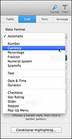
Figure 5-5: Data looks, and works, differently depending on how it’s formatted.
To add color to your cells and/or definition to them, click the disclosure triangles next to the Fill and Border options. Choose the options you want from the pop-up menus, as shown in Figure 5-6.
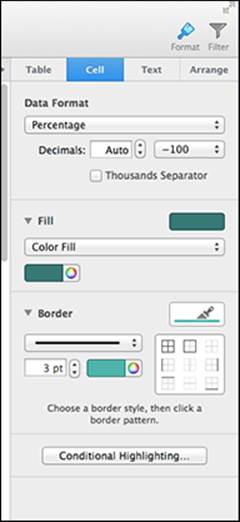
Figure 5-6: Add background colors and borders to cells.
The cells automatically change as you try different effects.
· Fill puts a color, a gradient, or an image behind characters typed in the cell. Depending on the choice, you’re presented with tools for choosing the color, the spectrum and direction (gradient), and scaling (image).
· Border surrounds your cell(s) with a line; define the width and color, and choose whether you want a border around each cell or around the group of cells or only on one side or in between.
· Click the Colors icon in either section to change the color of the fill or border. The color block opens a chooser that displays colors used in the theme; the color wheel opens the Colors window.
1. Click the color picker you prefer: Wheel, (which is the default), Slider, Palette, Spectrum, or Crayons.
2. Click the desired color in the color picker that appears in the Colors window.
3. (Optional) In the color picker, make the color lighter or darker by dragging the slider on the right up and down.
4. (Optional) In any of the color pickers, adjust the opacity by dragging the opacity slider left and right or type in a precise percentage in the text box to the right.
5. When you have a color you like, drag the color from the color box at the top to the color palette at the bottom. Your color is saved in the palette for future use.
6. Click the red Close window button or choose View⇒Close Colors.
To format the style of the characters in the selected cell(s) — whether they’re formatted as numbers, text, or data entry — click the Text tab and then the Style button in the Format pane.
· To use a different font in the theme: Click the Paragraph Styles menu and choose a different font.
· To change the font style: In the Font section, scroll through the Family menus to select the options you want.
The Family menu shows the fonts as they are to help you imagine your presentation using that font.
Click the font when you find it, and then click the Typeface, Size, and Style menus and buttons to make those changes to your type.
Change the font color by clicking the color wheel and following the steps mentioned previously.
· To choose how you want your text to appear in the cell: Click the horizontal and vertical Alignment buttons. Cells that will contain numbers usually have right alignment, and text in header cells is often centered.
If you’re working with text, in a text box, you can select it and format the line and paragraph spacing, such as 1.5 line spacing and double-spacing between paragraphs. You can also create a bulleted or numbered list with the options in the Bullets & Lists section.
Typing formulas
The main purpose of a table is to use the data (numbers, textual data, dates, and times) you store in cells to calculate a new result, such as adding a row or column of numbers. To calculate and display a result, you need to store a formula in the cell where you want the result to appear.
Numbers provides three ways to create formulas in a cell:
· Quick Formula
· Typed formulas
· Advanced functions
Using Quick Formula
To help you calculate numbers in a hurry, Numbers Quick Formula feature offers a variety of formulas that can calculate common results, such as
· Sum: Adds numbers
· Average: Calculates the arithmetic mean
· Minimum: Displays the smallest number
· Maximum: Displays the largest number
· Count: Displays how many cells you select
· Product: Multiplies numbers
To use a Quick Formula, follow these steps:
1. Click the empty cell at the bottom or to the right of cells that contain the numbers you want to operate the function on.
2. Click the Function icon on the toolbar or choose Insert⇒Function on the menu bar.
3. From the pop-up menu (or sub-menu) choose Sum, Average, Minimum, Maximum, Count, or Product.
Numbers displays your calculated results.
Typing a formula
Quick Formula is handy when it offers the formula you need, such as when you add up rows or columns of numbers with the Sum formula. Often, however, you need to create your own formula.
Every formula consists of two parts:
· Operators: Perform calculations, such as addition (+), subtraction (–), multiplication (*), and division (/)
· Cell references: Define where to find the data to use for calculations
A typical formula looks like this:
= A3 + A4
This formula tells Numbers to take the number stored in column A, row 3 and add it to the number stored in column A, row 4.
To type a formula, follow these steps:
1. Click (or use the arrow keys to highlight) the cell where you want the formula results to appear.
2. Type =.
The Formula Editor appears.
3. Click a cell that contains the data you want to include in your calculation.
4. Type an operator, such as * for multiplication or / for division.
5. Click another cell that contains the data you want to include in your calculation.
6. Repeat Steps 4 and 5 as needed.
7. Click the Accept (or Cancel) button in the Formula Editor when you’re done.
Numbers displays the results of your formula. If you change the numbers in the cells you define in Steps 3 and 5, Numbers calculates a new result instantly.
For a fast way to calculate values without having to type a formula in a cell, use Instant Calculations. Just select two or more cells that contain numbers, and you can see the results in the Instant Calculations results tabs along the bottom of the Numbers window, as shown in Figure 5-7. You can change the types of results you see in the Instant Calculations Results tabs by clicking the Action button (it looks like a gear) and selecting the functions you want to see from the pop-up menu.
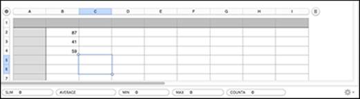
Figure 5-7: Instant Calculations can show results without typing a formula first.
Using functions
Typing simple formulas that add or multiply is easy. However, many calculations can get more complicated, such as trying to calculate the amount of interest paid on a loan with a specific interest rate over a defined period.
To help you calculate commonly used formulas, Numbers provides a library of 250 functions, which are prebuilt formulas that you can plug into your table and define what data to use without having to create the formula yourself.
To use a function, follow these steps:
1. Click (or use the arrow keys to highlight) the cell where you want the function results to appear.
Some functions operate on data typed into the cell where the function is inserted. For example, if you insert the sine function, the sine of numbers you type into that cell will be calculated. Other functions use data in several cells to calculate a result, such as depreciation, which uses original cost, time in service, and some other business-y information. That type of information must be typed into the cells that the function refers to in order for it to work.
2. Press the equal (=) key.
The Formula Editor appears, and the Functions pane opens, as shown in Figure 5-8.
You can move the Formula Editor if you move the pointer to the left end of the Formula Editor. When the pointer turns into a hand, click and drag the Formula Editor to a new location so it doesn’t hide the cells you’re working on.
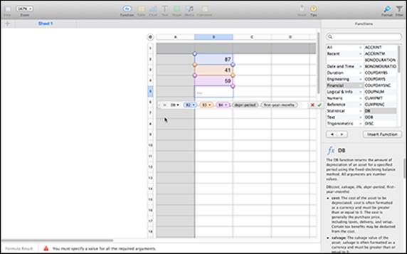
Figure 5-8: The Functions pane displays all available functions in Numbers.
3. Choose the type of function you want from the left column (or click All), and then scroll through the functions on the right and click the one you want to insert.
A definition for the selected function is shown at the bottom of the pane, along with an explanation of the types of data needed to complete the operation and an example of how it works.
4. Click the Insert Function button.
The Formula Editor now contains your chosen function.
5. Edit the formula by typing the cell names (such as C4) or clicking the cells that contain the data the function needs to calculate.
6. Click the Accept (check mark) or Cancel (x) button on the Formula Editor.
Numbers shows your result.
Choose View⇒Show Formula List to see a list of all the formulas used in a spreadsheet. You can also see the formulas used in templates in this way.
Formatting data entry cells
After you create formulas or functions in cells, you can type new data in the cells defined by a formula or function and watch Numbers calculate a new result instantly. Typing a new number in a cell is easy to do, but sometimes a formula or function requires a specific range of values. For example, if you have a formula that calculates sales tax, you may not want someone to enter a sales tax more than 10 percent or less than 5 percent.
To limit the types of values someone can enter in a cell, you can use one of the following methods, as shown in Figure 5-9:
· Sliders: Users can drag a slider to choose a value within a fixed range.
· Steppers: Users can click up and down arrows to choose a value that increases or decreases in fixed increments.
· Pop-up menus: Users can choose from a limited range of choices.
You can also format the cell with a check box or star rating, as shown in Figure 5-9.
Formatting a cell with a slider or a stepper
Using a slider or stepper is useful when you want to restrict a cell to a range of values, such as 1–45. The main difference is that a slider appears next to a cell, whereas a stepper appears inside a cell.
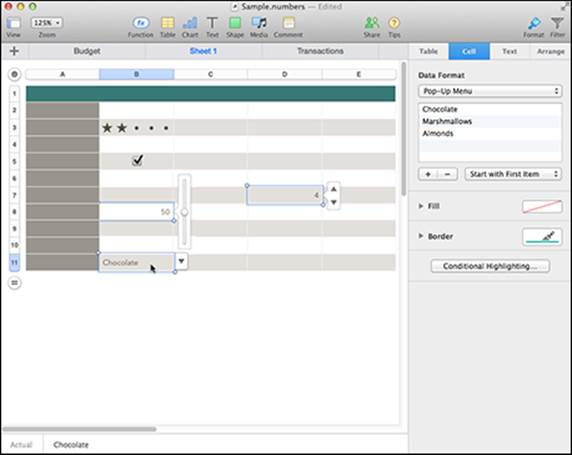
Figure 5-9: Sliders, steppers, and pop-up menus restrict the types of values a cell can hold.
To format a cell with a slider or stepper, follow these steps:
1. Click a cell that you want to restrict to a range of values.
2. Click the Format button on the toolbar, and then click the Cell tab of the Format pane.
3. Choose Slider or Stepper from the Data Format pop-up menu.
4. Enter the minimum acceptable value.
5. Enter the maximum acceptable value.
6. Enter a value in the Increment text box to increase or decrease by when the user drags the slider or clicks the up- and down-arrows of the stepper.
7. Use the Format and Decimals menus to edit the displayed number.
Numbers displays a slider next to the cell. Users have a choice of typing a value or using the slider to define a value. If you choose a value outside the minimum and maximum range defined in Steps 3 and 4, the cell won’t accept the invalid data.
Formatting a cell with a pop-up menu
A pop-up menu restricts a cell to a limited number of choices. To format a cell with a pop-up menu, follow these steps:
1. Repeat Steps 1 and 2 for inserting a slider or stepper (see the preceding section).
2. Click the list box under the Data Format pop-up menu.
3. Click the plus (+) sign button to add an item to the pop-up menu associated with the cell, and then type in the number or text you want added.
Repeat to add other items.
4. To remove an item from the list, click the item and then click the minus (–) sign button.
Repeat to delete other items.
5. Choose Start with First Item or Start with Blank from the pop-up menu next to the add/delete items buttons.
This determines what will be shown in the cell.
Numbers displays a pop-up menu that lists choices when users click that cell.
You can also set a conditional highlight so that if your data meets a certain criterion or condition, Numbers will highlight the number or text in a color you want. Say you create a spreadsheet to track office supply inventory, and you want to know when you have fewer than five black pens. Set the conditional formatting of the cell to “less than or equal to 5.” Then, when there are five pens or fewer, the cell changes color. Now, at a glance, you see pertinent information. To use conditional formatting, follow these steps:
1. Select the cell(s) where you want to use conditional formatting.
2. Click the Format button on the toolbar, and then click the Cell tab of the Format pane.
3. Click the Conditional Highlighting button at the bottom of the pane.
You may have to scroll to find it.
4. Click the Add a Rule button.
The Conditional Formatting window opens.
5. Peruse the tabs and select the rule you want to use, as shown in Figure 5-10.
A field appears where you can type in a value.
· If you want to refer to another cell: Click the blue circle on the right end of the field and type in a cell reference. Or, click the cell in your sheet, and its reference appears in the field.
· To change the value: Click in the field and press the Delete key, and then type another value or enter a different cell reference.
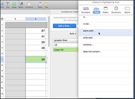
Figure 5-10: Numbers formats cells that meet Conditional Formatting criteria.
6. Click the pop-up menu to format how you want the data highlighted.
The sample box shows how the cell will appear if the data in it meet the conditional rule you set.
7. (Optional) To add another rule, repeat Steps 4–6.
8. (Optional) To delete a rule, click the trash can icon that appears when you hover the cursor to the right of the rule name.
9. (Optional) To rearrange the order of the rules, hover the cursor to the left of the rule name and click and drag the Rearrange button (it looks like three horizontal lines).
10. Click Done.
Sorting data
When you enter your data, you don’t always do so in the order you want to see it. For example, to track invoices, you create a column for each piece of data, such as invoice number, date of purchase, customer name, and total, and then you enter the data from a stack of invoices so each row holds the data for one invoice. You may enter the data by invoice number first but then want to sort by customer name to see which customers have more than one outstanding invoice or by total to see who spent the most. You can sort the data by one of those columns. Here’s how you do it:
1. Click the table you want to sort or select a group of cells you want to sort.
2. Hover the cursor over the column indicator (the letters) that you want to use to define the sort.
3. Click the disclosure triangle that appears to open the pop-up menu.
4. Select Sort Ascending or Sort Descending to establish the order in which you want the data.
Numbers will sort your data by the column you chose.
Deleting data in cells
If you ever want to delete data in a cell, Numbers provides two ways:
· Delete data but retain any formatting.
· Delete data and formatting.
To delete data but retain any formatting, follow these steps:
1. Select one or more cells that contain data you want to delete.
2. Press Delete or choose Edit⇒Delete from the menu bar.
To delete both data and formatting in cells, follow these steps:
1. Select one or more cells that contain data and formatting you want to delete.
2. Choose Edit⇒Clear All from the menu bar.
Adding a chart
Charts are a graphical representation of data. Before you add a chart to your sheet, create a table and enter the data you want the chart to represent. Then, do the following:
1. On the table where you input the data for your chart, click and drag to select the data, including row and column headers.
2. Click the Chart icon on the toolbar and then click the left and right arrows to flip through the color selection. First, click a tab for the type of chart you want — 2D, 3D, or Interactive — and, then choose the chart you want.
The chart with your data appears on your sheet.
If the data is on one sheet but you want to place the table on another sheet, do the following (you can also use these steps to create charts on the same sheet, if you want):
1. Click that sheet where you want to place the chart.
2. Click the Chart icon on the toolbar and then click the left and right arrows to flip through the color selection. First, click a tab for the type of chart you want — 2D, 3D, or Interactive — and, then choose the chart you want.
3. Click the Add Chart Data button.
4. Click the sheet that holds the data.
5. Click and drag to select the cells, including headers, that contain the data you want in the chart.
6. Click the Done button.
The data selected from the table flows into the chart on the other sheet.
Interactive charts are created the same way as 2D or 3D charts. Here’s the difference. Rather than see, for example, eight columns that represent two types of data for four months, you see two columns at a time, and clicking the playback arrows animates the data.
7. Click Format on the toolbar and then go through the tabs of the Format pane to edit the appearance and position of the chart and data:
· Chart gives you tools for changing the colors and fonts of the chart, as well as adding special effects such as shadow or opacity and a title and/or legend. At the bottom of the panel is the Chart Type menu. Click to change to a different type of chart, and any data you entered will appear on the new type.
· Axis (all but pie charts) lets you name the axes and change the scale. Here you also find the menus for defining the value labels with percentage, currency, or others.
· Series (all but pie charts) offers menus for naming the value labels.
· Wedges (only pie charts) shows check boxes and menus for adding labels and defining the value data format. You can move the labels off the chart itself and separate the pieces of the pie by setting a greater distance from center with the respective slider bars.
· Arrange lets you reposition the chart in relation to other objects on the slide or align it on the sheet itself. This doesn’t change parts of the chart.
· Axis/Wedge Labels lets you can define the label (number, percentage, and so on) and also change the font family, size, style, and color. Double-click any of the text on the chart, and the Axis or Wedge Labels tab appears in the Format pane.
8. (Optional) To remove a chart, click it and then press Delete.
You can also use the Numbers menu to add objects to your slides; choose Insert⇒Table/Chart/Shape/Line and then choose the specific type from the submenu that opens.
Naming sheets, tables, and charts
Numbers gives each sheet, table, and chart a generic name, such as Sheet 2, Table 1, or Chart 3. To help you better understand the type of information stored on each sheet, table, and chart, use more descriptive names, especially when you add multiple tables and charts. The sheet name appears on the sheet tab, and table and chart names appear when you click the disclosure triangle on the sheet tab.
To name a sheet, double-click the name on the sheet tab to select it and type a new name, or choose Rename from the sheet tab pop-up menu and then rename it.
Although you don’t have to have a name for your charts and tables, it does help if you have more than one chart or table on a sheet. To name a table or chart, double-click the placeholder text to type a name for the table or chart. If you don’t see the placeholder text, click the table or chart, and then click the Format button on the toolbar. Click the Table or Chart tab in the Format pane, and then select the check box next to Table Name or Title (for charts). Click the Table tab and Outline Table Name to put a box around the table name.
To move a table or chart from one sheet to another, click the table or chart and choose Edit⇒Cut. Click the sheet you want to move the table or chart to, and then choose Edit⇒Paste. Data and calculations remain unchanged. Click and drag the table or chart to the position you want on the sheet.
Making Your Spreadsheets Pretty
Tables and charts are the two most crucial objects you can place and arrange on a sheet. However, Numbers also lets you place text boxes, shapes, and pictures on a sheet. Text boxes can contain titles or short descriptions of the information displayed on the sheet. Shapes can add color or indicate navigational cues, such as arrows. Photos can make your entire sheet look more interesting, or they may be the focus of your sheet if you’re creating an inventory.
Click the Table tab in the Format pane, and choose alternating Row Color to have that effect in your table. The colors will reflect those of the theme you chose, but you can change them with the color tool, which we explain in detail in the “Formatting numbers and text” section.
Adding a text box
To add a text box to a sheet, follow these steps:
1. Click the sheet tab to which you want to add the text box.
Numbers displays your chosen sheet and any additional objects that may already be on that sheet, such as tables or charts.
2. Click the Text icon (T) on the toolbar.
A text box appears on the sheet.
3. Double-click in the text box and type any text that you want to appear in the text box. Press Return to type text on a new line.
While you type, your text box lengthens to accommodate your text. You can widen the text box by clicking and dragging the handles on its sides.
4. (Optional) Select any text and choose any formatting options from the Format pane, as we explain earlier for formatting text in tables and cells.
Adding media
To add a photo, a movie, or audio file such as a TIFF, JPEG, or AIFF, to a sheet, follow these steps:
1. Click the sheet tab to which you want to add media.
2. Click the Media icon on the toolbar.
The Media Browser appears.
3. Do one of the following:
· Photo: Click the Photos tab, scroll through the thumbnails, and click one you want to insert.
· Music: Click the Music tab, and then click the song or spoken audio you want to add.
· Movies: Click the Movies tab, and then click the movie you want to insert.
Numbers displays your chosen image or movie on the sheet. If you added audio, a play icon indicates that. You can move the media around the sheet, resize photos and movies with the resizing handles, and use the editing tools of the Format pane to add borders or fills.
4. (Optional) To delete inserted media, click it and press Delete.
If you want to use an image as a background for a cell or group of cells, select the cells and then use the Fill tool of the Format pane.
Sharing Your Spreadsheet
You put a lot of effort into making your spreadsheet presentable. When you’re ready to actually present it, you can share your spreadsheet with others by printing it or saving it as a file for electronic distribution.
Printing a spreadsheet
In other spreadsheet applications, it’s not uncommon to print your spreadsheet and chart only to find that part of your chart or spreadsheet is cut off by the edge of the paper. To avoid this problem, Numbers displays a Content Scale, which lets you magnify or shrink an entire sheet so it fits and prints perfectly on a page.
To shrink or magnify a sheet to print, follow these steps:
1. Click the sheet tab you want to print.
2. Choose File⇒Print.
Numbers displays a page and shows how the charts and tables on your sheet will print. If you can’t see the whole page, change the view to 75% or 50% with the pop-up magnifying menu to see the borders of the page and where your tables and objects lie, as shown in Figure 5-11.
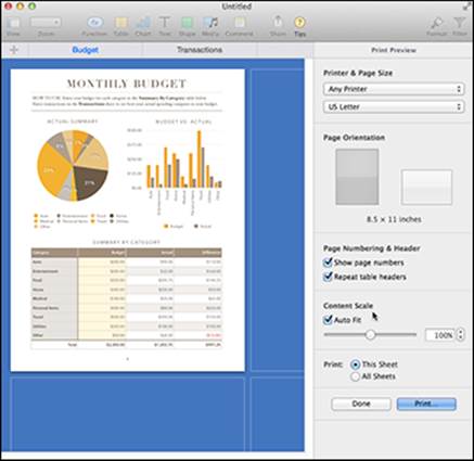
Figure 5-11: Use Print Preview to see how your sheet will print.
3. Drag the Content Scale slider to magnify or shrink your data until it fits exactly the way you want on the page, or select the Auto Fit check box if you want Numbers to do the work for you.
The Content Scale slider is located at the bottom center of the Print Preview pane.
4. Choose any other print options you want and click the Print button.
Exporting a spreadsheet
When you choose File⇒Save, Numbers saves your spreadsheet in its own proprietary file format. If you want to share your spreadsheets with others who don’t have Numbers, export your spreadsheet into another file format by following these steps:
1. Choose File⇒Export to⇒PDF/Excel/CSV/Numbers ’09 on the menu bar.
The Export Your Spreadsheet dialog appears, as shown in Figure 5-12.
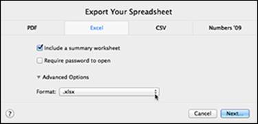
Figure 5-12: Choose a format to save your spreadsheets.
2. Choose one of the following formats:
· PDF: Saves your spreadsheet as a series of static pages stored in the Adobe Acrobat Portable Document Format (PDF) that can be viewed by any computer with a PDF viewing application.
· Excel: Saves your spreadsheet as a Microsoft Excel file, which can be opened and edited by any spreadsheet that can read and edit Microsoft Excel files.
· CSV: Saves your spreadsheet in comma-separated value (CSV) format, which is a universal format that preserves only data, not any charts or pictures you have stored on your spreadsheet.
· Numbers ’09: Saves your spreadsheet as a file that’s compatible with the previous version of Numbers.
The PDF file format preserves formatting 100 percent, but you need extra software to edit it. Generally, if someone needs to edit your spreadsheet and doesn’t use Numbers, choose File⇒Export to⇒Excel. The CSV option is useful only for transferring your data to another application that can’t read Excel files.
The format you choose is highlighted, but you can switch to another one by clicking a different tab.
3. (Optional) If you want to add a password to open the document, select the Require Password to Open check box (all except CSV).
4. Click Next.
A dialog appears, where you choose a name and location to save your exported spreadsheet.
5. Enter a name for your exported spreadsheet in the Save As text box.
6. Click the folder where you want to store your spreadsheet.
You may need to switch drives or folders until you find where you want to save your file. You can also select an external drive or flash drive from the Devices section.
7. Click Export.
 When you export a spreadsheet, your original Numbers spreadsheet remains untouched in its original location.
Sharing files directly from Numbers
You have two more ways to share your spreadsheet:
· Upload the spreadsheet to iCloud.com and then share the link.
When you share the link, anyone who opens it can make changes to it, and those changes will sync to your Mac and iOS devices that access the spreadsheet.
· Share the spreadsheet itself.
Either way, when you share the link or spreadsheet, all the sheets contained in the spreadsheet are included.
Here’s how you can share your presentation via iCloud:
1. Make sure that you saved your presentation on iCloud.
If you aren’t sure how to save your presentation on iCloud, see the “Creating a new spreadsheet with a template” section.
Your presentation must be saved on iCloud for this option to work.
2. Click Share on the toolbar, and then choose Share Link via iCloud.
Choose one of the options:
· Email: Opens a new message with a link to your spreadsheet. Address the message and click Send.
· Messages: Opens a new message with a link to your spreadsheet. Address the message and click Send.
· Twitter: Opens a dialog so you can tweet a link to the spreadsheet. If you aren’t logged in or don’t have a Twitter account, you’re prompted to log in or create an account.
· Facebook: Share the link to your spreadsheet in a status update.
· LinkedIn: Share your spreadsheet with your connections.
· Copy Link: Places the link on the Clipboard so you can paste it somewhere else, such as on your website or in a Keynote presentation.
Here’s how you can send a copy of your spreadsheet to the person who wants to see it:
1. Click Share on the toolbar, and then choose Send a Copy.
This sends a copy of your entire spreadsheet to the destination you choose:
· Messages
· AirDrop
All these choices open a dialog that lets you send the spreadsheet as a Numbers file or as a PDF, an Excel file, or a CSV file.
2. Click the file type and then click Next.
The file is converted if you chose an option other than Numbers.
A new message opens.
3. Type in the address(es) to which you want to send the spreadsheet and then click Send.
For AirDrop, a file is created that other people on your local network with Macs using AirDrop can see and access. See Book III, Chapter 4 to learn more about AirDrop.
After you share a spreadsheet, the Share button on the toolbar changes from an arrow to two bodies.
4. Click the Share button and then View Share Settings to see the link as well as who else is editing it.
Click the Send Link button to share it via Mail, Message, Twitter, Facebook, or LinkedIn.
To remove the link from any place that you’ve shared it, click the Stop Sharing button.
For more tips on using iWork and Numbers, go to Book V, Chapter 6.
All materials on the site are licensed Creative Commons Attribution-Sharealike 3.0 Unported CC BY-SA 3.0 & GNU Free Documentation License (GFDL)
If you are the copyright holder of any material contained on our site and intend to remove it, please contact our site administrator for approval.
© 2016-2026 All site design rights belong to S.Y.A.