iPad All-in-One For Dummies, 7th Edition (2015)

Book IV. Getting Productive with iWork

Chapter 3. Counting on Numbers

In This Chapter

Getting to know Numbers

Working with a template

Using tabs and sheets

Using tables, cells, and forms

Creating new tables

Numbers takes a different approach to the concept of spreadsheets. It brings to spreadsheets not only a different kind of structure but also data formats that you may never have seen. In addition to being able to use numbers and text in your spreadsheets, you can use on-off check boxes and star ratings as part of your data. Think of an inventory spreadsheet with check boxes for in-stock items and star ratings based on reviews or user feedback. What you may have thought of as just a bunch of numbers can now provide true meaning and context to users.

Numbers is a very practical addition to the other iWork apps. Tables and charts are built into both Keynote and Pages, but Numbers is the main number-crunching tool on the iPad.

In this chapter, you discover how Numbers helps organize data into manageable units. After you enter your data, you can display it in charts and graphs.

Introducing Numbers

When you create a Numbers document, you work with these three items:

· A Numbers document: A container for spreadsheets (sheets) and their data; similar to a Microsoft Excel workbook.

· One or more sheets: One or more spreadsheets called simply sheets.

· Tables: The sub-spreadsheets or tables created in other spreadsheet programs exist in Numbers as formal, structured tables rather than as a range of cells within a spreadsheet. Numbers gives them a specific name: tables. (And yes, a Numbers document can have no tables but must have at least one sheet.)

The simple idea of making tables into an actual part of the Numbers application rather than letting people create them any which way leads to a major change in the way you can use Numbers when compared to other spreadsheet programs. Because a table is an entity of its own and not a range of cells, you don’t break the tables you’ve organized in a spreadsheet when you reformat another part of the spreadsheet. You can work within any table, and you can reorganize tables within a sheet, but you can’t break tables by simply adding a row or column to your spreadsheet.

Figure 3-1 shows a Numbers for Mac template (Team Organization).

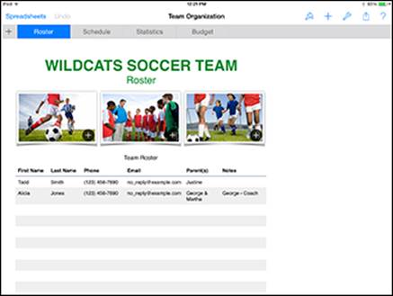
Figure 3-1: The Team Organization template in Numbers for Mac.

Figure 3-1 is a single document with four sheets visible in the tabs in the Sheets pane:

· Roster

· Schedule

· Statistics

· Budget

Some sheets contain tables or charts, and you see them listed in the Sheets pane under their corresponding documents. For example, the Roster sheet contains the Team Roster and Team Management tables (scroll down to see the Team Management table). The Budget sheet contains the Cost Breakdown table as well as a chart (Team Costs). The idea that a single sheet can contain defined charts and tables that don’t depend on ranges of cells is the biggest difference between Numbers and almost every other spreadsheet program.

As you can see in Figure 3-1, sheets can also contain images and other graphics; they aren’t part of the structure of charts and tables. You simply insert these elements the same way you insert any other objects in iWork documents.

You can select individual tables. A selected table has a frame with its column and row titles as well as other controls. Note also that each table within a sheet has its own row and column numbers (you can also name them, if you want) and that each table you deal with starts with cell A1. (The first row is 1 and the first column is A.)

Various tools are available to you in the top-right corner of Numbers, as with other iWork apps. The buttons on this toolbar access settings for formatting tables; for inserting photos, charts, text, and shapes (see Figure 3-2); and for sharing documents and getting help.

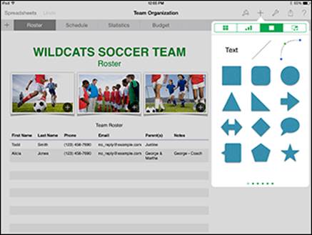
Figure 3-2: The Insert popover in Numbers.

Numbers lets you insert charts along with tables on your sheets, as you see in Figure 3-3. (Remember that you can also insert graphics and other objects on your sheet.)

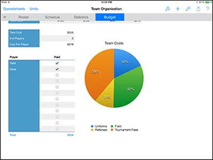
Figure 3-3: You can use charts in Numbers, too.

Numbers also includes the ability to create forms, which simplify data entry. When you create a form, you select a table and you’re taken to a tab that displays each column heading with a text entry box next to it. You can then focus on entering data for one row at a time and eliminate the possibility of accidentally tapping and entering data in the wrong row. You can find more about forms in the “Using Forms Efficiently” section, later in this chapter.

Using the Team Organization Template

This chapter uses the Numbers Team Organization template to demonstrate Numbers features. You can create your own copy of the template so that you can follow along on your iPad, if you want. Sample data is part of the template, so you have data to work with, but you can add any other data you want. After you’ve experimented with Team Organization, you can pick another template, including the Blank template, and customize it for your own data.

To create your own copy of the Team Organization template, follow these steps:

1. Launch Numbers on the iPad.

2. Go to the Documents window.

If you had a spreadsheet open when you were last using Numbers, you return to that spreadsheet. Simply tap Spreadsheets at the top left to go to the Documents window.

3. Tap Create Spreadsheet.

4. Scroll down and tap Team Organization.

Your new spreadsheet opens. Any changes you make are saved automatically.

Working with Tabs and Sheets

Every tab displays a sheet, which can have one or more tables or charts (or both) on it as well as graphics and text frames. Tabs help you organize the contents of your Numbers documents. In this section, I tell you what you need to know about setting up tabs in a document.

Adding a new tab

As with all iWork apps, starting a new Numbers document involves choosing a template. Each template has its own predefined tabs. The Blank template has only one tab (cleverly titled Sheet 1). You can add more tabs by using the plus sign (+) tab on the left end of the tabs (see Figure 3-4).

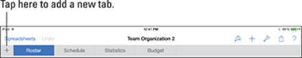
Figure 3-4: The plus sign (+) tab always appears to the left.

Tap the plus sign (+) tab, and Numbers asks whether you want to add a new sheet or a new form. Tap New Sheet, and Numbers creates a new tab that contains one table (see Figure 3-5). The sheet is labeled Sheet 1. See the section “Changing a tab’s name,” later in this chapter, for how to rename the tab. (If you’re interested in forms, I tell you about that topic later in this chapter, in the “Using Forms Efficiently” section.)

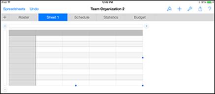
Figure 3-5: Add a new sheet.

Deleting or duplicating a tab

If you add a tab by mistake, you can remove it. Also, if you want to reuse a tab as the basis for a new tab, Numbers allows you to duplicate it. To perform either of these actions, tap and hold the tab you want to delete or duplicate, and a contextual menu appears below it (see Figure 3-6). All you have to do now is tap the option (Duplicate or Delete) for the action you want to take.

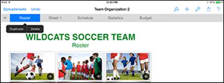
Figure 3-6: Duplicate or delete a tab.

Remember that a double-tap opens the tab so that you can edit its name. A single tap opens the tab’s content. A press-and-hold opens a contextual menu, if available.

Rearranging tabs

If you don’t like the order of your tabs, drag a tab to the right or left in the row of tabs to the desired new position, and then release your finger when the tab is in the position you want (see Figure 3-7).

Figure 3-7: Rearrange tabs.

Navigating tabs

If you have more tabs than can be shown on the screen, just swipe right or left to slide along the tabs. Remember to swipe in the row of tabs. Swiping the body of the sheet scrolls over to the right or left of the content on that sheet.

If you’re holding your iPad in portrait orientation, turn it to landscape orientation to show more tabs on the screen.

Changing a tab’s name

Double-tapping text anywhere in Numbers allows you to edit the text. The same statement applies to tabs, too. Double-tap the name of a tab to begin editing it (see Figure 3-8). The onscreen keyboard appears, and you can delete the current name and enter a new one.

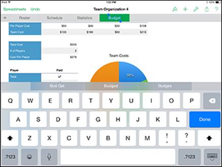
Figure 3-8: Edit a tab’s name.

Using Tables

Tables are at the heart of Numbers — they’re where you enter your data. This section shows you how to work with a table as a whole; the later section “Working with Cells” shows you how to work with individual cells within a table.

Selecting a table

To be able to work on a table, you need to select it. If the table isn’t visible in the current tab, just tap the tab it’s in first. To select a table in Numbers, tap it.

If you need to find an entry within a table, it’s easy to do. Tap the Tools button (the wrench icon near the top-right corner) to open the Tools popover. Tap Find and enter a word or phrase; then tap Search on the keyboard to search the entire Numbers document for a match in that table.

When a table is selected, its appearance changes (see Figure 3-9). A selected table is framed with gray bars above (the column frame) and to its left (the row frame). To the left of the column frame, a button with concentric circles lets you move the table. To the right of the column frame, as well as beneath the row frame, are buttons, each with four small squares (looking a bit like table cells). These Cells buttons let you add rows, columns, or cells and manipulate the cells in the table. (See the later section “Working with Cells.”)

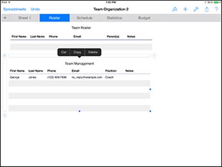
Figure 3-9: Select a table.

Select a table by tapping it once. Note that the location of your tap is important:

· If you tap in a cell, the table and that cell are selected.

· If you tap inside the table bounds but outside the cells, the table itself is selected. For example, if you tap the table’s title or the blank space to the left or right of the title, the table itself is selected. (Refer to Figure 3-9.)

Moving a table

You can move a table around on its sheet. Select the table and tap the round button to the left of the column frame. Then drag the table where you want it. (See Figure 3-10). Numbers shows you the absolute coordinates of the location you’re dragging to. Light-colored lines called guideshelp you align the table to other objects on the sheet. These lines appear and disappear as the table is aligned with the edges or centers of other objects.

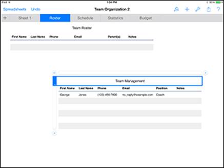
Figure 3-10: Relocate the table.

You can select several objects at the same time. Tap and hold the first object to select it, and then, while still holding down your finger, tap with another finger the other objects you want to add to the selection. After that, they move or resize together. (You may need to use two hands for this task.)

Cutting and pasting a table

You can select a table and then drag it around on a sheet by using the round button at the top left of the column frame; you can resize the table as described in the “Resizing a table” section, later in this chapter. But what if you want to place the table on a different sheet? To copy (or cut) and paste a table onto a different sheet, follow these steps:

1. Select the table by tapping the round button at the top left.

The Cut, Copy, and Delete tools appear, as shown in Figure 3-11.

2. Tap Cut from the selection buttons that appear.

3. Tap the tab of the sheet you want to add the table to.

4. Tap in the sheet (but not in an existing table).

This step brings up new selection buttons.

5. Tap Paste.

6. Move and resize the table as you want.

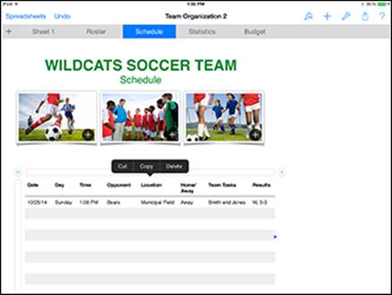
Figure 3-11: Select an entire table.

Adjusting columns or rows

If you’ve ever used a spreadsheet program, you know that data you enter doesn’t always fit into the default column and row sizes. In Numbers, you can select the columns or rows you want to work on and then rearrange or resize them.

Especially with spreadsheets that have lots of rows and columns, resizing can be easier when using a stylus.

Selecting a row or column

Tap in the row frame to select the corresponding row, as shown in Figure 3-12.

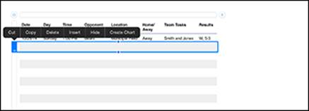
Figure 3-12: Select a row.

Tap in the column frame to select the corresponding column.

After you select a row or column, you can adjust the selection by dragging the handles (the round buttons) at the top and bottom for rows and at the left and right for columns, as shown in Figure 3-13.

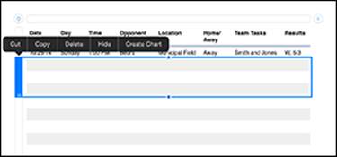
Figure 3-13: Adjust a selection.

The selection buttons Cut, Copy/Paste, Delete, Hide, and Create Chart appear above a selected row, whereas Cut, Copy, Delete, Fill, or Comment appear above a selected cell. Figure 3-14 shows several cells selected within a column.

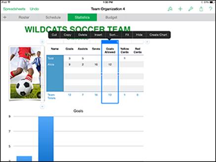
Figure 3-14: Select a few cells in a column.

The selection button you tap affects the selected column or cell.

For example, use the Merge selection button to merge selected cells in a column (or row).

Resizing a row or column

The two vertical lines (known as the Cells button) in the top-right corner of the column frame (refer to Figure 3-14) and the two horizontal lines in the bottom-left corner of the row frame (refer to Figure 3-12) let you resize the selected columns or rows. You always resize a column to its right and a row to its bottom, whether you’re making it larger or smaller. The contents are automatically adjusted, and the adjoining rows or columns are moved aside.

Moving a row or column

Sometimes, you want to rearrange the rows or columns in a sheet. With one or more rows or columns selected, press and drag it (or them) to a new position. All selected rows or columns move as a unit, and the other rows or columns move aside.

Resizing a table

You can resize a table in two ways: add or remove rows or columns to or from the table, or leave the number of rows and columns the same and change the overall size of the table. You may even want to do both.

Adding or removing rows and columns at the right or bottom

Tap the Cells button in the top-right corner of the column frame to add a new column at the right of the table. To add a new row at the bottom, tap the Cells button in the bottom-left corner of the row frame, and a new row is added to the bottom of the table.

To remove a blank column or row at the right side or bottom of a table, drag the appropriate Cells button to the left or to the top of the frame — the extra rows or columns disappear.

Adding or removing rows and columns inside the table

Select the row or column below or to the right of the new row or column. From the selection buttons, tap Insert to add a new row above the selected row or a new column to the left of the selected column.

Changing a table’s size

Select the table so that the handles (small blue dots) are visible at the right side and bottom. These handles work like any other resizing handles in Numbers: Simply drag them horizontally or vertically to change the table’s size. The content of the table automatically resizes to fit the new table size. The numbers of rows and columns remain unchanged, but their sizes may be adjusted.

You can select the table by tapping the round button at the top-left of the table. (Refer to Figure 3-11.)

Read more about formatting tables in the “Working with New Tables” section, later in this chapter.

Working with Cells

Double-tap a cell if you want to add or edit data. A blue outline appears around the cell, and the keyboard appears so that you can begin entering data.

Single-tap if you want to select a cell. The cell is outlined, and the table-selection elements (the column and row frames, the Cells button, the round button to the left of the column frame, and the button to the right of the column frame as well as the button beneath the row frame) appear.

A double-tap makes the cell available for editing. Figure 3-15 shows how, after a double-tap in a cell, the keyboard appears.

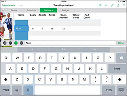
Figure 3-15: Start to edit a cell’s data.

After you set up your spreadsheet, most of your work consists of entering and editing data of all types. That’s what you find out about in the next section.

Entering and editing data

The keyboard for entering data into a Numbers cell is a powerful and flexible tool — it’s four keyboards in one. Above the keyboard, the Formula bar lets you quickly and easily enter formulas. (Refer to Figure 3-15.) On the left of the Formula bar are four buttons that let you switch from one keyboard to another. You can choose these keyboards, starting from the left:

· Numeric (42 icon): Lets you use the numeric keyboard.

· Date and Time (clock icon): Lets you enter dates and times.

· Text (T icon): Displays the standard text keyboard.

· Formulas (= icon): Opens the formula-editing keyboard.

Whichever keyboard you’re using, you see the characters you’re typing in the Formula bar above the keyboard. To the right of the oblong area is a button labeled Done (or a check mark, depending on which keyboard you’re using) that moves your typing into the selected cell and then hides the keyboard.

The Dictation feature on iPad works in Numbers and the other iWork apps. Tap the Dictation key on the onscreen keyboard and speak your text; tap the key again to insert the text in your document.

You can bring up the keyboard when you double-tap a cell or another text field (such as a tab name). That means that the cell is selected and the keyboard knows where the data should go when you tap OK or Done.

Note that many of these features are unavailable on a Bluetooth keyboard, which may or may not have a number pad and special symbols used in entering formulas.

To the right of the keyboard in the numeric and date-and-time keyboards are three large keys:

· Delete: This is the standard keyboard Delete key.

· Next (adjacent): The Next key with the right-pointing arrow inserts the typed data into the selected cell and moves to the next cell to the right.

· Next (next line): The Next key with the hooked arrow pointing left and up inserts the typed data and moves to the next line and to the leftmost cell in the section of cells you’re entering. For example, if you start in the third column of the fourth row, the Next (next line) key moves you to the third column of the fifth row, not the first column.

Entering numeric data

The numeric keyboard (accessed by tapping the 42 button) has a typical numeric keypad along with four large buttons on the left (see Figure 3-16).

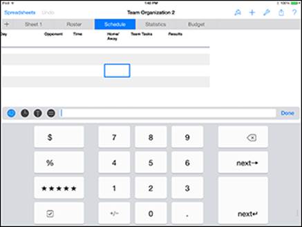
Figure 3-16: Use these tools to input numeric data.

These four buttons let you choose the formatting for the cell you’re editing. If you need a symbol (such as stars for ratings or a currency symbol), it’s added before or after the numeric value as is appropriate. Your formatting options, from top to bottom, are described in this list:

· Currency: This option adds the appropriate currency symbol, such as $, £, or €.

· Percentage: The percent symbol follows the value.

· Stars (rating): This option lets you display a number from 1 to 45 as a star rating. Numbers greater than 5 display with five stars. To change the number of stars, type a new number or tap the star display in the cell or in the display above the keyboard. You can use stars in a spreadsheet and then sort the column of stars so that the ratings are ordered from highest to lowest, or vice versa.

· Check box: A check box is either selected or not. Check boxes are selected and deselected by a user or as the result of a calculation.

Customizing check boxes

A check box can indicate, for example, that an item is in stock or out of stock (yes/no or true/false). However, you can also use it to represent numeric data. Computers and programs often represent nonzero and zero values as yes/no or true/false values. That’s one way you can use check boxes to track inventory. If you show the number of in-stock items in a cell, you can use a check box to indicate that none is in stock (a deselected check box) or that items are in stock (a selected check box). Numbers handles the conversion for you.

Here’s how check box customization can work:

1. Double-tap a cell to start editing it; tap the 42 icon and then tap the Checkbox button when the keyboard opens.

You see a check box in the selected cell; in the area above the keyboard, you see the word false, as shown in Figure 3-17. The green outline distinguishes the word false from text you type in. It has the value false because, before you type anything, its numeric value is zero.

Figure 3-17: A check box starts as off and false.

2. Type a nonzero value.

This value can represent the number of items in stock, for example.

3. Tap the Checkbox button again.

You see that the value you typed changes to true (see Figure 3-18) and that the check box is selected in the table.

Because the formatting is separate from the data value, you can sometimes display the in-stock inventory count as a number and sometimes as the check box. Customers are likely to care only about the check box, but the inventory manager cares about the number.

Figure 3-18: A nonzero value is on and true.

Everything in Numbers is linked, so you don’t have to worry about a sequence for doing most things. If you’ve followed these steps, you’ve seen how to enter a number and have it control a check box, but that’s only one of at least three ways of working with a check box.

With a cell selected and the Checkbox formatting button selected, you see the true/false value above the keyboard and the check box itself in the table cell. Tap the check box in the table cell: The true/false value is reversed, as is the state of the check box itself.

Likewise, if you tap the word true or false in the display above the keyboard, the check box flips its value and true/false reverses.

When you tap a formatting button, it turns blue and formats the number in the selected cell (or cells). You can tap another formatting button to switch to another format (from stars to a percentage, for example). Tapping a highlighted formatting button turns it off without selecting another.

Entering date/time data

Tap the clock button above the keyboard to enter date/time or duration data, as shown in Figure 3-19. The Date & Time button lets you specify a particular moment, and the Duration button lets you specify (or calculate) a length of time.

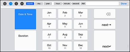
Figure 3-19: Enter date and time, or duration, data.

Above the keyboard, the units of a date or duration display. To enter or edit a date or time (or both), tap Month in the Formula bar and use the keypad to select the month. (The keys have both the month name abbreviations and the month numbers on them.) Similarly, tap any other time increment and enter a value. As you do so, the display changes to show the value. (Tapping AM or PM toggles the value — you don’t need to type anything.)

Entering text data

When you tap the T button to enter text, the standard QWERTY keyboard appears, as shown in Figure 3-20.

As with most onscreen keyboards, you can switch among letters, numbers, and special characters. (If you need a refresher on how to do it, see Book I, Chapter 2.) Everything you type or dictate is inserted into the selected cell until you tap the Done button, which is at the right of the display above the keyboard. If you enter a Return character, it’s part of the text in the cell. The cell automatically expands vertically to accommodate the text you type, and you can resize the column so that the cell is the appropriate size. Remember, these specialized features are not available on Bluetooth keyboards, so it’s often preferable to use the onscreen keyboard when using Numbers.

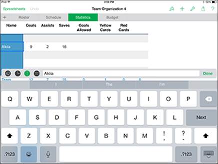
Figure 3-20: Enter text.

Entering formulas

Tapping the equal sign (=) button lets you enter a formula, which automatically computes values based on the data you type. The result of the formula can display in a cell in any of the usual formats, and that value can be used in a chart.

When you’re entering a formula, the four buttons controlling the date-and-time, text, and numeric keyboards disappear. In their place, a button with three dots appears. Tapping this button returns you to the display that gives you access to the other three keyboards. This setup is just a matter of Numbers saving space onscreen.

Formulas are accompanied by good news and bad news. The good news is that you don’t have to type many common formulas: Almost all spreadsheets have the same built-in list of formulas. The bad news is that the list of formulas is quite long.

Formulas can consist of numbers, text, dates, durations, and true/false values. They can also include the results of formulas and the values of individual cells.

The example in this section, which presents the basics of creating a simple formula in Numbers, adds a number to the value of an existing cell and then displays the result in the cell that contains the formula. In this example, I use the Team Organization template that you see in the figures throughout this chapter.

The formula adds 2½ hours to the starting time of a game and displays the estimated completion time in a new column. Follow these steps:

1. Rename the Time column in the Schedule tab to Start.

2. Add a column to its right and name it End.

3. Select the cell in which you want to insert the formula by double-tapping it.

I selected the End column cell next to Start, as you can see in Figure 3-21.

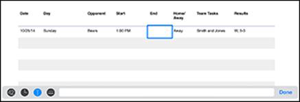
Figure 3-21: Select the cell that will contain the formula.

4. Tap the equal sign (=) button at the top-left side of the keyboard.

The keyboard changes to the formula keyboard, as shown in Figure 3-22.

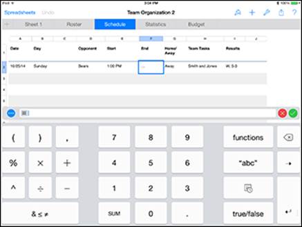
Figure 3-22: Begin to create a formula.

The table’s column and row frames now contain row and column identifiers. The columns are labeled A, B, C, and so on; the rows are labeled 1, 2, 3, and so on. Every cell can be identified by its coordinates (such as A1 for the top-left cell).

Also note that at the right of the keyboard is a different set of buttons than on the text, date, and number keyboards. On the right side of the keypad, you’ll find four buttons that represent the following:

· Functions: Brings up a list of functions for use in formulas. (Refer to Step 3.)

· abc: Displays the text keyboard. You can type text and tap Done, and the text is added to the formula you’re constructing. You return to the formula keyboard.

· Date/Time: Takes you to the date-and-time keyboard. The date or duration you enter uses the same interface shown in Figure 3-19. When you tap Done, the date or duration is added to the formula, and you return to the formula keyboard.

· True/False: Uses the same interface as check boxes; the result is added to the formula you’re constructing, and you return to the formula keyboard.

5. Add the game starting time to the formula.

Just tap the cell containing the game start time. The formula reflects the name of the table and the referenced cell. In this case, that reference is

C2

This references column C, row 2 in the Game Schedule table. You don’t have to type a thing — just tap, and the correct cell is referenced.

You now need the formula to add 2½ hours to the starting time.

6. Tap + from the operators on the left side of the keyboard.

7. Tap the Date/Time button on the right side of the keyboard and then tap the Duration button at the left.

8. On the Formula bar, tap Hours and enter 2.

9. Tap Minutes and enter 30.

Figure 3-23 shows what the screen looks like now.

10. Tap Done.

You’re done entering the duration. You return to the formula keyboard.

11. Finish the formula by tapping the button with a check mark on it.

Figure 3-24 shows the formula as it is now. Note that rather than seeing the Done button, as with other keyboards, you see a button with a check mark and a button with an X at the right. The X cancels the formula, and the check mark completes it. If you want to modify the formula with the keys (including Delete) on the keyboard, feel free.

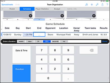
Figure 3-23: Enter the formula.

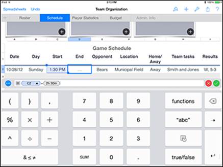
Figure 3-24: Tap the check mark to accept the formula.

Changing a cell’s content formatting

Your end time may include the date, which is probably not what you want. Here’s how to change the formatting of a cell’s contents:

1. Select the cell by making a single tap.

You can also select a cell and drag the highlighted selection to include more than one cell. Your reformatting affects all selected cells.

2. Tap the Format button at the top of the screen.

3. In the Format popover, tap the Information button to the right of Date & Time.

4. Tap the format you want to use in the selected cell or cells, or tap the arrow at the right of the format name to customize the format.

Not all formats have customizations.

To properly format the end time cell, you may want to remove the date. In the Date & Time Options popover, set the date option for None, as shown in Figure 3-25, and the time option for the hour.

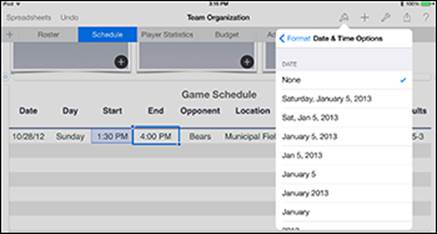
Figure 3-25: Format the result.

Using Forms Efficiently

A form is a user-friendly way to provide input to a single row of a spreadsheet. Because a form interacts with a table, you must create a table in your spreadsheet before you can create an associated form.

To create a form, tap the plus sign (+) tab on the left end of the row of tabs. You’re asked whether you want to create a new sheet or a form. (Refer to Figure 3-25.) Tap New Form, and you see a screen similar to the one shown in Figure 3-26, which uses the Team Organization template for the example.

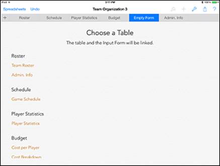
Figure 3-26: Start to create a form.

You see a list of all the sheets and all the tables on them. Choose the one that the form will be used with. In this case, I’m using my Team Management table.

Every form is associated with only one table, and every table can be associated with only one form (though it doesn’t have to be associated with any forms).

The form is then created automatically, as shown in Figure 3-27.

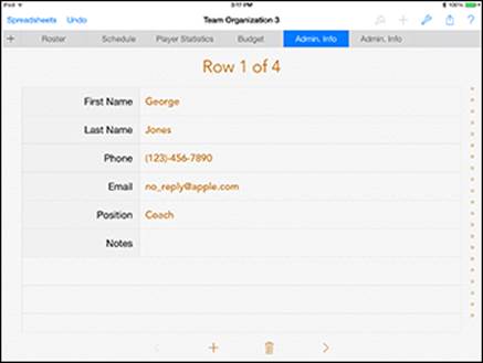
Figure 3-27: Use a form to browse, enter, and delete data.

The labels for the rows on the form are drawn from the labels of the columns on the tables. You don’t have to label the columns on your tables, but it makes creating forms and calculations much easier if you do.

You can use the tab to go to the form and enter data or browse it. The four buttons at the bottom of a form let you (from left to right) go to the previous record (row), add a new row, delete the current row, or go to the next row.

You can delete a form by tapping the form’s tab and then tapping Delete, but you can’t duplicate a form as you can duplicate a sheet tab.

Working with New Tables

Tables contain the data for your spreadsheets and charts, so it may be a bit surprising if you’ve reached the end of the chapter without creating a single table. That’s because you have numerous templates to work with. You don’t have to start from the beginning; instead, you can start from further along in the development process.

Tables can be relatively small and focused. You can use formulas to link them, and that’s a much better strategy than putting every single piece of data into an enormous spreadsheet.

Tables aren’t simply repositories of data; they also drive charts. When you’re organizing data in a table, you may want to consider how to transform it to create the kind of charts you want.

As you’re planning the structure of your tables and sheets, pay attention to the moments when you realize that you have to add more data to a table. Ask whether you truly need more data in that table or need a table that can be linked to the first table by a calculation.

A table often has a header row above its data rows; the header row usually contains titles but may also contain calculations such as sums or averages. Numbers tables can have several header rows. A column to the left of the table also has the same functionality — it’s a header column. People often believe that a header appears only at the top, but in this usage, it appears on whichever side is appropriate.

Creating a new table

Follow these basic steps to create a new table:

1. Go to the sheet you want the table to be on.

It can be an existing sheet from a template or a new sheet you create just for the table. Remember that tables can be cut and pasted, so you have a second (and third and fourth and so on) chance to determine the sheet for your table.

2. Tap the Insert Objects button (the + button) in the toolbar at the top of the window.

The Insert Objects popover opens.

3. Tap the Tables tab.

4. Swipe from one page to another to find the table layout you like.

Though you can change any element in the table layout, start with one close to what you want to end up with.

There are five pages of templates — each of the five pages has the same layouts but with different color schemes. This list describes them from the upper-left corner, as shown in Figure 3-28:

· Header row and a header column at the left: This is one of the most common table layouts.

· Header row at the top: This one works well for a list such as students in a class.

· No header row or header column: Before choosing this blank spreadsheet, reconsider. Headers and titles for the tables make your spreadsheet more usable. You can add (or delete) them later and change them, but take a few moments to identify the table along with its rows and columns as soon as you create it.

· Header and footer rows and a label column: This one works well for titles at the top and left and for sums or other calculations at the bottom.

· Check boxes in the left column: This option makes a great list of things to do.

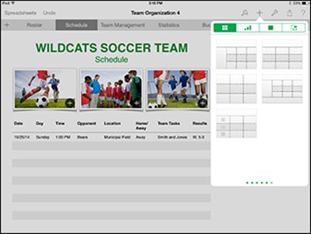
Figure 3-28: Create a new table.

5. Tap the table layout you like.

It’s placed on the sheet you have open.

Changing a table’s look

Whether you recently created a new table or created it long ago, you might want to change its appearance. Here’s how:

1. Select the table you want to format (to select the table, tap inside the table bounds but outside the cells) and tap the Format button in the toolbar.

The Format popover opens, as shown in Figure 3-29. You can change the basic color scheme and layout by tapping the design you want to use.

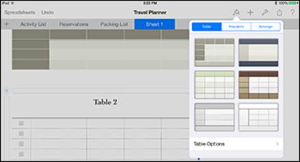
Figure 3-29: Use Format to reformat a table.

2. Tap Table Options and fine-tune the table with a title, outline, and shading for alternating rows (see Figure 3-30).

Every table has a name. (It starts as Table #, with the next sequence number for all your tables.) The Table option simply controls whether the title is shown. Change the name to something meaningful that you can use in referencing it in formulas. Likewise, each table is a certain size. The Table Outline option determines whether a thin line is applied as the table’s border. In the Alternating Rows option, every other row is shaded with a contrasting color.

For large tables, alternating the shading of the rows can make it easier for users to follow the data.

3. Tap Grid Options to show or hide the cell dividers.

Many people think that showing the lines in the main table and hiding them in the headers looks best. Experiment. As you tap to turn options on or off, the display changes so that you can see the effect.

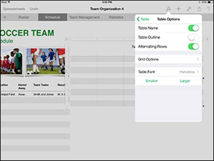
Figure 3-30: Set table options.

4. Tap Table Options to return to that popover and then tap Table Font or the Smaller or Larger text size buttons to format the text in the table.

5. Tap Table in the popover and then tap the Headers tab to modify headers for rows and columns.

You can set the number of header rows or columns. (You have either zero footer rows or one footer row.) These elements are created using the existing color scheme.

Freezing rows and columns keeps the header rows and columns on each page. As you scroll the data, the data itself moves, but the headers never scroll out of sight. This option is often the best one unless the table’s content is self-explanatory.

6. When you’re finished, tap anywhere outside the popover to close it.