Pro Office for iPad: How to Be Productive with Office for iPad (2014)
Chapter 9. Using Formulas and Functions in Your Worksheets
Many of your worksheets will likely need to perform calculations with your data. To perform calculations in Excel, you enter formulas and functions in the appropriate cells in the worksheets. This chapter will explain what formulas and functions are, and what the difference between them is, and then shows you how to use each. Along the way, you will learn how to refer to cells and ranges, meet the calculation operators that Excel supports, and discover how to use them. You will also learn about common problems that occur with formulas and ways to troubleshoot them.
Understanding the Difference Between Formulas and Functions
In Excel, you can perform calculations in two main ways, each of which starts with an equal sign:
· By using a function: A function is a preset formula that performs a standard calculation. For example, when you need to add several values together, you use the SUM() function; for instance, =SUM(1,2,3,4,5,6) is simpler than =1+2+3+4+5+6 but has the same effect.
· By using a formula: A formula is a custom calculation that you create when none of Excel’s functions does what you need. At its simplest, a formula can be a straightforward calculation; for example, to subtract 50 from 100, you can type =100-50 in a cell (the equal sign tells Excel you’re starting a formula). Formulas can also be more complex, as you’ll see in due course.
You can use functions as needed in your formulas. For example, say you need to add the contents of the cells in the range A1:A6 and then divide them by the contents of cell B1. Excel doesn’t have a built-in function for doing this because it’s not a standard calculation. So instead, you create a formula such as this: =SUM(A1:A6)/B1. (In this example, the / is the keyboard equivalent of the ÷ symbol.)
You will learn how to use both functions and formulas. I’ll start with formulas, but first, let’s go over the ways of referring to cells and ranges in formulas and functions.
Referring to Cells and Ranges in Formulas and Functions
To make your formulas and functions work correctly, you need to refer to the cells and ranges you want. This section makes sure you know how to refer to cells and ranges, both when they’re on the same worksheet as the formula and when they’re on a different worksheet.
Referring to a Cell
To refer to a cell on the same worksheet, simply use its column lettering and its row number. For example, use =A10 to refer to cell A10.
To refer to a cell on a different worksheet, enter the worksheet’s name followed by an exclamation point and the cell reference. For example, use =Supplies!A10 to refer to cell A10 on the worksheet named Supplies. The easiest way to set up such a reference is via these steps.
1. Double-tap the cell in which you want to enter the formula. Excel displays the Formula bar and the keyboard.
2. If the letters keyboard is displayed, tap the 123 button in the upper-right corner of the keyboard to display the numbers keyboard. (Tapping the .?123 button gives you the regular numbers keyboard, which is less useful in Excel because it is not optimized for entering data and formulas).
3. Tap the = key. Excel automatically displays the Functions pop-up panel (see Figure 9-1).
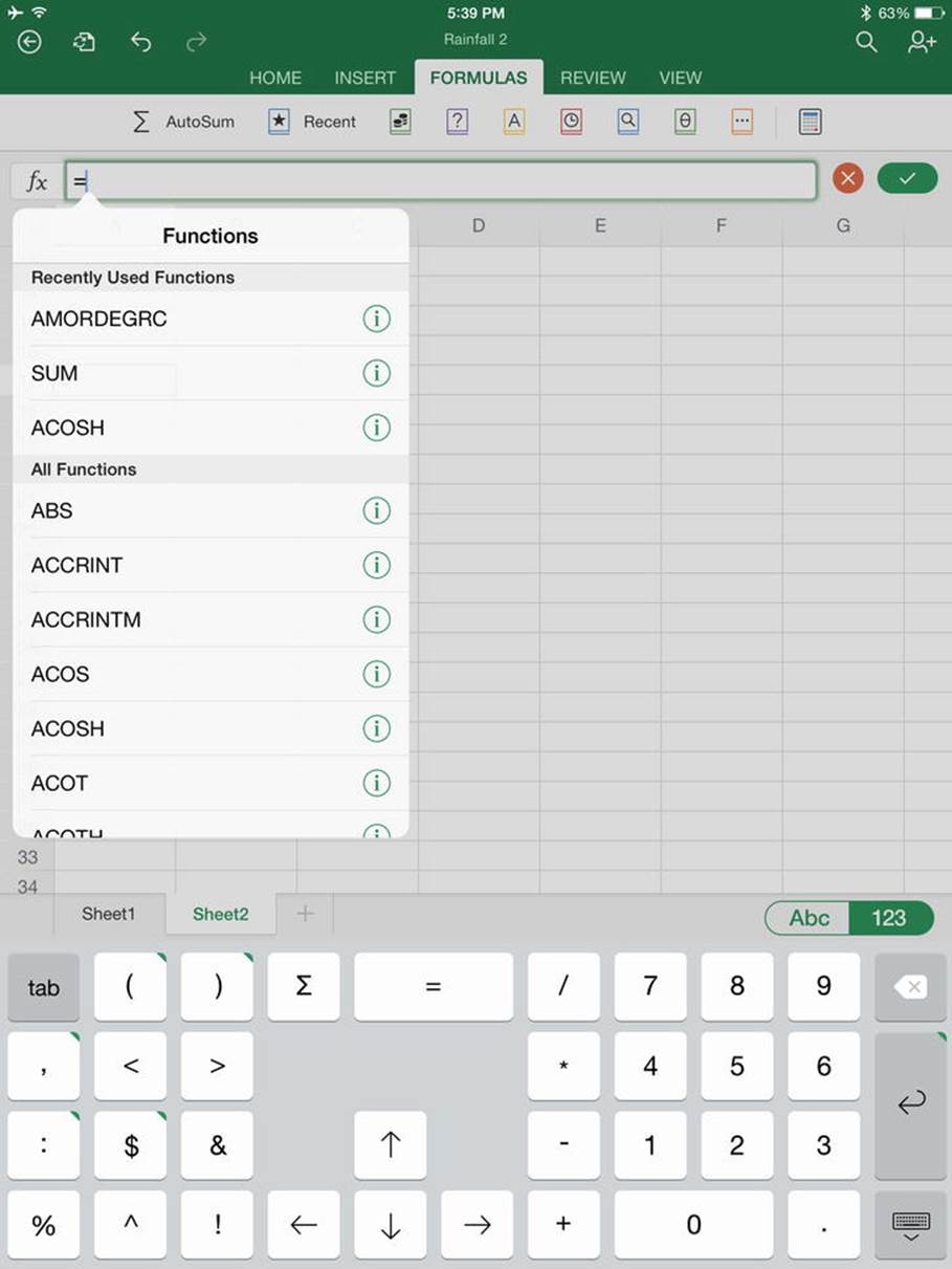
Figure 9-1. Excel automatically displays the Functions pop-up panel when you double-tap a cell and type an equal sign
4. Tap anywhere in the spreadsheet to close the Functions pop-up panel.
5. Tap the worksheet tab for the worksheet that contains the cell you want to refer to.
6. Tap the cell.
7. Tap the Enter button, the green button with the white check mark at the right end of the Formula bar, to enter the reference. Excel returns you to the worksheet on which you’re creating the formula.
8. Double-tap the cell to resume editing its contents.
9. Finish creating the formula, and then tap the Enter button. You can also tap the Return key on the keyboard.
Note Tapping the Return key on the keyboard enters the formula in the cell and moves the active cell down by one cell. If necessary, you can double-tap the previous cell to edit its contents.
Instead of using the method just described to enter a reference to another worksheet, you can type in the worksheet’s name and the reference. There’s one complication: if the worksheet’s name contains any spaces, you must put the name inside single quotes, for example, =‘Sales Results’!A10 rather than =Sales Results!A10. You can also use the single quotes on worksheet names that don’t have spaces if you find it easier to be consistent. If you omit the single quotes when they’re needed, Excel displays an error message.
Note If you refer to a named cell in a formula, the formula displays that name, not the reference.
CREATING A FORMULA USING A HARDWARE KEYBOARD
If you’re using a hardware keyboard with your iPad, you can enter a formula using different techniques from using the touchscreen:
· Tap the target cell instead of double-tapping it. When using a hardware keyboard, you don’t need to open the cell for editing; simply select the cell and then type =.
· Alternatively, use the arrow keys to move the active cell to the target cell. You can also press the Tab key to move the active cell to the right by one cell or press the Enter key to move the active cell down by one cell.
· Press the Enter key to enter the formula in the cell instead of tapping the Enter button on the Formula bar.
DEALING WITH EXTERNAL REFERENCES IN WORKBOOKS
The desktop versions of Excel enable you to create external references, references to cells and ranges in other workbooks. This type of reference also has a strict format: first the workbook’s path, then the file name in brackets, then the worksheet’s name, and then the cell reference. For example, the reference ='Common:Spreadsheets:[Results.xlsx]Sales!'AB12 refers to cell AB12 on the worksheet named Sales in the workbook Results.xlsx in the Common:Spreadsheets folder on a Mac.
Excel for iPad cannot handle external references at this writing. When you open a workbook that contains an external reference, Excel displays the Cannot Update Workbook dialog box to warn you of the problem. When you dismiss this dialog box, Excel lets you work in the workbook, but it’s best not to continue, for two reasons. First, the data may not be current, so your calculations may contain unknown horrors; and second, changes you make to the workbook may break references, which can cause you trouble when you next open the workbook on your PC or Mac.
Excel for iPad allows you to create external links in your workbooks, but because the data is not available, Excel displays the value 0 (zero) for those links. It is best not to create external links on Excel for iPad because you can’t see the results until you open the workbook in a desktop version of Excel.
Referring to a Range
To refer to a range that consists of a block of cells, enter the addresses of the first cell and the last cell, separating them with a colon. For example, to refer to the range from cell P10 to cell Q12, use =P10:Q12. You can enter the range address in several ways:
· Type in the range address, including the colon.
· Tap the first cell in the range, type the colon, and then tap the last cell.
· Tap the first cell in the range and drag through to the last cell.
To refer to a range that consists of individual cells, give the address of each cell, separating the addresses with commas. For example, to add the values in cell J14, cell K18, and cell Z20, use =SUM(J14,K18,Z20).
To refer to a range on a different worksheet, use the technique explained in the previous section. For example, if you need to work out the average value of the values in the range P10 to P22 on the worksheet named Stock Listing, use =AVERAGE('Stock Listing'!P10:P22).
Making One Row or Column Refer to Another Row or Column
Sometimes you may need to make the contents of one row or column refer to another row or column. For example, say you need to make each cell in column J refer to the corresponding cell in column C, so that cell J1 refers to cell C1, cell J2 to cell C2, and so on.
To do this, follow these steps.
1. Tap the first cell in the column in which you want to enter the data—in this case, cell J1.
2. Tap in the Formula bar to display the keyboard.
3. Tap the = button to start creating the formula. The Functions pop-up panel appears.
4. If the Functions pop-up panel is in the way, tap anywhere in the worksheet to close it.
5. Tap the column heading for column C to make Excel enter the formula =C:C.
6. Tap the Enter button at the right end of the Formula bar to enter the formula.
7. Use AutoFill to copy the formula to the other cells in column J.
Similarly, you can refer to a whole row by entering its letter designation, a colon, and the letter designation again; for example, 2:2.
Understanding Absolute References, Relative References, and Mixed References
Using cell addresses or range addresses is straightforward enough, but when you start using formulas, there’s a complication. When you copy a formula and paste it in a different location, you need to tell Excel whether the pasted formula should refer to the cells it originally referred to, or the cells in the same relative positions to the cell where the formula now is, or a mixture of the two. (If you move a formula to another cell by using drag and drop or cut and paste, Excel keeps the formula as it is.)
To make clear exactly what each reference refers to, Excel uses three types of references:
· Absolute reference: A reference that always refers to the same cell, no matter where you copy it. Excel uses a dollar sign ($) to indicate that each part of the reference is absolute. For example, $B$3 is an absolute reference to cell B3.
· Relative reference: A reference that refers to the cell by its position relative to the cell that holds the reference. For example, if you select cell A3 and enter =B5 in it, the reference means “the cell one column to the right and two rows down.” So if you copy the formula to cell C4, Excel changes the cell reference to cell D6, which is one column to the right and two rows down from cell C4. To indicate a relative reference, Excel uses a plain reference without any dollar signs, such as B5.
· Mixed reference: A reference that is absolute for either the column or the row and relative for the other. For example, $B4 is absolute for the column (B) and relative for the row (4), while B$4 is relative for the column and absolute for the row. When you copy and paste a mixed reference, the absolute part stays the same, but the relative part changes to reflect the new location.
If you’re typing a reference, you can type the $ sign into the reference to make it absolute or mixed. If you’re entering references by selecting cells, follow these steps to change the reference type.
1. Tap the cell to which you want to refer, or tap and drag to select a range. The reference appears in the Formula bar.
2. Tap the reference in the Formula bar to select it. The reference changes color.
3. Tap the selected reference to display the Edit menu.
4. Tap the Reference types button to display the Cell Reference Types pop-up panel.
5. Tap the reference you want: Relative Column, Relative Row; Absolute Column, Absolute Row; Relative Column, Absolute Row; or Absolute Column, Relative Row.
Note If a formula refers to multiple cells, you need to alter the reference for each cell separately. There’s no mechanism for altering each reference to the same type in a single move.
Referring to Named Cells and Ranges
If your workbook contains named cells or ranges, you can refer to them easily in formulas by entering their names. For example, if you have named one cell Income and another cell Expenditure, you can use a formula such as =Income – Expenditure to calculate the net remaining.
Tip Names for cells and ranges must be unique within a workbook, so you don’t need to specify the worksheet when referring to a named cell or range.
At this writing, Excel for iPad cannot create named cells or ranges, so you need to create them in a desktop version of Excel instead.
Creating Formulas to Perform Custom Calculations
When you need to perform a custom calculation in a cell, you create a formula that tells Excel what you want to do. The formula uses the appropriate calculation operators, such as + signs for addition and – signs for subtraction. In this section, you will meet the calculation operators, try using them in a worksheet, and learn the order in which Excel applies them and how to change that order.
Understanding Excel’s Calculation Operators
To perform calculations in Excel, you need to know the operators for the different operations—addition, division, comparison, reference, and text. Table 9-1 explains the full set of calculation operators you can use in your formulas in Excel.
Table 9-1. Excel’s Calculation Operators
|
Calculation Operator |
Operation |
Explanation or Example |
|
Arithmetic Operators |
||
|
+ |
Addition |
=1+2 adds 2 to 1. |
|
– |
Subtraction |
=1–2 subtracts 2 from 1. |
|
* |
Multiplication |
=2*2 multiplies 2 by 2. |
|
/ |
Division |
=A1/4 divides the value in cell A1 by 4. |
|
% |
Percentage |
=B1% returns the value in cell B2 expressed as a percentage. Excel displays the value as a decimal unless you format the cell with the Percentage style. |
|
^ |
Exponentiation |
=B1^2 raises the value in cell B1 to the power 2. |
|
Comparison Operators |
||
|
= |
Equal to |
=B2=15000 returns TRUE if cell B2 contains the value 15000. Otherwise, it returns FALSE. |
|
<> |
Not equal to |
=B2<>15000 returns TRUE if cell B2 does not contain the value 15000. Otherwise, it returns FALSE. |
|
> |
Greater than |
=B2>15000 returns TRUE if cell B2 contains a value greater than 15000. Otherwise, it returns FALSE. |
|
>= |
Greater than or equal to |
=B2>=15000 returns TRUE if cell B2 contains a value greater than or equal to 15000. Otherwise, it returns FALSE. |
|
< |
Less than |
=B2<15000 returns TRUE if cell B2 contains a value less than 15000. Otherwise, it returns FALSE. |
|
<= |
Less than or equal to |
=B2<=15000 returns TRUE if cell B2 contains a value less than or equal to 15000. Otherwise, it returns FALSE. |
|
Reference Operators |
||
|
[cell reference]:[cell reference] |
The range of cells between the two cell references |
A1:G5 returns the range of cells whose upper-left cell is cell A1 and whose lower-right cell is cell G5. |
|
[cell reference],[cell reference] |
The range of cells listed |
A1,C3,E5 returns three cells: A1, C3, and E5. |
|
[cell or range reference] [space][cell or range reference] |
The range (or cell) that appears in both cells or ranges given |
=A7:G10 B10:B12 returns the cell B10, because this is the only cell that appears in both the ranges given. If more than one cell appears in the range, this returns a #VALUE! error. |
|
Text Operator |
||
|
& |
Concatenation (joining values as text) |
=A1&B1 returns the values from cells A1 and B1 joined together as a text string. For example, if A1 contains “South America ” (including a trailing space) and B1 contains “Sales”, this formula returns “South America Sales.” If A1 contains 100 and B1 contains 50, this formula returns 10050. |
Using the Calculation Operators
Now that you know what the calculation operators are, try the following example of creating a worksheet (see Figure 9-2) with formulas that use the four most straightforward operators—addition, subtraction, multiplication, and division.
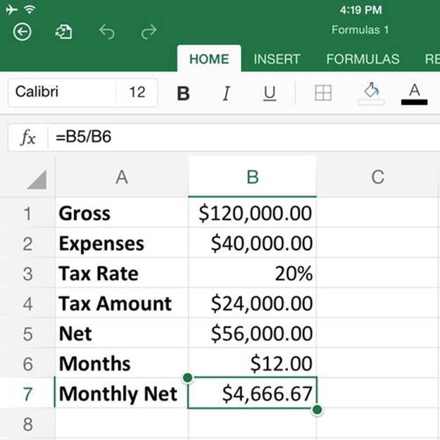
Figure 9-2. Create this worksheet to try using Excel’s addition, subtraction, multiplication, and division operators
To create the worksheet, follow these steps.
1. Create a new workbook.
a. If you’re currently in a workbook, tap the Back button.
b. Tap the New tab in the tab bar to display the New screen.
c. Tap the New Blank Workbook icon.
2. Type the following text in cells A1 through A7:
o A1: Gross
o A2: Expenses
o A3: Tax Rate
o A4: Tax Amount
o A5: Net
o A6: Months
o A7: Monthly Net
3. Apply boldface to column A.
. Tap the column heading to select the column.
a. Tap the Home tab of the Ribbon to display its controls.
b. Tap the Bold button.
4. Apply the Currency format to column B.
. Tap the column heading to select the column.
a. Tap the Number Formatting pop-up button to display the Number Formatting pop-up panel.
b. Tap the Currency button.
5. Type the following text in cells B1 through B3:
o B1: 120000
o B2: 40000
o B3: 0.2
6. Apply the Percent style to cell B3.
. Tap cell B3.
a. Tap the Number Formatting pop-up button to display the Number Formatting pop-up panel.
b. Tap the Percentage button. The readout changes from $0.20 to 20%.
7. Now enter the formula =B1*B3 in cell B4, like this:
. Double-tap cell B4 to select it, open it for editing, and display the keyboard.
a. Type = to start creating a formula in the cell. The Functions pop-up panel appears.
b. Tap anywhere in the worksheet to close the Functions pop-up panel.
c. Tap cell B1 to enter it in the formula. Excel displays a shimmering dotted blue outline around the cell and adds it to the formula in the cell and to the Formula bar (see Figure 9-3).
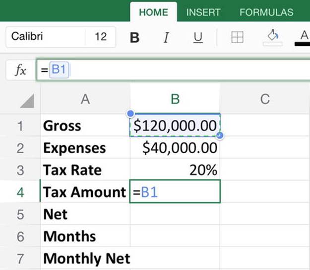
Figure 9-3. When you tap cell B1, Excel adds it to the formula in both the cell and the Formula bar and displays a dotted blue outline around it
d. Type * to tell Excel you want to multiply the value in cell B1. Excel enters the asterisk in the formula and changes the outline around cell B1 to solid blue.
e. Tap cell B3 to enter it in the formula. Excel displays a shimmering dotted outline (red this time) around the cell and adds it to the formula in the cell and in the formula bar (see Figure 9-4).
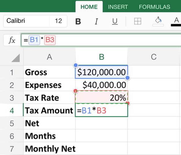
Figure 9-4. Tap cell B3 to add it to the formula
f. Tap the Enter button (the green button with the check mark at the right end of the Formula bar) to finish entering the formula in cell B4.
8. Enter the formula =B1-(B2+B4) in cell B5. Follow these steps.
. Double-tap cell B5 to select it, open it for editing, and display the keyboard.
a. Type = to start creating a formula in the cell. The Functions pop-up panel appears.
b. Tap anywhere in the worksheet to close the Functions pop-up panel.
c. Tap cell B1 to add it to the formula.
d. Type – to enter the subtraction operator.
e. Type ( to start a nested expression. (You’ll learn about nesting shortly.)
f. Tap cell B2 to add it to the formula.
g. Type + to enter the addition operator.
h. Tap cell B4 to add it to the formula.
i. Type ) to end the nested expression.
j. Tap the Enter button to finish entering the formula.
9. Enter 12 in cell B6 and apply General formatting to it. Follow these steps.
. Tap cell B6 to select it.
a. Tap the Number Formatting pop-up button to display the Number Formatting pop-up panel.
b. Tap the General button.
c. Double-tap cell B6 to select it, open it for editing, and display the keyboard. The Functions pop-up panel opens.
d. Tap anywhere in the worksheet to close the Functions pop-up panel.
e. Type 12.
f. Tap the Enter button on the keyboard to enter the value and move the active cell to cell B7.
10.Enter the formula =B5/B6 in cell B7. This time, simply type the formula in—lowercase is fine—and then tap Return. You’ll notice that when you type each cell reference, Excel selects that cell to let you check visually that you have the right cell.
11.Tap the Enter button to enter the formula in the cell. You’re done.
Now that you’ve created the worksheet, try changing the figures in cells B1, B2, and B3. You’ll see the results of the formulas in cells B4, B5, and B7 change accordingly. Excel recalculates the formulas each time you change a value in a cell, so the formula results remain up to date.
Note The desktop versions of Excel enable you to turn off automatic recalculation and force recalculation manually. Turning off automatic recalculation is useful for large workbooks containing many calculated values, especially when one recalculated value causes many other values to need recalculation. Excel for iPad does not let you turn automatic recalculation on or off at this writing. But if you open a workbook that has automatic recalculation turned off, you can recalculate it manually: tap the Formulas tab to display its controls, and then tap the Recalculate button, the button on the far right that shows a calculator icon.
Overriding the Order in Which Excel Evaluates Operators
When you need to use multiple operators in a formula, you must understand the order in which Excel evaluates the operators so that you can get the calculation correct. You can also override the default evaluation order to make your formulas work the way you intend.
In the previous example, you entered the formula =B1-(B2+B4) in cell B5. The parentheses are necessary because the calculation has two separate stages—one stage of subtraction and one stage of addition—and you need to control the order in which they occur.
Try changing the formula in cell B5 to =B1-B2+B4 and see what happens. Follow these steps.
1. Double-tap cell B5 to open it for editing.
2. Tap in the Formula bar to start editing the formula there.
3. Delete the opening and closing parentheses.
4. Tap the Enter button at the right end of the Formula bar.
You’ll notice that the Net amount (cell B5) jumps substantially. This is because you’ve changed the meaning of the formula.
· =B1-(B2+B4). This formula means “add the value in cell B2 to the value in cell B4, and then subtract the result from the value in cell B1.”
· =B1-B2+B4. This formula means “subtract the value in cell B2 from the value in cell B1, and then add the value in cell B4 to the result.”
Double-tap cell B5 to open the cell for editing. Position the insertion point before B2 and type (; then position the insertion point after B4 and type ). Then tap the Enter button to enter the formula in the cell.
The order in which Excel evaluates the operators is called operator precedence, and it can make a huge difference in your formulas, so it’s vital to know both how it works and how to override it. Table 9-2 shows you the order in which Excel evaluates the operators in formulas.
Table 9-2. Excel’s Operator Precedence in Descending Order
|
Precedence |
Operators |
Explanation |
|
1 |
– |
Negation |
|
2 |
% |
Percentage |
|
3 |
^ |
Exponentiation |
|
4 |
* and / |
Multiplication and division |
|
5 |
+ and – |
Addition and subtraction |
|
6 |
& |
Concatenation |
|
7 |
=, <>, <, <=, >, and >= |
Comparison operators |
When two operators are at the same level, Excel performs the operator that appears earlier in the formula first.
Nesting Parts of a Formula to Control Operator Precedence
You can control operator precedence in any formula by nesting one or more parts of the formula in parentheses. For example, as you just saw, using =B1-(B2+B4) makes Excel evaluate B2+B4 before the subtraction.
You can nest parts of the formula several levels deep if necessary. For example, the following formula uses three levels of nesting and returns 180:
=10*(5*(4/(1+1))+8)
Note If you’ve ever worked out math equations by hand, you know how you start by calculating the innermost (most deeply nested) set of parentheses and then work outward, applying the order of operator precedence within each level of nesting. Excel works in just the same way, following common mathematical rules.
Breaking Up a Complex Formula into Separate Steps
Excel enables you to create a highly complex formula in a single cell. If you like math, science, or logic, you may enjoy creating such formulas. It’s certainly satisfying when they work, but they can be hard to troubleshoot when they don’t.
To make troubleshooting (or simply changing) your formulas easier, consider breaking up any complex formula into separate steps, putting each step in its own cell or row. For example, you could break up that =10*(5*(4/(1+1))+8) formula like this:
· Cell B1. =1+1
· Cell B2. =4/B1
· Cell B3. =5*B2
· Cell B4. =B3+8
· Cell B5. =10*B4
Broken up like this, each formula is easy to read, and you can easily see if any of the steps gives the wrong result. You can type a text description of each step in the next cell for reference, or (more discreetly) insert a comment describing the step.
When you’ve checked that the formula works, you have the option of creating a new version of the formula that goes into a single cell. But if you want to keep the worksheet easy to read and easy to audit, leave the formula in its step-by-step form.
Entering Formulas Quickly Using Copying and AutoFill
In many worksheets, you’ll need to enter related formulas in several cells. For example, say you have the worksheet shown in Figure 9-5, which lists a range of products with their prices and sales. Column D needs to show the total revenue derived by multiplying the Units figure by the Price value.
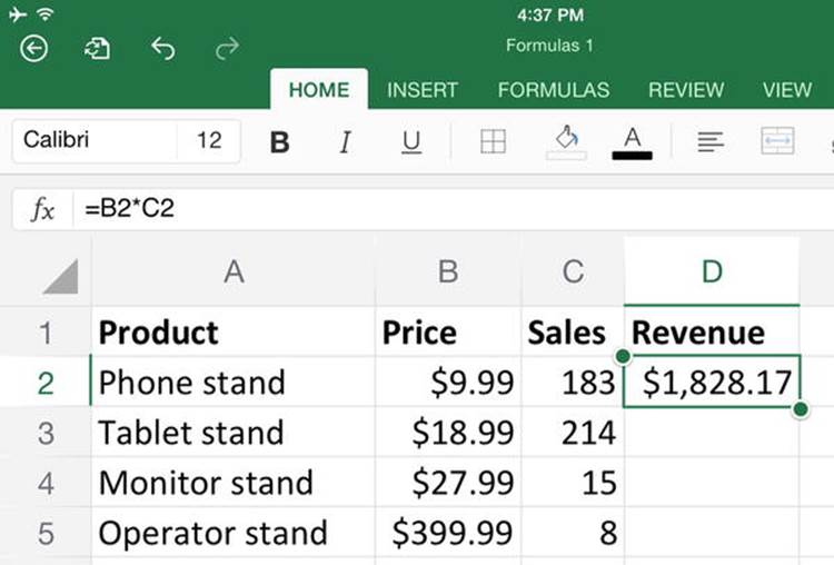
Figure 9-5. When a worksheet needs similar formulas in a column or row, you can enter one formula manually and then use the AutoFill or Copy and Paste features to enter it quickly in the other cells
Each cell in column D needs a different formula: Cell D2 needs =B2*C2, Cell D3 needs =B3*C3, and so on. Because the formula is the same except for the row number, you can use either AutoFill or Copy and Paste to enter the formula from cell D2 into the other cells as well.
To enter the formula using AutoFill, follow these steps.
1. Tap the cell that contains the formula—in this case, cell D2.
2. Tap the cell again to display the Edit menu.
3. Tap the Fill button to display the AutoFill handles.
4. Drag the appropriate handle (in this case, the downward handle) down through cell D5. Excel automatically fills in the formulas, adjusting each for the change in row.
To enter the formula using Copy and Paste, use the Copy and Paste commands.
1. Tap the cell that contains the formula.
2. Tap the cell again to display the Edit menu.
3. Tap the Copy command.
4. Tap to select the first cell in the destination range.
5. Drag a selection handle to select the rest of the destination range. The Edit menu appears automatically.
6. Tap the Paste button. Excel pastes in the formulas.
Note If you need to copy a formula to a different row or column but have it refer to the original column or row, create the formula using mixed references. If you need to keep the column the same, make the column absolute (for example, =$B2); if you need to keep the row the same, make the row absolute (for example, =B$2). If you need the formula to refer to the same cell or range always, create it as an absolute reference.
Troubleshooting Common Problems with Formulas
Like most calculations, formulas need to be exactly correct. A single wrong reference or a typo can prevent a formula from working correctly. When something is wrong, Excel gives you as much help as possible to fix it. This section explains how to deal with common problems that occur in formulas. Table 9-3 shows solutions to the most common error messages.
Table 9-3. How to Solve Excel’s Eight Most Common Errors
|
Error |
The Problem |
The Solution |
|
##### |
The formula result is too wide to fit in the cell. |
Make the column wider—for example, double-click the column head’s right border to AutoFit the column width. |
|
#NAME? |
A function name is misspelled, or the formula refers to a range that doesn’t exist. |
Check the spelling of all functions; correct any mistakes. If the formula uses a named range, check that the name is right and that you haven’t deleted the range. |
|
#NUM! |
The function tries to use a value that is not valid for it—for example, returning the square root of a negative number. |
Give the function a suitable value. |
|
#VALUE! |
The function uses an invalid argument—for example, using =FACT() to return the factorial of text rather than a number. |
Give the function the right type of data. |
|
#N/A |
The function does not have a valid value available. |
Make sure the function’s arguments provide values of the right type. |
|
#DIV/0 |
The function is trying to divide by zero (which is mathematically impossible). |
Change the divisor value from zero. Often, you’ll find that the function is using a blank cell (which has a zero value) as the argument for the divisor; in this case, enter a value in the cell. |
|
#REF! |
The formula uses a cell reference or a range reference that’s not valid—for example, because you’ve deleted a worksheet. |
Edit the formula and provide a valid reference. |
|
#NULL! |
There is no intersection between the two ranges specified. |
Change the ranges to produce an intersection. |
Caution This section shows you how to troubleshoot problems that Excel can identify because they prevent your calculations from working. But what can be much more dangerous are mistakes in formulas that don’t cause errors but instead give the wrong results; because the formulas work correctly, Excel can’t detect the errors and so raises no objections, but the values you get aren’t what you intend. If having your calculations give the correct results is important to you (as is usually the case), have a competent colleague check your worksheets for mistakes. You may also want to get a book such as Spreadsheet Check and Control (O’Beirne, Systems Publishing), which teaches you how to audit Excel worksheets.
Note The =SUM() function ignores any text values in the ranges you set it to add. This is because many spreadsheets contain labels in areas that you may want to add.
If you create an error when entering a formula, Excel may display the Formula Error dialog box when you tap the Enter button. Read the details to see what the problem is, and then resolve it; if you can tap the Enter button without the Formula Error dialog box appearing again, chances are you’ve solved the problem.
Tip At this writing, Excel for iPad doesn’t provide features for auditing formulas or tracing errors except for circular references (discussed next). If you run into errors that you cannot resolve on Excel for iPad, troubleshoot the workbook using a desktop version of Excel (assuming that you have access to one).
Removing Circular References
Even if you’re careful, it’s easy enough to create a circular reference—a reference that refers to itself.
Circular references most often occur when you enter a formula that refers to a cell that itself refers to the cell in which you’re entering the formula. For example, say cell A1 contains the formula =B1. If you enter the formula =A1 in cell B1, you’ve created a circular reference: cell B1 gets its value from cell A1, which gets its value from cell B1, and so on.
You can also enter a circular reference by making a cell refer to itself. For example, if you enter =A1/B1 in cell A1, you’ve created a circular reference in that cell, because cell A1 refers to itself. This type of circular reference is usually easier to avoid than the previous type.
Circular references can be useful in some specialized circumstances, such as when you need to perform iterations of a calculation, but normally you don’t want them in your worksheets, so Excel warns you about them. For circular references involving multiple cells, Excel displays blue arrows indicating the cells involved (see Figure 9-6).
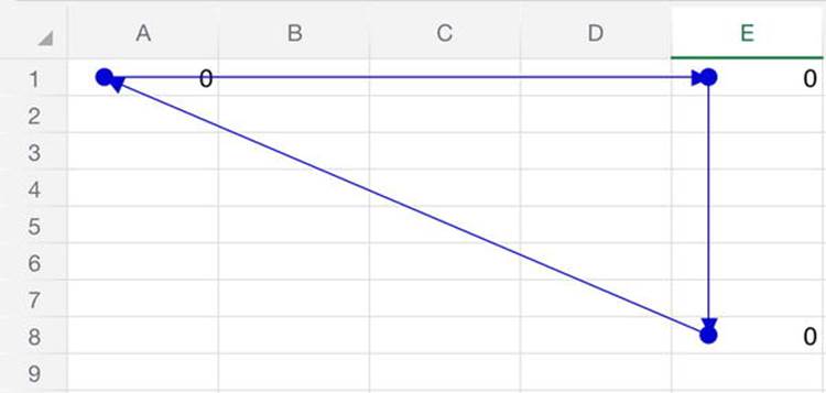
Figure 9-6. Excel displays arrows to indicate a circular reference among multiple cells
If you create a circular reference within a cell (making the cell refer to itself), Excel displays the Excel Cannot Calculate Formula dialog box (see Figure 9-7). Tap the OK button, and then remove the circular reference.
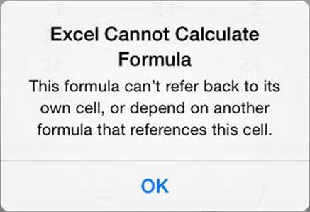
Figure 9-7. The Excel Cannot Calculate Formula dialog box warns you about a circular reference within a cell
Inserting Functions to Perform Standard Calculations
A function is a predefined formula for performing a standard calculation. Excel includes several hundred built-in functions that you can simply insert in a cell and provide with the data they need to deliver the result. Functions save you time and effort and help you avoid the mistakes that can occur when you create formulas. Excel also makes functions easy to use, so when you need to perform a standard calculation, check whether Excel has a function for it—most likely, it does.
In this section, you will learn how to insert functions into your worksheets, how to find the functions you want, and how to use arguments to give the functions the data they require for the calculations.
Once you’re comfortable with how functions work, I’ll review the different categories of functions that Excel provides, such as database functions, logical functions, and math and trigonometric functions. I’ll explain the functions you’re most likely to find useful, giving examples where they’ll be helpful.
Understanding Function Syntax
In Excel, a function has a name written in capitals followed by a pair of parentheses, which enclose any pieces of data the function needs. Here are three examples:
· SUM(): This widely used function adds together two or more values that you specify.
· COUNT(): This function counts the number of cells that contain numbers (as opposed to text, blanks, or other data types) in the range you specify.
· TODAY(): This function enters the current date in the cell.
Most functions take arguments, pieces of information that tell the function what you want it to work on. Excel’s two main tools for inserting functions, the Functions pop-up panel and the AutoSum Functions pop-up panel, both give you easy access to help information that lists the arguments required for each function.
To see the help about a function and a list of its arguments, follow these steps.
1. Double-tap the cell to open it for editing.
2. Tap the = key to display the Functions pop-up panel.
3. Locate the function you want to learn about.
4. Tap the Info button (the i button on the right of the function’s button) to display the Info panel. Figure 9-8 shows the Info panel for the AMORDEGRC function, which returns prorated linear depreciation of an asset.
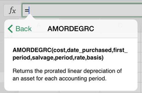
Figure 9-8. Open the Info panel for a function to see its argument list and a brief description of what it does
5. Tap the Back button to return to the Functions pop-up panel.
When you’ve identified the function you want to use, tap its button on the Functions pop-up panel to insert the function into the Formula bar. Excel displays the function’s arguments in gray boxes. For example, in Figure 9-9 the Formula bar shows the SUM() function. This function has one required argument and one optional argument, and you can add further arguments as needed:
· Required argument: Each required argument appears with its name in standard-weight type, like the argument number1 in the figure. You separate the arguments with commas, as in the example in the next paragraph. For example, you can use SUM() to add the values of cells in a range: SUM(C1:C10). Here, C1:C10 is a single argument, the required argument.
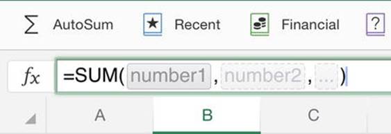
Figure 9-9. When you insert a function in the Formula bar, Excel displays a list of its arguments, showing which are required, which are optional, and whether you can use extra arguments
· Optional argument: Each optional argument appears in fainter type, like the argument [number2] in the figure. For example, you can use SUM() to add the values of two cells: SUM(C1,C3). Here, C1 is the required argument, and C3 is the first optional argument.
· Extra arguments: The ellipsis (…) shows that you can enter extra arguments of the same type. For example, you can use SUM() to add the values of many cells: SUM(C1,C3,D4,D8,E1,XF202). Here, C1 is the required argument, and all the other cell references are optional arguments.
Note Several functions take no arguments. For example, the TODAY() function simply returns the current date and requires no more information. Similarly, the NOW() function needs no arguments to return the current date and time, and the NA() function simply enters #(N/A) in a cell to indicate that the information is not available. But even when a function takes no arguments, you must include the parentheses to make Excel recognize the function.
Inserting a Function
You can insert a function in a worksheet either by using one of the Functions panels or by typing it the function into the cell. As you’ve seen, Excel automatically displays the main Functions panel when you type = to start creating a formula in a cell. But normally you’ll want to use the individual Functions panels, such as the AutoSum Functions panel or the Financial Functions panel, which you access from the Formulas tab of the Ribbon.
Inserting a Function Using the Functions Panels
To insert a function using one of the Functions panels, tap the Formulas tab of the Ribbon to display its controls (see Figure 9-10). You can then tap the button for the Functions panel you need.
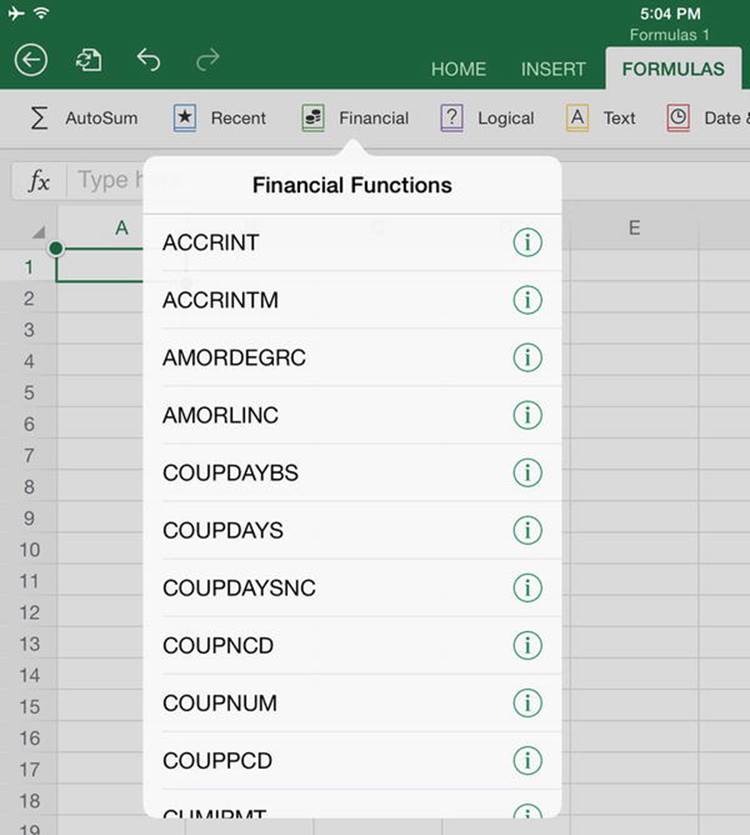
Figure 9-10. On the Formulas tab of the Ribbon, tap the button for the Functions panel you want to display. For example, tap the Financial button to display the Financial Functions panel
· AutoSum: This Functions panel enables you to enter the widely-used functions SUM(), AVERAGE(), COUNT(), MAX(), or MIN() in your worksheets.
Note In landscape orientation, the Formulas tab of the Ribbon displays the names of all the buttons except the More Functions button and the Recalculate button (the button at the right end). In portrait orientation, the Formulas tab displays the names of only the AutoSum button and the Recent button.
· Recent: This Functions panel provides quick access to the functions you’ve used most recently, enabling you to quickly insert a function again.
· Financial: This Functions panel contains functions for financial calculations—for example, calculating the payments on your mortgage or the depreciation on an asset.
· Logical: This Functions panel contains functions for performing logical tests—for example, testing whether a particular cell contains an error.
· Text: This Functions panel contains functions for manipulating text, such as the TRIM() function (for trimming off leading and trailing spaces) and the LEFT() function, which returns the leftmost part of the value.
· Date & Time: This Functions panel contains functions ranging from returning the current date with the TODAY() function to using the WEEKDAY() function to return the day of the week for a particular date.
· Lookup & Reference: This Functions panel contains functions for looking up data from other parts of a worksheet or referring to other cells in it.
· Math & Trigonometry: This Functions panel contains mathematical functions, such as the SQRT() function for returning a square root, and trigonometric functions, such as the ACOS() function for calculating the arccosine of a number.
· More Functions: (This is the … button to the right of the Math & Trigonometry button.) Tap this button to display the More Functions panel (see Figure 9-11), which gives you access to the following Functions panels:
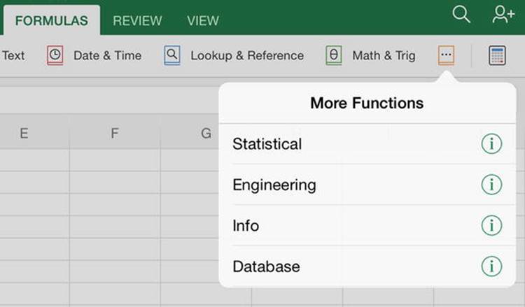
Figure 9-11. Open the More Functions panel to access the Statistical Functions panel, the Engineering Functions panel, the Info Functions panel, and the Database Functions panel
· Statistical: This category contains functions for performing statistical calculations, such as working out standard deviations based on a population or a sample.
· Engineering: This category contains functions including the DEC2HEX() function (for converting a decimal number to hexadecimal, base 16) and the HEX2OCT() function (for converting a hexadecimal number to octal, base 8).
· Information: This category contains functions for returning information about data, such as whether it is text or a number.
· Database: This category contains functions for working with databases—for example, returning the average of values in a column or list or the count of cells containing numbers in a field.
Tip If you want to browse the full list of functions in alphabetical order, double-tap the cell to open it for editing and then tap the = key on the onscreen keyboard to display the Functions panel. Scroll down past the Recently Used Functions list at the top to reach the All Functions list, where you can browse the functions.
When you find the function you need, tap it to insert it in the cell and in the Formula bar. Excel highlights the first required argument, and you can tap the cell that contains the value you want to use. Tap the next argument and then tap the appropriate cell (see the example in Figure 9-12). When you finish specifying the data to use for the function, tap the Enter button at the right end of the Formula bar to enter the function in the cell. The result then appears, and you can verify whether the formula is working.
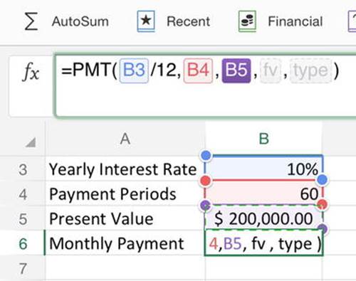
Figure 9-12. Tap an argument in the Formula bar and then tap the cell to use for the argument. Tap the Enter button to enter the function in the cell
Typing a Function Directly into a Cell
Typing a function into a cell works well when you know which function you want and you remember which arguments it requires. Usually, you’ll want to type in only simple functions, such as TODAY() or ROUND(), and take advantage of Excel’s help in entering other functions.
When you type the = sign to start the function, Excel displays the Functions pop-up panel. As you continue typing, the Functions pop-up panel narrows down the list to show only functions matching what you have typed. You can tap a function to insert it in the cell and the Formula bar with its arguments list or simply finish typing the function’s name; if you continue typing, Excel hides the Functions pop-up panel when you type the opening parenthesis for the function.
Nesting One Function Inside Another Function
Many calculations require only a single function, but for others, you will need to use multiple functions. You can combine functions as needed, using them in much the same way that you use values. For example, the AVERAGE() function calculates the average (the arithmetic mean) of the values of the arguments, so AVERAGE(1,2,3) returns 2; and the ROUND() function returns the value of the first argument rounded to the number of digits specified by the second argument, so ROUND(2.418, 0) returns 2. To add the results of the two functions together, you create a formula like this, giving the result 4:
=AVERAGE(1,2,3) + ROUND(2.418,0)
When you need one function to work on the value that a second function returns, you can nest that second function inside the first function. For example, if you need to return the current hour, you can nest the NOW() function in the HOUR() function. The NOW() function returns the current date and time, and the HOUR() function returns the hour from a given time (in 24-hour format; if you need the hour in AM/PM format, change the number format by tapping the cell, tapping the Number Formatting button, tapping the Info icon on the Time button, and then tapping the time format).
Here’s the NOW() function nested in the HOUR() function:
=HOUR(NOW())
As with formulas, you can nest functions many layers deep if you need to. Here’s an example with three layers of nesting:
=INT(AVERAGE(ROUND(SUM(C1:C6),2),ROUND(SUM(D1:D6),2)))
As explained earlier in this chapter, Excel starts by evaluating the most deeply nested expressions. Here’s what happens:
· SUM(C1:C6): This SUM function adds the values in the range C1:C6. Similarly, SUM(D1:D6) adds the values in the range D1:D6.
· ROUND(SUM(C1:C6),2): This ROUND function rounds the result of the SUM(C1:C6) formula to two decimal places. Similarly, ROUND(SUM(D1:D6),2) rounds the result of the SUM(D1:D6) formula to two decimal places.
· AVERAGE: This function returns the average of the results returned by the two ROUND functions.
· INT: This function returns the integer portion of the result from the AVERAGE function.
Meeting Excel’s Most Useful Functions
In this section, you meet 21 of Excel’s most widely useful functions. Excel has hundreds of functions, but many of them are highly specialized; for example, the AMORLINC function calculates an asset’s prorated linear depreciation for each accounting period in the French accounting system, and the BESSELJ function calculates the Bessel function Jn(x), also called cylindrical harmonics. Unless you work in French accounting or cylindrical harmonics or specialize in confusing your colleagues, chances are that you’ll use these functions seldom if ever.
By contrast, the 21 functions in this section turn up in a wide variety of workbooks, so you’ll likely use at least some of them.
SUM
The SUM function is so widely used that you’ll find it hard to avoid—and in fact you’ve already met it in this chapter. SUM calculates the sum of the specified numbers. For example, =SUM(1,2,3) returns 6.
AVERAGE, MEDIAN, and MODE
The AVERAGE function calculates the average of the specified values, cells, ranges, or arrays. For example, =AVERAGE(1,2,3) returns 2, and =AVERAGE(B1:B6) returns the average of the range B1:B6.
The MEDIAN function returns the median (the number in the middle of the given set) of the numbers or the values in the specified cells. For example, =MEDIAN(1,2,2,3,4,4,6) returns 3.
The MODE function returns the mode, the value that occurs most frequently in the specified values or range of cells. For example, =MODE(1,1,2,2,2,3,3,4,18) returns 2, because 2 is the number that occurs most frequently among the given numbers.
MAX and MIN
The MAX function returns the largest value in the specified range. For example, =MAX(C1:C6) returns the largest value in the range C1:C6.
The MIN function returns the smallest value in the specified range.
DAY, MONTH, and YEAR
The DAY function returns a serial number between 1 and 31, representing the day of the month for the specified serial date. For example, =DAY(42363) returns 25, indicating that the date falls on the 25th day in the month.
Similarly, the MONTH function returns a serial number between 1 and 12, representing the month in which the specified serial date falls. For example, =MONTH(42363) returns 12, indicating that the date is in December.
As you’d guess from the previous two functions, the YEAR function returns the four-digit number for the specified serial date. For example, =YEAR(42363) returns 2015, indicating that the date is in 2015.
IF
The IF function returns the first of the specified values if the condition is TRUE and the second of the specified values if the condition is FALSE. For example, =IF(HOUR(NOW())<12,"AM","PM") displays “AM” if the current hour is less than 12 and “PM” otherwise.
ISBLANK, NA, and ISNA
The ISBLANK function returns TRUE if the cell is blank and FALSE if it has contents. For example, =ISBLANK(A24) returns TRUE if cell A24 is blank.
The NA function causes a cell to display #(N/A). You use it to indicate that a value is not available.
The ISNA function returns TRUE if the specified cell contains #N/A, entered either via the NA function or as text, and FALSE if it doesn’t.
LEFT, RIGHT, and MID
The LEFT function returns the specified number of characters from the beginning of the text string. For example, =LEFT("Product Ratings",7) returns “Product.”
Similarly, the RIGHT function returns the specified number of characters from the end of specified text string. For example, =RIGHT("Product Ratings",7) returns “Ratings.”
In between LEFT and RIGHT, the MID function returns the specified number of characters after the starting point given in the specified text string. For example, =MID("Human Heart-Rate Monitor",7,10) returns “Heart-Rate.”
TRIM
The TRIM function gives you an easy way to remove unwanted spaces from text strings. TRIM returns the specified text string with spaces removed from the beginning and ends, and extra spaces between words removed to leave one space between words. For example, =TRIM( 4512 Christy Blvd. ) strips out the superfluous spaces and returns “4512 Christy Blvd.”
PI
The PI function returns the value of Pi to 15 digits (3.14159265358979).
ROUND, ROUNDDOWN, and ROUNDUP
The ROUND function returns the specified number rounded to the specified number of digits. For example, =ROUND(3.33333,2) returns 3.33.
The ROUNDDOWN function returns the specified number rounded down to the specified number of digits. For example, =ROUNDDOWN(18.57321,2) returns 18.57.
The ROUNDUP function returns the specified number rounded up to the specified number of digits. For example, =ROUNDUP(18.57321,2) returns 18.58.
Summary
In this chapter, you learned how to use formulas and functions to perform calculations in your workbooks. You know that a formula is the recipe for a calculation, and that a function is a preset formula built into Excel. You know how to put together a formula using an equal sign, cell or range references, operators, and other components. And you know how to insert functions in your worksheets and how to provide the arguments they require to work. You also met Excel’s most widely useful functions—at least, according to me.
All materials on the site are licensed Creative Commons Attribution-Sharealike 3.0 Unported CC BY-SA 3.0 & GNU Free Documentation License (GFDL)
If you are the copyright holder of any material contained on our site and intend to remove it, please contact our site administrator for approval.
© 2016-2026 All site design rights belong to S.Y.A.