Algorithms Third Edition in C++ Part 5. Graph Algorithms (2006)
CHAPTER EIGHTEEN
Graph Search
18.8 Generalized Graph Search
DFS and BFS are fundamental and essential graph-traversal methods that lie at the heart of numerous graph-processing algorithms. Knowing their essential properties, we now move to a higher level of abstraction, where we see that both methods are special cases of a generalized strategy for moving through a graph, one that is suggested by our BFS implementation (Program 18.9).
The basic idea is simple: We revisit our description of BFS from Section 18.6, but we use the term generic term fringe, instead of queue, to describe the set of edges that are possible candidates for being next added to the tree. We are led immediately to a general strategy for searching a connected component of a graph. Starting with a self-loop to a start vertex on the fringe and an empty tree, perform the following operation until the fringe is empty:
Move an edge from the fringe to the tree. If the vertex to which it leads is unvisited, visit that vertex, and put onto the fringe all edges that lead from that vertex to unvisited vertices.
This strategy describes a family of search algorithms that will visit all the vertices and edges of a connected graph,no matter what type of generalized queue we use to hold the fringe edges.
When we use a queue to implement the fringe, we get BFS, the topic of Section 18.6. When we use a stack to implement the fringe, we get DFS. Figure 18.25, which you should compare with Figures 18.6
Figure 18.25 Stack-based DFS
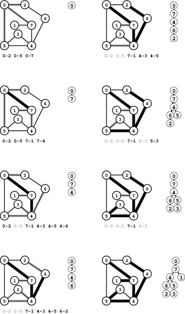
Together with Figure 18.21, this figure illustrates that BFS and DFS differ only in the underlying data structure. For BFS, we used a queue; for DFS we use a stack. We begin with all the edges adjacent to the start vertex on the stack (top left). Second, we move edge 0-7 from the stack to the tree and push onto the stack its incident edges that go to vertices not yet on the tree 7-1, 7-4, and 7-6 (second from top, left). The LIFO stack discipline implies that, when we put an edge on the stack, any edges that point to the same vertex are obsolete and will be ignored when they reach the top of the stack. Such edges are printed in gray. Third, we move edge 7-6 from the stack to the tree and push its incident edges on the stack (third from top, left). Next, we pop edge 4-6 and push its incident edges on the stack, two of which will take us to new vertices (bottom left). To complete the search, we take the remaining edges off the stack, completely ignoring the gray edges when they come to the top of the stack (right).
and 18.21, illustrates this phenomenon in detail. Proving this equivalence between recursive and stack-based DFS is an interesting exercise in recursion removal, where we essentially transform the stack underlying the recursive program into the stack implementing the fringe (see Exercise 18.63). The search order for the DFS depicted in Figure 18.25 differs from the one depicted in Figure 18.6 only because the stack discipline implies that we check the edges incident on each vertex in reverse of the order that we encounter them in the adjacency matrix (or the adjacency lists). The basic fact remains that, if we change the data structure used by Program 18.8 to be a stack instead of a queue (which is trivial to do because the ADT interfaces of the two data structures differ in only the function names), then we change that program from BFS to DFS.
Now, as we discussed in Section 18.7, this general method may not be as efficient as we would like, because the fringe becomes cluttered up with edges that point to vertices that are moved to the tree during the time that the edge is on the fringe. For FIFO queues, we avoid this situation by marking destination vertices when we put edges on the queue. We ignore edges to fringe vertices because we know that they will never be used: The old one will come off the queue (and the vertex visited) before the new one does (see Program 18.9). For a stack implementation, we want the opposite: When an edge is to be added to the fringe that has the same destination vertex as the one already there, we know that the old edge will never be used, because the new one will come off the stack (and the vertex visited) before the old one. To encompass these two extremes and to allow for fringe implementations that can use some other policy to disallow edges on the fringe that point to the same vertex, we modify our general scheme as follows:
Move an edge from the fringe to the tree. Visit the vertex that it leads to, and put all edges that lead from that vertex to unvisited vertices onto the fringe, using a replacement policy on the fringe that ensures that no two edges on the fringe point to the same vertex.
The no-duplicate-destination-vertex policy on the fringe guarantees that we do not need to test whether the destination vertex of the edge coming off the queue has been visited. For BFS, we use a queue implementation with an ignore-the-new-item policy; for DFS, we need
Figure 18.26 Graph search terminology
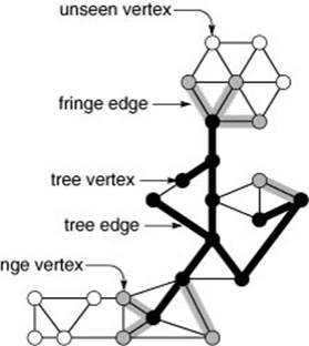
During a graph search, we maintain a search tree (black) and a fringe (gray) of edges that are candidates to be next added to the tree. Each vertex is either on the tree (black), the fringe (gray), or not yet seen (white). Tree vertices are connected by tree edges, and each fringe vertex is connected by a fringe edge to a tree vertex.
Figure 18.27 Graph search strategies
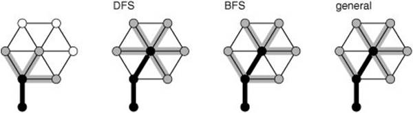
This figure illustrates different possibilities when we take a next step in the search illustrated in Figure 18.26. We move a vertex from the fringe to the tree (in the center of the wheel at the top right) and check all its edges, putting those to unseen vertices on the fringe and using an algorithm-specific replacement rule to decide whether those to fringe vertices should be skipped or should replace the fringe edge to the same vertex. In DFS, we always replace the old edges; in BFS, we always skip the new edges; and in other strategies, we might replace some and skip others.
a stack with a forget-the-old-item policy; but any generalized queue and any replacement policy at all will still yield an effective method for visiting all the vertices and edges of the graph in linear time and extra space proportional to V. Figure 18.27 is a schematic illustration of these differences. We have a family of graph-searching strategies that includes both DFS and BFS and whose members differ only in the generalized-queue implementation that they use. As we shall see, this family encompasses numerous other classical graph-processing algorithms.
Program 18.10 is an implementation based on these ideas for graphs represented with adjacency lists. It puts fringe edges on a generalized queue and uses the usual vertex-indexed vectors to identify fringe vertices so that it can use an explicit update ADT operation whenever it encounters another edge to a fringe vertex. The ADT implementation can choose to ignore the new edge or to replace the old one.
Property 18.12 Generalized graph searching visits all the vertices and edges in a graph in time proportional to V2for the adjacency-matrix representation and to V + E for the adjacency-lists representation plus, in the worst case, the time required for V insert, V remove, and E update operations in a generalized queue of size V.
Proof: The proof of Property 18.12 does not depend on the queue implementation, and therefore applies. The stated extra time requirements for the generalized-queue operations follow immediately from the implementation.
There are many other effective ADT designs for the fringe that we might consider. For example, as with our first BFS implementation, we could stick with our first general scheme and simply put all the edges on the fringe, then ignore those that go to tree vertices when
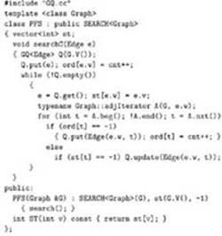
Program 18.10 Generalized graph search
This graph-search class generalizes BFS and DFS and supports numerous graph-processing algorithms (see Section 21.2 for a discussion of these algorithms and alternate implementations). It maintains a generalized queue of edges called the fringe. We initialize the fringe with a self-loop to the start vertex; then, while the fringe is not empty, we move an edge e from the fringe to the tree (attached at e.v) and scan e.w’s adjacency list, moving unseen vertices to the fringe and calling update for new edges to fringe vertices.
This code makes judicious use of ord and st to guarantee that no two edges on the fringe point to the same vertex. A vertex v is the destination vertex of a fringe edge if and only if it is marked (ord[v] is not -1) but it is not yet on the tree (st[v] is -1).
Program 18.11 Random queue implementation
When we remove an item from this data structure, it is equally likely to be any one of the items currently in the data structure. We can use this code to implement the generalized-queue ADT for graph searching to search a graph in a “random” fashion (see text).
template <class Item>
class GQ
{
private:
vector<Item> s; int N;
public:
GQ(int maxN) : s(maxN+1), N(0) { }
int empty() const
{ return N == 0; }
void put(Item item)
{ s[N++] = item; }
void update(Item x) { }
Item get()
{ int i = int(N*rand()/(1.0+RAND_MAX));
Item t = s[i];
s[i] = s[N-1];
s[N-1] = t;
return s[--N]; }
};
we take them off. The disadvantage of this approach, as with BFS, is that the maximum queue size has to be E instead of V. Or, we could handle updates implicitly in the ADT implementation, just by specifying that no two edges with the same destination vertex can be on the queue. But the simplest way for the ADT implementation to do so is essentially equivalent to using a vertex-indexed vector (see Exercises 4.51 and 4.54), so the test fits more comfortably into the client graph-search program.
The combination of Program 18.10 and the generalized-queue abstraction gives us a general and flexible graph-search mechanism. To illustrate this point, we now consider briefly two interesting and useful alternatives to BFS and DFS.
The first alternative strategy is based on randomized queues (see Section 4.6). In a randomized queue, we remove items randomly: Each item on the data structure is equally likely to be the one removed. Program 18.11 is an implementation that provides this functionality. If we use this code to implement the generalized queue ADT for Program 18.10, then we get a randomized graph-searching algorithm, where each vertex on the fringe is equally likely to be the next one added to the tree. The edge (to that vertex) that is added to the tree depends on the implementation of theupdate operation. The implementation in Program 18.11 does no updates, so each fringe vertex is added to the tree with the edge that caused it to be moved to the fringe. Alternatively, we might choose to always do updates (which results in the most recently encountered edge to each fringe vertex being added to the tree), or to make a random choice.
Another strategy, which is critical in the study of graph-processing algorithms because it serves as the basis for a number of the classical algorithms that we address in Chapters 20 through 22, is to use a priority-queue ADT (see Chapter 9) for the fringe: We assign priority values to each edge on the fringe, update them as appropriate, and choose the highest-priority edge as the one to be added next to the tree. We consider this formulation in detail in Chapter 20. The queue-maintenance operations for priority queues are more costly than are those for stacks and queues because they involve implicit comparisons among items on the queue, but they can support a much broader class of graph-search algorithms. As we shall see, several critical graph-processing problems can be addressed simply with judicious choice of priority assignments in a priority-queue–based generalized graph search.
All generalized graph-searching algorithms examine each edge just once and take extra space proportional to V in the worst case; they do differ, however, in some performance measures. For example, Figure 18.28 shows the size of the fringe as the search progresses for DFS, BFS, and randomized search; Figure 18.29 shows the tree computed by randomized search for the same example as Figure 18.13 and Figure 18.24. Randomized search has neither the long paths of DFS nor the high-degree nodes of BFS. The shapes of these trees and the fringe plots depend on the structure of the particular graph being searched, but they also characterize the different algorithms.
Figure 18.28 Fringe sizes for DFS, randomized graph search, and BFS
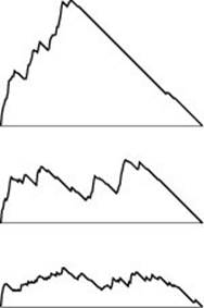
These plots of the fringe size during the searches illustrated in Figures 18.13, 18.24, and 18.29 indicate the dramatic effects that the choice of data structure for the fringe can have on graph searching. When we use a stack, in DFS (top), we fill up the fringe early in the search as we find new nodes at every step, then we end the search by removing everything. When we use a randomized queue (center), the maximum queue size is much lower. When we use a FIFO queue in BFS (bottom), the maximum queue size is still lower, and we discover new nodes throughout the search.
Figure 18.29 Randomized graph search
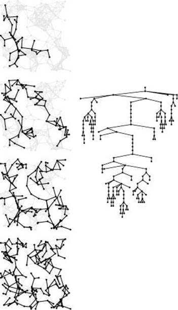
This figure illustrates the progress of randomized graph searching (left), in the same style as Figures 18.13 and 18.24. The search tree shape falls somewhere between the BFS and DFS shapes. The dynamics of these three algorithms, which differ only in the data structure for work to be completed, could hardly be more different.
We could generalize graph searching still further by working with a forest (not necessarily a tree) during the search. Although we stop short of working at this level of generality throughout, we consider a few algorithms of this sort in Chapter 20.
Exercises
• 18.61 Discuss the advantages and disadvantages of a generalized graph-searching implementation that is based on the following policy: “Move an edge from the fringe to the tree. If the vertex that it leads to is unvisited, visit that vertex and put all its incident edges onto the fringe.”
18.62 Develop an adjacency-lists ADT implementation that keeps edges (not just destination vertices) on the lists, then implement a graph search based on the strategy described in Exercise 18.61 that visits every edge but destroys the graph, taking advantage of the fact that you can move all of a vertex’s edges to the fringe with a single link change.
• 18.63 Prove that recursive DFS (Program 18.3) is equivalent to generalized graph search using a stack (Program 18.10), in the sense that both programs will visit all vertices in precisely the same order for all graphs if and only if the programs scan the adjacency lists in opposite orders.
18.64 Give three different possible traversal orders for randomized search through the graph
3-7 1-4 7-8 0-5 5-2 3-8 2-9 0-6 4-9 2-6 6-4.
18.65 Could randomized search visit the vertices in the graph
3-7 1-4 7-8 0-5 5-2 3-8 2-9 0-6 4-9 2-6 6-4
in numerical order of their indices? Prove your answer.
18.66 Use the STL to build a generalized-queue implementation for graph edges that disallows edges with duplicate vertices on the queue, using an ignore-the-new-item policy.
• 18.67 Develop a randomized graph search that chooses each edge on the fringe with equal likelihood. Hint: See Program 18.8.
• 18.68 Describe a maze-traversal strategy that corresponds to using a standard pushdown stack for generalized graph searching (see Section 18.1).
• 18.69 Instrument generalized graph searching (see Program 18.10) to print out the height of the tree and the percentage of edges processed for every vertex to be seen.
• 18.70 Run experiments to determine empirically the average values of the quantities described in Exercise 18.69 for generalized graph search with a random queue in graphs of various sizes, drawn from various graph models (see Exercises 17.64–76).
• 18.71 Implement a derived class that does dynamic graphical animations of generalized graph search for graphs that have (x, y) coordinates associated with each vertex (see Exercises 17.55 through 17.59). Test your program on random Euclidean neighbor graphs, using as many points as you can process in a reasonable amount of time. Your program should produce images like the snapshots shown in Figures 18.13, 18.24, and 18.29, although you should feel free to use colors instead of shades of gray to denote tree, fringe, and unseen vertices and edges.
All materials on the site are licensed Creative Commons Attribution-Sharealike 3.0 Unported CC BY-SA 3.0 & GNU Free Documentation License (GFDL)
If you are the copyright holder of any material contained on our site and intend to remove it, please contact our site administrator for approval.
© 2016-2025 All site design rights belong to S.Y.A.