Algorithms Third Edition in C++ Part 5. Graph Algorithms (2006)
CHAPTER NINETEEN
Digraphs and DAGs
19.5 DAGs
In this section, we consider various applications of directed acyclic graphs (DAGs). We have two reasons to do so. First, because they serve as implicit models for partial orders, we work directly with DAGs in many applications and need efficient algorithms to process them. Second, these various applications give us insight into the nature of DAGs, and understanding DAGs is essential to understanding general digraphs.
Since DAGs are a special type of digraph, all DAG-processing problems trivially reduce to digraph-processing problems. Although we expect processing DAGs to be easier than processing general di-graphs, we know when we encounter a problem that is difficult to solve on DAGs we should not expect to do any better solving the same problem on general digraphs. As we shall see, the problem of computing the transitive closure lies in this category. Conversely, understanding the difficulty of processing DAGs is important because every digraph has a kernel DAG (see Property 19.2), so we encounter DAGs even when we work with digraphs that are not DAGs.
The prototypical application where DAGs arise directly is called scheduling. Generally, solving scheduling problems has to do with arranging for the completion of a set of tasks, under a set of constraints, by specifying when and how the tasks are to be performed. Constraints might involve functions of the time taken or other resources consumed by the tasks. The most important type of constraints are precedence constraints, which specify that certain tasks must be performed before certain others, thus comprising a partial order among the tasks. Different types of additional constraints lead to many different types of scheduling problems, of varying difficulty. Literally thousands of different problems have been studied, and researchers still seek better algorithms for many of them. Perhaps the simplest nontrivial scheduling problem may be stated as follows:
Scheduling Given a set of tasks to be completed, with a partial order that specifies that certain tasks have to be completed before certain other tasks are begun, how can we schedule the tasks such that they are all completed while still respecting the partial order?
In this basic form, the scheduling problem is called topological sorting; it is not difficult to solve, as we shall see in the next section by examining two algorithms that do so. In more complicated practical applications, we might need to add other constraints on how the tasks might be scheduled, and the problem can become much more difficult. For example, the tasks might correspond to courses in a student’s schedule, with the partial order specifying prerequisites. Topological sorting gives a feasible course schedule that meets the prerequisite requirements, but perhaps not one that respects other constraints that need to be added to the model, such as course conflicts, limitations on enrollments, and so forth. As another example, the tasks might be part of a manufacturing process, with the partial order specifying sequential requirements of the particular process. Topological sorting gives us a way to schedule the tasks, but perhaps there is another way to do so that uses less time, money, or some other resources not included in the model. We examine versions of the scheduling problem that capture more general situations such as these inChapters 21 and 22.
Often, our first task is to check whether or not a given DAG indeed has no directed cycles. As we saw in Section 19.2, we can easily implement a class that allows clients to test whether a general digraph is a DAG in linear time, by running a standard DFS and checking that the DFS forest has no back edges (see Exercise 19.75). To implement DAG-specific algorithms, we implement task-specific client classes of our standard GRAPH ADT that assume they are processing digraphs with no cycles, leaving the client the responsibility of checking for cycles. This arrangement allows for the possibility that a DAG-processing algorithm produces useful results even when run on a digraph with cycles, which is sometimes the case. Sections 19.6 and 19.7 are devoted to implementations of classes for topological sorting (DAGts) and reachability in DAGs (DAGtc and DAGreach); Program 19.13 is an example of a client of such a class.
In a sense, DAGs are part tree, part graph. We can certainly take advantage of their special structure when we process them. For example, we can view a DAG almost as we view a tree, if we wish. Suppose that we want to traverse the vertices of the DAG D as though it were a tree rooted at w, so that, for example, the result of traversing the two DAGs in Figure 19.18 with this program would be the same. The following simple program accomplishes this task in the same manner as would a recursive tree traversal:
void traverseR(Dag D, int v)
{
visit(v);
typename Dag::adjIterator A(D, v);
for (int t = A.beg(); !A.end(); t = A.nxt())
traverseR(D, t);
}
We rarely use a full traversal of this kind, however, because we normally want to take advantage of the same economies that save space in a DAG to save time in traversing it (for example, by marking visited nodes in a normal DFS). The same idea applies to a search, where we make a recursive call for only one link incident on each vertex. In such an algorithm, the search cost will be the same for the DAG and the tree, but the DAG uses far less space.
Because they provide a compact way to represent trees that have identical subtrees, we often use DAGs instead of trees when we represent computational abstractions. In the context of algorithm design, the distinction between the DAG representation and the tree representation of a program in execution is the essential distinction behind dynamic programming (see, for example, Figure 19.18 and Exercise 19.78). DAGs are also widely used in compilers as intermediate representations of arithmetic expressions and programs (see, for example, Figure 19.19) and in circuit-design systems as intermediate representations of combinational circuits.
Along these lines, an important example that has many applications arises when we consider binary trees. We can apply the same restriction to DAGs that we applied to trees to define binary trees.
Definition 19.6 A binary DAG is a directed acyclic graph with two edges leaving each node, identified as the left edge and the right edge, either or both of which may be null.
Figure 19.18 DAG model of Fibonacci computation
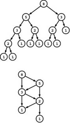
The tree at the top shows the dependence of computing each Fibonacci number on computing its two predecessors. The DAG at the bottom shows the same dependence with only a fraction of the nodes.
The distinction between a binary DAG and a binary tree is that in the binary DAG we can have more than one link pointing to a node. As did our definition for binary trees, this definition models a natural representation, where each node is a structure with a left link and a right link that point to other nodes (or are null), subject to only the global restriction that no directed cycles are allowed. Binary DAGs are significant because they provide a compact way to represent binary trees in certain applications. For example, we can compress an existence trie into a binary DAG without changing the search implementation, as shown Figure 19.20 and Program 19.5.
Figure 19.19 DAG representation of an arithmetic expression
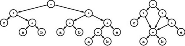
Both of these DAGs are representations of the arithmetic expression (c*(a+b))-((a+b))*((a+b)+e)). In the binary parse tree at left, leaf nodes represent operands and internal nodes each represent operators to be applied to the expressions represented by their two subtrees (see Figure 5.31). The DAG at right is a more compact representation of the same tree. More important, we can compute the value of the expression in time proportional to the size of the DAG, which is typically significantly less than the size of the tree (see Exercises 19.112 and 19.113).
An equivalent application is to view the trie keys as corresponding to rows in the truth table of a Boolean function for which the function is true (see Exercises 19.84 through 19.87). The binary DAG is a model for an economical circuit that computes the function. In this application, binary DAGs are known as binary decision diagrams (BDD) s.
Motivated by these applications, we turn, in the next two sections, to the study of DAG-processing algorithms. Not only do these algorithms lead to efficient and useful DAG ADT function implementations, but also they provide insight into the difficulty of processing digraphs. As we shall see, even though DAGs would seem to be substantially simpler structures than general digraphs, some basic problems are apparently no easier to solve.
Exercises
• 19.75 Implement a DFS class for use by clients for verifying that a DAG has no cycles.
• 19.76 Write a program that generates random DAGs by generating random digraphs, doing a DFS from a random starting point, and throwing out the back edges (see Exercise 19.40). Run experiments to decide how to set parameters in your program to expect DAGs with E edges, given V.
• 19.77 How many nodes are there in the tree and in the DAG corresponding to Figure 19.18 for FN, the Nth Fibonacci number?
19.78 Give the DAG corresponding to the dynamic-programming example for the knapsack model from Chapter 5 (see Figure 5.17).
• 19.79 Develop an ADT for binary DAGs.
Program 19.5 Representing a binary tree with a binary DAG
This code snippet is a postorder walk that constructs a compact representation of a binary DAG corresponding to a binary tree structure (see Chapter 12) by identifying common subtrees. It uses an indexing class like ST in Program 17.15 (modified to accept pairs of integer instead of string keys) to assign a unique integer to each distinct tree structure for use in representing the DAG as an vector of 2-integer structures (see Figure 19.20). The empty tree (null link) is assigned index 0, the single-node tree (node with two null links) is assigned index 1, and so forth.
The index corresponding to each subtree is computed recursively. Then a key is created such that any node with the same subtrees will have the same index and that index returned after the DAG’s edge (subtree) links are filled.
int compressR(link h)
{ STx st;
if (h == NULL) return 0;
l = compressR(h->l);
r = compressR(h->r);
t = st.index(l, r);
adj[t].l = l; adj[t].r = r;
return t;
}
Figure 19.20 Binary tree compression
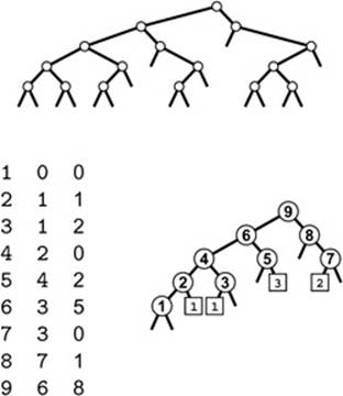
The table of nine pairs of integers at the bottom left is a compact representation of a binary DAG (bottom right) that is a compressed version of the binary tree structure at top. Node labels are not explicitly stored in the data structure: The table represents the eighteen edges 1-0, 1-0, 2-1, 2-1, 3-1, 3-2, and so forth, but designates a left edge and a right edge leaving each node (as in a binary tree) and leaves the source vertex for each edge implicit in the table index.
An algorithm that depends only upon the tree shape will work effectively on the DAG. For example, suppose that the tree is an existence trie for binary keys corresponding to the leaf nodes, so it represents the keys 0000, 0001, 0010, 0110, 1100, and 1101. A successful search for the key 1101 in the trie moves right, right, left, and right to end at a leaf node. In the DAG, the same search goes from 9 to 8 to 7 to 2 to 1.
• 19.80 Can every DAG be represented as a binary DAG (see Property 5.4)?
• 19.81 Write a function that performs an inorder traversal of a single-source binary DAG. That is, the function should visit all vertices that can be reached via the left edge, then visit the source, then visit all the vertices that can be reached via the right edge.
• 19.82 In the style of Figure 19.20, give the existence trie and corresponding binary DAG for the keys 01001010 10010101 00100001 11101100 01010001 00100001 00000111 01010011.
19.83 Implement an ADT based on building an existence trie from a set of 32-bit keys, compressing it as a binary DAG, then using that data structure to support existence queries.
• 19.84 Draw the BDD for the truth table for the odd parity function of four variables, which is 1 if and only if the number of variables that have the value 1 is odd.
19.85 Write a function that takes a 2n-bit truth table as argument and returns the corresponding BDD. For example, given the input 1110001000001100, your program should return a representation of the binary DAG in Figure 19.20.
19.86 Write a function that takes a 2n-bit truth table as argument, computes every permutation of its argument variables, and, using your solution to Exercise 19.85, finds the permutation that leads to the smallest BDD.
• 19.87 Run empirical studies to determine the effectiveness of the strategy of Exercise 19.87 for various Boolean functions, both standard and randomly generated.
19.88 Write a program like Program 19.5 that supports common subexpression removal: Given a binary tree that represents an arithmetic expression, compute a binary DAG that represents the same expression with common subexpressions removed.
• 19.89 Draw all the nonisomorphic DAGs with two, three, four, and five vertices.
••19.90 How many different DAGs are there with V vertices and E edges?
••• 19.91 How many different DAGs are there with V vertices and E edges, if we consider two DAGs to be different only if they are not isomorphic?
Figure 19.21 Topological sort (relabeling)
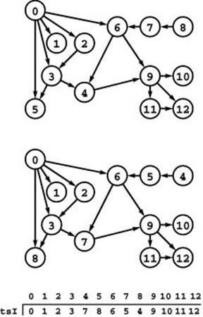
Given any DAG (top), topological sorting allows us to relabel its vertices so that every edge points from a lower-numbered vertex to a higher-numbered one (bottom). In this example, we relabel 4, 5, 7, and 8 to 7, 8, 5, and 4, respectively, as indicated in the array tsI. There are many possible labelings that achieve the desired result.
All materials on the site are licensed Creative Commons Attribution-Sharealike 3.0 Unported CC BY-SA 3.0 & GNU Free Documentation License (GFDL)
If you are the copyright holder of any material contained on our site and intend to remove it, please contact our site administrator for approval.
© 2016-2026 All site design rights belong to S.Y.A.