Algorithms Third Edition in C++ Part 5. Graph Algorithms (2006)
CHAPTER TWENTY-ONE
Shortest Paths
21.6 Reduction
It turns out that shortest-paths problems—particularly the general case, where negative weights are allowed (the topic of Section 21.7)—represent a general mathematical model that we can use to solve a variety of other problems that seem unrelated to graph processing. This model is the first among several such general models that we encounter. As we move to more difficult problems and increasingly general models, one of the challenges that we face is to characterize precisely relationships among various problems. Given a new problem, we ask whether we can solve it easily by transforming it to a problem that we know how to solve. If we place restrictions on the problem, will we be able to solve it more easily? To help answer such questions, we digress briefly in this section to discuss the technical language that we use to describe these types of relationships among problems.
Definition 21.3 We say that a problem A reduces to another problem B if we can use an algorithm that solves B to develop an algorithm that solves A, in a total amount of time that is, in the worst case, no more than a constant times the worst-case running time of the algorithm that solves B. We say that two problems are equivalent if they reduce to each other.
We postpone until Part 8 a rigorous definition of what it means to “use” one algorithm to “develop” another. For most applications, we are content with the following simple approach. We show that A reduces to B by demonstrating that we can solve any instance of A in three steps:
• Transform it to an instance of B.
• Solve that instance of B.
• Transform the solution of B to be a solution of A.
As long as we can perform the transformations (and solve B ) efficiently, we can solve A efficiently. To illustrate this proof technique, we consider two examples.
Property 21.12 The transitive-closure problem reduces to the all-pairs shortest-paths problem with nonnegative weights.
Figure 21.21 Transitive-closure reduction
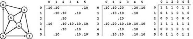
Given a digraph (left), we can transform its adjacency matrix (with self-loops) into an adjacency matrix representing a network by assigning an arbitrary weight to each edge (left matrix). As usual, blank entries in the matrix represent a sentinel value that indicates the absence of an edge. Given the all-pairs shortest-paths-lengths matrix of that network (center matrix), the transitive closure of the digraph (right matrix) is simply the matrix formed by subsituting 0 for each sentinel and 1 for all other entries.
Proof: We have already pointed out the direct relationship between Warshall’s algorithm and Floyd’s algorithm. Another way to consider that relationship, in the present context, is to imagine that we need to compute the transitive closure of digraphs using a library function that computes all shortest paths in networks. To do so, we add self-loops if they are not present in the digraph; then, we build a network directly from the adjacency matrix of the digraph, with an arbitrary weight (say 0.1) corresponding to each 1 and the sentinel weight corresponding to each 0. Then, we call the all-pairs shortest-paths function. Next, we can easily compute the transitive closure from the all-pairs shortest-paths matrix that the function computes: Given any two vertices u and v, there is a path from u to v in the digraph if and only if the length of the path from u to v in the network is nonzero (see Figure 21.21).
This property is a formal statement that the transitive-closure problem is no more difficult than the all-pairs shortest-paths problem. Since we happen to know algorithms for transitive closure that are even faster than the algorithms that we know for all-pairs shortest-paths problems, this information is no surprise. Reduction is more interesting when we use it to establish a relationship between problems that we do not know how to solve, or between such problems and other problems that we can solve.
Property 21.13 In networks with no constraints on edge weights, the longest-path and shortest-path problems (single-source or all-pairs) are equivalent.
Proof: Given a shortest-path problem, negate all the weights. A longest path (a path with the highest weight) in the modified network is a shortest path in the original network. An identical argument shows that the shortest-path problem reduces to the longest-path problem.
This proof is trivial, but this property also illustrates that care is justified in stating and proving reductions, because it is easy to take reductions for granted and thus to be misled. For example, it is decidedly not true that the longest-path and shortest-path problems are equivalent in networks with nonnegative weights.
At the beginning of this chapter, we outlined an argument that shows that the problem of finding shortest paths in undirected weighted graphs reduces to the problem of finding shortest paths in networks, so we can use our algorithms for networks to solve shortest-paths problems in undirected weighted graphs. Two further points about this reduction are worth contemplating in the present context. First, the converse does not hold: Knowing how to solve shortest-paths problems in undirected weighted graphs does not help us to solve them in networks. Second, we saw a flaw in the argument: If edge weights could be negative, the reduction gives networks with negative cycles, and we do not know how to find shortest paths in such networks. Even though the reduction fails, it turns out to be still possible to find shortest paths in undirected weighted graphs with no negative cycles with an unexpectedly complicated algorithm (see reference section). Since this problem does not reduce to the directed version, this algorithm does not help us to solve the shortest-path problem in general networks.
The concept of reduction essentially describes the process of using one ADT to implement another, as is done routinely by modern systems programmers. If two problems are equivalent, we know that if we can solve either of them efficiently, we can solve the other efficiently. We often find simple one-to-one correspondences, such as the one in Property 21.13, that show two problems to be equivalent. In this case, we have not yet discussed how to solve either problem, but it is useful to know that if we could find an efficient solution to one of them, we could use that solution to solve the other one. We saw another example in Chapter 17: When faced with the problem of determining whether or not a graph has an odd cycle, we noted that the problem is equivalent to determining whether or not the graph is two-colorable.
Reduction has two primary applications in the design and analysis of algorithms. First, it helps us to classify problems according to their difficulty at an appropriate abstract level without necessarily developing and analyzing full implementations. Second, we often do reductions to establish lower bounds on the difficulty of solving various problems, to help indicate when to stop looking for better algorithms. We have seen examples of these uses in Sections 19.3 and 20.7;we see others later in this section.
Beyond these direct practical uses, the concept of reduction also has widespread and profound implications for the theory of computation; these implications are important for us to understand as we tackle increasingly difficult problems. We discuss this topic briefly at the end of this section and consider it in full formal detail in Part 8.
The constraint that the cost of the transformations should not dominate is a natural one and often applies. In many cases, however, we might choose to use reduction even when the cost of the transformations does dominate. One of the most important uses of reduction is to provide efficient solutions to problems that might otherwise seem intractable by performing a transformation to a well-understood problem that we know how to solve efficiently. Reducing A to B, even if computing the transformations is much more expensive than is solving B, may give us a much more efficient algorithm for solving A than we could otherwise devise. There are many other possibilities. Perhaps we are interested in expected cost rather than the worst case. Perhaps we need to solve two problems B and C to solve A. Perhaps we need to solve multiple instances of B. We leave further discussion of such variations until Part 8, because all the examples that we consider before then are of the simple type just discussed.
In the particular case where we solve a problem A by simplifying another problem B, we know that A reduces to B, but not necessarily vice versa. For example, selection reduces to sorting because we can find the kth smallest element in a file by sorting the file and then indexing (or scanning) to the kth position, but this fact certainly does not imply that sorting reduces to selection. In the present context, the shortest-paths problem for weighted DAGs and the shortest-paths problem for networks with positive weights both reduce to the general shortest-paths problem. This use of reduction corresponds to the intuitive notion of one problem being more general than another. Any sorting algorithm solves any selection problem, and, if we can solve the shortest-paths problem in general networks, we certainly can use that solution for networks with various restrictions; but the converse is not necessarily true.
Figure 21.22 Job scheduling
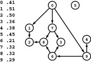
In this network, vertices represent jobs to be completed (with weights indicating the amount of time required) and edges represent precedence relationships between them. For example, the edges from 7 to 8 and 3 mean that job 7 must be finished before job 8 or job 3 can be started. What is the minimum amount of time required to complete all the jobs?
This use of reduction is helpful, but the concept becomes more useful when we use it to gain information about the relationships between problems in different domains. For example, consider the following problems, which seem at first blush to be far removed from graph processing. Through reduction, we can develop specific relationships between these problems and the shortest-paths problem.
Job scheduling A large set of jobs, of varying durations, needs to be performed. We can be working on any number of jobs at a given time, but a set of precedence relationships specify, for a set of pairs of jobs, that the first must be completed before the second can be started. What is the minimum amount of time required to complete all the jobs while satisfying all the precedence constraints? Specifically, given a set of jobs (with durations) and a set of precedence constraints, schedule the jobs (find a start time for each) so as to achieve this minimum.
Figure 21.22 depicts an example instance of the job-scheduling problem. It uses a natural network representation, which we use in a moment as the basis for a reduction. This version of the problem is perhaps the simplest of literally hundreds of versions that have been studied—versions that involve other job characteristics and other constraints, such as the assignment of personnel or other resources to the jobs, other costs associated with specific jobs, deadlines, and so forth. In this context, the version that we have described is commonly called precedence-constrained scheduling with unlimited parallelism; we use the term job scheduling as shorthand.
To help us to develop an algorithm that solves the job-scheduling problem, we consider the following problem, which is widely applicable in its own right.
Difference constraints Assign nonnegative values to a set variables x0 through xn that minimize the value of xn while satisfying a set of difference constraints on the variables, each of which specifies that the difference between two of the variables must be greater than or equal to a given constant.
Figure 21.23 depicts an example instance of this problem. It is a purely abstract mathematical formulation that can serve as the basis for solving numerous practical problems (see reference section).
The difference-constraint problem is a special case of a much more general problem where we allow general linear combinations of the variables in the equations.
Figure 21.23 Difference constraints
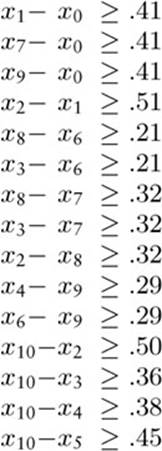
Finding an assignment of nonnegative values to the variables that minimizes the value of x10 subject to this set of inequalities is equivalent to the job-scheduling problem instance illustrated in Figure 21.22. For example, the equation x8x7 +. 32 means that job 8 cannot start until job 7 is completed.
Linear programming Assign nonnegative values to a set of variables x 0 through x n that minimize the value of a specified linear combination of the variables, subject to a set of constraints on the variables, each of which specifies that a given linear combination of the variables must be greater than or equal to a given constant.
Linear programming is a widely used general approach to solving a broad class of optimization problems that we will not consider it in detail until Part 8. Clearly, the difference-constraints problem reduces to linear programming, as do many other problems. For the moment, our interest is in the relationships among the difference-constraints, job-scheduling, and shortest-paths problems.
Property 21.14 The job-scheduling problem reduces to the difference-constraints problem.
Proof: Add a dummy job and a precedence constraint for each job saying that the job must finish before the dummy job starts. Given a job-scheduling problem, define a system of difference equations where each job i corresponds to a variable xi, and the constraint that j cannot start until i finishes corresponds to the equation xj ≥ xi + ci, where ci is the length of job i. The solution to the difference-constraints problem gives precisely a solution to the job-scheduling problem, with the value of each variable specifying the start time of the corresponding job.
Figure 21.23 illustrates the system of difference equations created by this reduction for the job-scheduling problem in Figure 21.22. The practical significance of this reduction is that we can use to solve job-scheduling problems any algorithm that can solve difference-constraint problems.
It is instructive to consider whether we can use this construction in the opposite way: Given a job-scheduling algorithm, can we use it to solve difference-constraints problems? The answer to this question is that the correspondence in the proof of Property 21.14 does not help us to show that the difference-constraints problem reduces to the job-scheduling problem, because the systems of difference equations that we get from job-scheduling problems have a property that does not necessarily hold in every difference-constraints problem. Specifically, if two equations have the same second variable, then they have the same constant. Therefore, an algorithm for job scheduling does not immediately give a direct way to solve a system of difference equations that contains two equations xi −xj ≥ a and xk − xj ≥ b, where a ≠ b. When proving reductions, we need to be aware of situations like this: A proof that A reduces to B must show that we can use an algorithm for solving B to solve any instance of A.
By construction, the constants in the difference-constraints problems produced by the construction in the proof of Property 21.14 are always nonnegative. This fact turns out to be significant.
Property 21.15 The difference-constraints problem with positive constants is equivalent to the single-source longest-paths problem in an acyclic network.
Proof: Given a system of difference equations, build a network where each variable xi corresponds to a vertex i and each equation xi xj c corresponds to an edge i-j of weight c. For example, assigning to each edge in the digraph of Figure 21.22 the weight of its source vertex gives the network corresponding to the set of difference equations in Figure 21.23. Add a dummy vertex to the network, with a zero-weight edge to every other vertex. If the network has a cycle, the system of difference equations has no solution (because the positive weights imply that the values of the variables corresponding to each vertex strictly decrease as we move along a path, and, therefore, a cycle would imply that some variable is less than itself), so report that fact. Otherwise, the network has no cycle, so solve the single-source longest-paths problem from the dummy vertex. There exists a longest path for every vertex because the network is acyclic (see Section 21.4). Assign to each variable the length of the longest path to the corresponding vertex in the network from the dummy vertex. For each variable, this path is evidence that its value satisfies the constraints and that no smaller value does so.
Unlike the proof of Property 21.14, this proof does extend to show that the two problems are equivalent because the construction works in both directions. We have no constraint that two equations with the same second variable in the equation must have the same constants, and no constraint that edges leaving any given vertex in the network must have the same weight. Given any acyclic network with positive weights, the same correspondence gives a system of difference constraints with positive constants whose solution directly yields a
Program 21.8 Job scheduling
This implementation reads a list of jobs with lengths followed by a list of precedence constraints from standard input, then prints on standard output a list of job starting times that satisfy the constraints. It solves the job-scheduling problem by reducing it to the longest-paths problem for acyclic networks, using Properties 21.14 and 21.15 and Program 21.6.
#include ”GRAPHbasic.cc“
#include ”GRAPHio.cc“
#include ”LPTdag.cc“
typedef WeightedEdge EDGE;
typedef DenseGRAPH<EDGE> GRAPH;
int main(int argc, char *argv[])
{ int i, s, t, N = atoi(argv[1]);
double duration[N];
GRAPH G(N, true);
for (int i = 0; i < N; i++)
cin >> duration[i];
while (cin >> s >> t)
G.insert(new EDGE(s, t, duration[s]));
LPTdag<GRAPH, EDGE> lpt(G);
for (i = 0; i < N; i++)
cout << i << ” “ << lpt.dist(i) << endl;
}
solution to the single-source longest-paths problem in the network. Details of this proof are left as an exercise (see Exercise 21.90).
The network in Figure 21.22 depicts this correspondence for our sample problem, and Figure 21.15 shows the computation of the longest paths in the network, using Program 21.6 (the dummy start vertex is implicit in the implementation). The schedule that is computed in this way is shown in Figure 21.24.
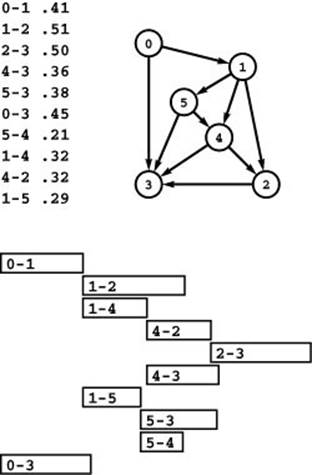
Figure 21.24 Job schedule
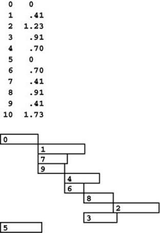
This figure illustrates the solution to the job-scheduling problem of Figure 21.22, derived from the correspondence between longest paths in weighted DAGs and job schedules. The longest path lengths in the wt array that is computed by the longest paths algorithm in Program 21.6 (seeFigure 21.15) are precisely the required job start times (top, right column). We start jobs 0 and 5 at time 0, jobs 1, 7, and 9 at time .41, jobs 4 and 6 at time .70, and so forth.
Program 21.8 is an implementation that shows the application of this theory in a practical setting. It transforms any instance of the job-scheduling problem into an instance of the longest-path problem in acyclic networks, then uses Program 21.6 to solve it.
We have been implicitly assuming that a solution exists for any instance of the job-scheduling problem; however, if there is a cycle in the set of precedence constraints, then there is no way to schedule the jobs to meet them. Before looking for longest paths, we should check for this condition by checking whether the corresponding network has a cycle (see Exercise 21.100). Such a situation is typical, and a specific technical term is normally used to describe it.
Definition 21.4 A problem instance that admits no solution is said to be infeasible.
In other words, for job-scheduling problems, the question of determining whether a job-scheduling problem instance is feasible reduces to the problem of determining whether a digraph is acyclic. As we move to ever-more-complicated problems, the question of feasibility becomes an ever-more-important (and ever-more-difficult!) part of our computational burden.
We have now considered three interrelated problems. We might have shown directly that the job-scheduling problem reduces to the single-source longest-paths problem in acyclic networks, but we have also shown that we can solve any difference-constraints problem (with positive constants) in a similar manner (see Exercise 21.94), as well as any other problem that reduces to a difference-constraints problem or a job-scheduling problem. We could, alternatively, develop an algorithm to solve the difference-constraints problem and use that algorithm to solve the other problems, but we have not shown that a solution to the job-scheduling problem would give us a way to solve the others.
These examples illustrate the use of reduction to broaden the applicability of proven implementations. Indeed, modern systems programming emphasizes the need to reuse software by developing new interfaces and using existing software resources to build implementations. This important process, which is sometimes referred to as library programming, is a practical realization of the idea of reduction.
Library programming is extremely important in practice, but it represents only part of the story of the implications of reduction. To illustrate this point, we consider the following version of the job-scheduling problem.
Job scheduling with deadlines Allow an additional type of constraint in the job-scheduling problem, to specify that a job must begin before a specified amount of time has elapsed, relative to another job. (Conventional deadlines are relative to the start job.) Such constraints are commonly needed in time-critical manufacturing processes and in many other applications, and they can make the job-scheduling problem considerably more difficult to solve.
Suppose that we need to add a constraint to our example of Figures 21.22 through 21.24 that job 2 must start earlier than a certain number c of time units after job 4 starts. If c is greater than .53, then the schedule that we have computed fits the bill, since it says to start job 2 at time 1.23, which is .53 after the end time of job 4 (which starts at .70). If c is less than .53, we can shift the start time of 4 later to meet the constraint. If job 4 were a long job, this change could increase the finish time of the whole schedule. Worse, if there are other constraints on job 4, we may not be able to shift its start time. Indeed, we may find ourselves with constraints that no schedule can meet: For instance, we could not satisfy a constraint in our example that job 2 must start earlier than d time units after the start of job 6 for d less than .53 because the constraints that 2 must follow 8 and 8 must follow 6 imply that 2 must start later than .53 time units after the start of 6.
If we add both of the two constraints described in the previous paragraph to the example, then both of them affect the time that 4 can be scheduled, the finish time of the whole schedule, and whether a feasible schedule exists, depending on the values of c and d. Adding more constraints of this type multiplies the possibilities and turns an easy problem into a difficult one. Therefore, we are justified in seeking the approach of reducing the problem to a known problem.
Property 21.16 The job-scheduling-with-deadlines problem reduces to the shortest-paths problem (with negative weights allowed).
Proof: Convert precedence constraints to inequalities using the same reduction described in Property 21.14. For any deadline constraint, add an inequality xi−x j ≤ dj, or, equivalently xj−xi≥−dj, where dj is a positive constant. Convert the set of inequalities to a network using the same reduction described in Property 21.15. Negate all the weights. By the same construction given in the proof of Property 21.15, any shortest-path tree rooted at 0 in the network corresponds to a schedule.
This reduction takes us to the realm of shortest paths with negative weights. It says that if we can find an efficient solution to the shortest-paths problem with negative weights, then we can find an efficient solution to the job-scheduling problem with deadlines. (Again, the correspondence in the proof of Property 21.16 does not establish the converse (see Exercise 21.91).)
Adding deadlines to the job-scheduling problem corresponds to allowing negative constants in the difference-constraints problem and negative weights in the shortest-paths problem. (This change also requires that we modify the difference-constraints problem to properly handle the analog of negative cycles in the shortest paths problem.) These more general versions of these problems are more difficult to solve than the versions that we first considered, but they are also likely to be more useful as more general models. A plausible approach to solving all of them would seem to be to seek an efficient solution to the shortest-paths problem with negative weights.
Unfortunately, there is a fundamental difficulty with this approach, and it illustrates the other part of the story in the use of reduction to assess the relative difficulty of problems. We have been using reduction in a positive sense, to expand the applicability of solutions to general problems; but it also applies in a negative sense, to show the limits on such expansion.
The difficulty is that the general shortest-paths problem is too hard to solve. We see next how the concept of reduction helps us to make this statement with precision and conviction. In Section 17.8, we discussed a set of problems, known as the NP-hard problems, that we consider to be intractable because all known algorithms for solving them require exponential time in the worst case. We show here that the general shortest-paths problem is NP-hard.
As mentioned briefly in Section 17.8 and discussed in detail in Part 8, we generally take the fact that a problem is NP-hard to mean not just that no efficient algorithm is known that is guaranteed to solve the problem but also that we have little hope of finding one. In this context, we use the term efficient to refer to algorithms whose running time is bounded by some polynomial function of the size of the input, in the worst case. We assume that the discovery of an efficient algorithm to solve any NP-hard problem would be a stunning research breakthrough. The concept of NP-hardness is important in identifying problems that are difficult to solve, because it is often easy to prove that a problem is NP-hard, using the following technique.
Property 21.17 A problem is NP-hard if there is an efficient reduction to it from any NP-hard problem.
This property depends on the precise meaning of an efficient reduction from one problem A to another problem B. We defer such definitions to Part 8 (two different definitions are commonly used). For the moment, we simply use the term to cover the case where we have efficient algorithms both to transform an instance of A to an instance of B and to transform a solution of B to a solution of A.
Now, suppose that we have an efficient reduction from an NP-hard problem A to a given problem B. The proof is by contradiction: If we have an efficient algorithm for B, then we could use it to solve any instance of A in polynomial time, by reduction (transform the given instance of A to an instance of B, solve that problem, then transform the solution). But no known algorithm can make such a guarantee for A (because A is NP-hard), so the assumption that there exists a polynomial-time algorithm for B is incorrect: B is also NP-hard.
This technique is extremely important because people have used it to show a huge number of problems to be NP-hard, giving us a broad variety of problems from which to choose when we want to develop a proof that a new problem is NP-hard. For example, we encountered one of the classic NP-hard problems in Section 17.7. The Hamilton-path problem, which asks whether there is a simple path containing all the vertices in a given graph, was one of the first problems shown to be NP-hard (see reference section). It is easy to formulate as a shortest-paths problem, so Property 21.17 implies that the shortest-paths problem itself is NP-hard:
Property 21.18 In networks with edge weights that could be negative, shortest-paths problems are NP-hard.
Proof: Our proof consists of reducing the Hamilton-path problem to the shortest-paths problem. That is, we show that we could use any algorithm that can find shortest paths in networks with negative edge weights to solve the Hamilton-path problem. Given an undirected graph, we build a network with edges in both directions corresponding to each edge in the graph and with all edges having weight −1. The shortest (simple) path starting at any vertex in this network is of length 1 − V if and only if the graph has a Hamilton path. Note that this network is replete with negative cycles. Not only does every cycle in the graph correspond to a negative cycle in the network, but also every edge in the graph corresponds to a cycle of weight −2 in the network.
The implication of this construction is that the shortest-paths problem is NP-hard, because if we could develop an efficient algorithm for the shortest-paths problem in networks, then we would have an efficient algorithm for the Hamilton-path problem in graphs.
One response to the discovery that a given problem is NP-hard is to seek versions of that problem that we can solve. For shortest-paths problems, we are caught between having a host of efficient algorithms for acyclic networks or for networks in which edge weights are nonnegative and having no good solution for networks that could have cycles and negative weights. Are there other kinds of networks that we can address? That is the subject of Section 21.7. There, for example, we see that the job-scheduling-with-deadlines problem reduces to a version of the shortest-paths problem that we can solve efficiently. This situation is typical: As we address ever-more-difficult computational problems, we find ourselves working to identify the versions of those problems that we can expect to solve.
As these examples illustrate, reduction is a simple technique that is helpful in algorithm design, and we use it frequently. Either we can solve a new problem by proving that it reduces to a problem that we know how to solve, or we can prove that the new problem will be difficult by proving that a problem that we know to be difficult reduces to the problem in question.
Table 21.3 gives us a more detailed look at the various implications of reduction results among the four general problem classes that we discussed in Chapter 17. Note that there are several cases where a reduction provides no new information; for example, although selection reduces to sorting and the problem of finding longest paths in acyclic networks reduces to the problem of finding shortest paths in general networks, these facts shed no new light on the relative difficulty of the problems. In other cases, the reduction may or may not provide new information; in still other cases, the implications of a reduction are truly profound. To develop these concepts, we need a precise and formal description of reduction, as we discuss in detail in Part 8; here, we summarize informally the most important uses of reduction in practice, with examples that we have already seen.
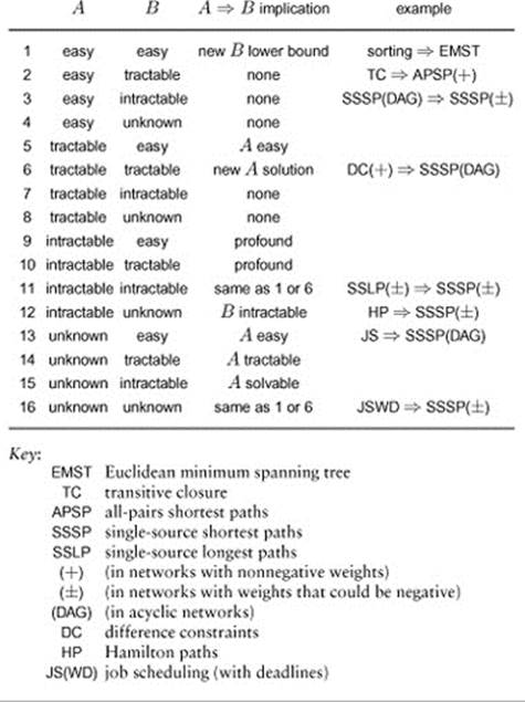
Table 21.3 Reduction implications
This table summarizes some implications of reducing a problem A to another problem B, with examples that we have discussed in this section. The profound implications of cases 9 and 10 are so far-reaching that we generally assume that it is not possible to prove such reductions (see Part 8). Reduction is most useful in cases 1, 6, 11, and 16, to learn a new algorithm for A or prove a lower bound on B; in cases 13-15, to learn new algorithms for A; and in case 12, to learn the difficulty of B.
Upper bounds If we have an efficient algorithm for a problem B and can prove that A reduces to B, then we have an efficient algorithm for A. There may exist some other better algorithm for A, but B’s performance is an upper bound on the best that we can do for A. For example, our proof that job scheduling reduces to longest paths in acyclic networks makes our algorithm for the latter an efficient algorithm for the former.
Lower bounds If we know that any algorithm for problem A has certain resource requirements and we can prove that A reduces to B, then we know that B has at least those same resource requirements, because a better algorithm for B would imply the existence of a better algorithm for A (as long as the cost of the reduction is lower than the cost of B). That is, A’s performance is a lower bound on the best that we can do for B. For example, we used this technique in Section 19.3 to show that computing the transitive closure is as difficult as Boolean matrix multiplication, and we used it in Section 20.7 to show that computing the Euclidean MST is as difficult as sorting.
Intractability In particular, we can prove a problem to be intractable by showing that an intractable problem reduces to it. For example, Property 21.18 shows that the shortest-paths problem is intractable because the Hamilton-path problem reduces to the shortest-paths problem.
Beyond these general implications, it is clear that more detailed information about the performance of specific algorithms to solve specific problems can be directly relevant to other problems that reduce to the first ones. When we find an upper bound, we can analyze the associated algorithm, run empirical studies, and so forth to determine whether it represents a better solution to the problem. When we develop a good general-purpose algorithm, we can invest in developing and testing a good implementation and then develop associated ADTs that expand its applicability.
We use reduction as a basic tool in this and the next chapter. We emphasize the general relevance of the problems that we consider, and the general applicability of the algorithms that solve them, by reducing other problems to them. It is also important to be aware of a hierarchy among increasingly general problem-formulation models. For example, linear programming is a general formulation that is important not just because many problems reduce to it but also because it is not known to be NP-hard. In other words, there is no known way to reduce the general shortest-paths problem (or any other NP-hard problem) to linear programming. We discuss such issues in Part 8.
Not all problems can be solved, but good general models have been devised that are suitable for broad classes of problems that we do know how to solve. Shortest paths in networks is our first example of such a model. As we move to ever-more-general problem domains, we enter the field ofoperations research (OR), the study of mathematical methods of decision making, where developing and studying such models is central. One key challenge in OR is to find the model that is most appropriate for solving a problem and to fit the problem to the model. This activity is sometimes known as mathematical programming (a name given to it before the advent of computers and the new use of the word “programming”). Reduction is a modern concept that is in the same spirit as mathematical programming and is the basis for our understanding of the cost of computation in a broad variety of applications.
Exercises
• 21.85 Use the reduction of Property 21.12 to develop a transitive-closure implementation (with the same interface as Programs 19.3 and 19.4) that uses the all-pairs shortest-paths ADT of Section 21.3.
21.86 Show that the problem of computing the number of strong components in a digraph reduces to the all-pairs shortest-paths problem with nonnegative weights.
21.87 Give the difference-constraints and shortest-paths problems that correspond—according to the constructions of Properties 21.14 and 21.15—to the job-scheduling problem, where jobs 0 to 7 have lengths
.4 .2 .3 .4 .2 .5 .1
and constraints
5-1 4-6 6-0 3-2 6-1 6-2,
respectively.
• 21.88 Give a solution to the job-scheduling problem of Exercise 21.87.
• 21.89 Suppose that the jobs in Exercise 21.87 also have the constraints that job 1 must start before job 6 ends, and job 2 must start before job 4 ends. Give the shortest-paths problem to which this problem reduces, using the construction described in the proof of Property 21.16.
21.90 Show that the all-pairs longest-paths problem in acyclic networks with positive weights reduces to the difference-constraints problem with positive constants.
• 21.91 Explain why the correspondence in the proof of Property 21.16 does not extend to show that the shortest-paths problem reduces to the job-scheduling-with-deadlines problem.
21.92 Extend Program 21.8 to use symbolic names instead of integers to refer to jobs (see Program 17.10).
21.93 Design an ADT interface that provides clients with the ability to pose and solve difference-constraints problems.
21.94 Write a class that implements your interface from Exercise 21.93, basing your solution to the difference-constraints problem on a reduction to the shortest-paths problem in acyclic networks.
21.95 Provide an implementation for a class that solves the single-source shortest-paths problem in acyclic networks with negative weights, which is based on a reduction to the difference-constraints problem and uses your interface from Exercise 21.93.
• 21.96 Your solution to the shortest-paths problem in acyclic networks for Exercise 21.95 assumes the existence of an implementation that solves the difference-constraints problem. What happens if you use the implementation from Exercise 21.94, which assumes the existence of an implementation for the shortest-paths problem in acyclic networks?
• 21.97 Prove the equivalence of any two NP-hard problems (that is, choose two problems and prove that they reduce to each other).
•• 21.98 Give an explicit construction that reduces the shortest-paths problem in networks with integer weights to the Hamilton-path problem.
• 21.99 Use reduction to implement a class that uses a network ADT that solves the single-source shortest-paths problem to solve the following problem: Given a digraph, a vertex-indexed vector of positive weights, and a start vertex v, find the paths from v to each other vertex such that the sum of the weights of the vertices on the path is minimized.
• 21.100 Program 21.8 does not check whether the job-scheduling problem that it takes as input is feasible (has a cycle). Characterize the schedules that it prints out for infeasible problems.
21.101 Design an ADT interface that gives clients the ability to pose and solve job-scheduling problems. Write a class that implements your interface, basing your solution to the job-scheduling problem on a reduction to the shortest-paths problem in acyclic networks, as in Program 21.8.
• 21.102 Add a function to your class from Exercise 21.101 (and provide an implementation) that prints out a longest path in the schedule. (Such a path is known as a critical path.)
21.103 Write a client for your interface from Exercise 21.101 that outputs a PostScript program that draws the schedule in the style of Figure 21.24 (see Section 4.3).
• 21.104 Develop a model for generating job-scheduling problems. Use this model to test your implementations of Exercises 21.101 and 21.103 for a reasonable set of problem sizes.
21.105 Write a class that implements your interface from Exercise 21.101, basing your solution to the job-scheduling problem on a reduction to the difference-constraints problem.
• 21.106 A PERT (performance-evaluation-review-technique) chart is a network that represents a job-scheduling problem, with edges representing jobs, as described in Figure 21.25. Write a class that implements your job-scheduling interface of Exercise 21.101 that is based on PERT charts.
21.107 How many vertices are there in a PERT chart for a job-scheduling problem with V jobs and E constraints?
21.108 Write programs to convert between the edge-based job-scheduling representation (PERT chart) discussed in Exercise 21.106 and the vertex-based representation used in the text (see Figure 21.22).
Figure 21.25 A PERT chart
A PERT chart is a network representation for job-scheduling problems where we represent jobs by edges. The network at the top is a representation of the job-scheduling problem depicted in Figure 21.22, where jobs 0 through 9 in Figure 21.22 are represented by edges 0-1, 1-2, 2-3, 4-3, 5-3, 0-3, 5-4, 1-4, 4-2, and 1-5, respectively, here. The critical path in the schedule is the longest path in the network.
All materials on the site are licensed Creative Commons Attribution-Sharealike 3.0 Unported CC BY-SA 3.0 & GNU Free Documentation License (GFDL)
If you are the copyright holder of any material contained on our site and intend to remove it, please contact our site administrator for approval.
© 2016-2026 All site design rights belong to S.Y.A.