Algorithms Third Edition in C++ Part 5. Graph Algorithms (2006)
CHAPTER TWENTY-ONE
Shortest Paths
21.7 Negative Weights
We now turn to the challenge of coping with negative weights in shortest-paths problems. Perhaps negative edge weights seem unlikely, given our focus through most of this chapter on intuitive examples, where weights represent distances or costs; however, we also saw in Section 21.6 that negative edge weights arise in a natural way when we reduce other problems to shortest-paths problems. Negative weights are not merely a mathematical curiosity; on the contrary, they significantly extend the applicability of the shortest-paths problems as a model for solving other problems. This potential utility is our motivation to search for efficient algorithms to solve network problems that involve negative weights.
Figure 21.26 is a small example that illustrates the effects of introducing negative weights on a network’s shortest paths. Perhaps the most important effect is that when negative weights are present, low-weight shortest paths tend to have more edges than higher-weight paths. For positive weights, our emphasis was on looking for shortcuts; but when negative weights are present, we seek detours that use as many edges with negative weights as we can find. This effect turns our intuition in seeking “short” paths into a liability in understanding the algorithms, so we need to suppress that line of intuition and consider the problem on a basic abstract level.
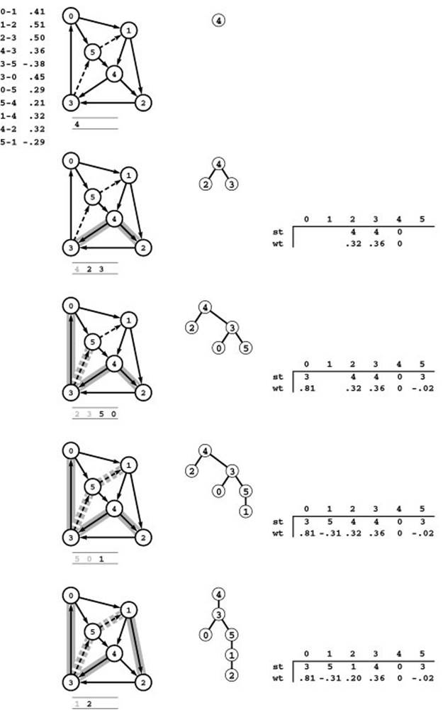
Figure 21.26 A sample network with negative edges
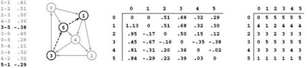
This sample network is the same as the network depicted in Figure 21.1, except that the edges 3-5 and 5-1 are negative. Naturally, this change dramatically affects the shortest paths structure, as we can easily see by comparing the distance and path matrices at the right with their counterparts in Figure 21.9. For example, the shortest path from 0 to 1 in this network is 0-5-1, which is of length 0; and the shortest path from 2 to 1 is 2-3-5-1, which is of length -.17.
The relationship shown in the proof of Property 21.18 between shortest paths in networks and Hamilton paths in graphs ties in with our observation that finding paths of low weight (which we have been calling “short”) is tantamount to finding paths with a high number of edges (which we might consider to be “long”). With negative weights, we are looking for long paths rather than short paths.
The first idea that suggests itself to remedy the situation is to find the smallest (most negative) edge weight, then to add the absolute value of that number to all the edge weights to transform the network into one with no negative weights. This naive approach does not work at all, because shortest paths in the new network bear little relation to shortest paths in the old one. For example, in the network illustrated in Figure 21.26, the shortest path from 4 to 2 is 4-3-5-1-2. If we add .38 to all the edge weights in the graph to make them all positive, the weight of this path grows from .20 to 1.74. But the weight of 4-2 grows from .32 to just .70, so that edge becomes the shortest path from 4 to 2. The more edges a path has, the more it is penalized by this transformation; that result, from the observation in the previous paragraph, is precisely the opposite of what we need. Even though this naive idea does not work, the goal of transforming the network into an equivalent one with no negative weights but the same shortest paths is worthy; at the end of the section, we consider an algorithm that achieves this goal.
Our shortest-paths algorithms to this point have all placed one of two restrictions on the shortest-paths problem so that they can offer an efficient solution: They either disallow cycles or disallow negative weights. Is there a less stringent restriction that we could impose on networks that contain both cycles and negative weights that would still lead to tractable shortest-paths problems? We touched on an answer to this question at the beginning of the chapter, when we had to add the restriction that paths be simple so that the problem would make sense if there were negative cycles. Should we perhaps restrict attention to networks that have no such cycles?
Shortest paths in networks with no negative cycles Given a network that may have negative edge weights but does not have any negative-weight cycles, solve one of the following problems: Find a shortest path connecting two given vertices (shortest-path problem), find shortest paths from a given vertex to all the other vertices (single-source problem), or find shortest paths connecting all pairs of vertices (all-pairs problem).
The proof of Property 21.18 leaves the door open for the possibility of efficient algorithms for solving this problem because it breaks down if we disallow negative cycles. To solve the Hamilton-path problem, we would need to be able to solve shortest-paths problems in networks that have huge numbers of negative cycles.
Moreover, many practical problems reduce precisely to the problem of finding shortest paths in networks that contain no negative cycles. We have already seen one such example.
Property 21.19 The job-scheduling-with-deadlines problem reduces to the shortest-paths problem in networks that contain no negative cycles.
Proof: The argument that we used in the proof of Property 21.15 shows that the construction in the proof of Property 21.16 leads to networks that contain no negative cycles. From the job-scheduling problem, we construct a difference-constraints problem with variables that correspond to job start times; from the difference-constraints problem, we construct a network. We negate all the weights to convert from a longest-paths problem to a shortest-paths problem—a transformation that corresponds to reversing the sense of all the inequalities. Any simple path from i to j in the network corresponds to a sequence of inequalities involving the variables. The existence of the path implies, by collapsing these inequalities, that xi − xj ≤ wij, where wij is the sum of the weights on the path from i to j. A negative cycle corresponds to 0 on the left side of this inequality and a negative value on the right, so the existence of such a cycle is a contradiction. •
Figure 21.27 Arbitrage
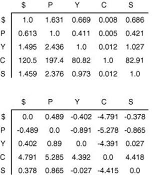
The table at the top specifies conversion factors from one currency to another. For example, the second entry in the top row says that $1 buys 1.631 units of currency P. Converting $1000 to currency P and back again would yield $1000*(1.631)*(0.613) = $999, a loss of $1. But converting $1000 to currency P then to currency Y and back again yields $1000*(1.631)*(0.411)*(1.495) = $1002, a .2% arbitrage opportunity. If we take the negative of the logarithm of all the numbers in the table (bottom), we can consider it to be the adjacency matrix for a complete network with edge weights that could be positive or negative. In this network, nodes correspond to currencies, edges to conversions, and paths to sequences of conversions. The conversion just described corresponds to the cycle $-P-Y-$ in the graph, which has weight −0.489 + 0.890 − 0.402 =. 002. The best arbitrage opportunity is the shortest cycle in the graph.
As we noted when we first discussed the job-scheduling problem in Section 21.6, this statement implicitly assumes that our job-scheduling problems are feasible (have a solution). In practice, we would not make such an assumption, and part of our computational burden would be determining whether or not a job-scheduling-with-deadlines problem is feasible. In the construction in the proof of Property 21.19, a negative cycle in the network implies an infeasible problem, so this task corresponds to the following problem.
Negative cycle detection Does a given network have a negative cycle? If it does, find one such cycle.
On the one hand, this problem is not necessarily easy (a simple cycle-checking algorithm for digraphs does not apply); on the other hand, it is not necessarily difficult (the reduction of Property 21.16 from the Hamilton-path problem does not apply). Our first challenge will be to develop an algorithm for this task.
In the job-scheduling-with-deadlines application, negative cycles correspond to error conditions that are presumably rare, but for which we need to check. We might even develop algorithms that remove edges to break the negative cycle and iterate until there are none. In other applications, detecting negative cycles is the prime objective, as in the following example.
Arbitrage Many newspapers print tables showing conversion rates among the world’s currencies (see, for example, Figure 21.27). We can view such tables as adjacency-matrix representations of complete networks. An edge s-t with weight x means that we can convert 1 unit of currency s into x units of currency t. Paths in the network specify multistep conversions. For example, if there is also an edge t-w with weight y, then the path s-t-w represents a way to convert 1 unit of currency s into xy units of currency w. We might expect xy to be equal to the weight of s-w in all cases, but such tables represent a complex dynamic system where such consistency cannot be guaranteed. If we find a case where xy is smaller than the weight of s-w, then we may be able to outsmart the system. Suppose that the weight of w-s is z and xyz > 1, then the cycle s-t-w-s gives a way to convert 1 unit of currency s into more than 1 units (xyz) of currency s. That is, we can make a 100(xyz − 1) percent profit by converting from s to t to w back to s. This situation is an example of an arbitrage opportunity that would allow us to make unlimited profits were it not for forces outside the model, such as limitations on the size of transactions. To convert this problem to a shortest-paths problem, we take the logarithm of all the numbers so that path weights correspond to adding edge weights instead of multiplying them, and then we take the negative to invert the comparison. Then the edge weights might be negative or positive, and a shortest path from s to t gives a best way of converting from currency s to currency t. The lowest-weight cycle is the best arbitrage opportunity, but any negative cycle is of interest.
Figure 21.28 Failure of Dijkstra’s algorithm (negative weights)
In this example, Dijkstra’s algorithm decides that 4-2 is the shortest path from 4 to 2 (of length .32) and misses the shorter path 4-3-5-1-2 (of length .20).
Can we detect negative cycles in a network or find shortest paths in networks that contain no negative cycles? The existence of efficient algorithms to solve these problems does not contradict the NP-hardness of the general problem that we proved in Property 21.18, because no reduction from the Hamilton-path problem to either problem is known. Specifically, the reduction of Property 21.18 says that what we cannot do is to craft an algorithm that can guarantee to find efficiently the lowest-weight path in any given network when negative edge weights are allowed. That problem statement is too general. But we can solve the restricted versions of the problem just mentioned, albeit not as easily as we can the other restricted versions of the problem (positive weights and acyclic networks) that we studied earlier in this chapter.
In general, as we noted in Section 21.2, Dijkstra’s algorithm does not work in the presence of negative weights, even when we restrict attention to networks that contain no negative cycles. Figure 21.28 illustrates this fact. The fundamental difficulty is that the algorithm depends on examining paths in increasing order of their length. The proof that the algorithm is correct (see Property 21.2) assumes that adding an edge to a path makes that path longer.
Floyd’s algorithm makes no such assumption and is effective even when edge weights may be negative. If there are no negative cycles, it computes shortest paths; remarkably enough, if there are negative cycles, it detects at least one of them.
Property 21.20 Floyd’s algorithm solves the negative-cycle–detection problem and the all-pairs shortest-paths problem in networks that contain no negative cycles, in time proportional to V3.
Proof: The proof of Property 21.8 does not depend on whether or not edge weights are negative; however, we need to interpret the results differently when negative edge weights are present. Each entry in the matrix is evidence of the algorithm having discovered a path of that length; in particular, any negative entry on the diagonal of the distances matrix is evidence of the presence of at least one negative cycle. In the presence of negative cycles, we cannot directly infer any further information, because the paths that the algorithm implicitly tests are not necessarily simple: Some may involve one or more trips around one or more negative cycles. However, if there are no negative cycles, then the paths that are computed by the algorithm are simple, because any path with a cycle would imply the existence of a path that connects the same two points which has fewer edges and is not of higher weight (the same path with the cycle removed).
The proof of Property 21.20 does not give specific information about how to find a specific negative cycle from the distances and paths matrices computed by Floyd’s algorithm. We leave that task for an exercise (see Exercise 21.122).
Floyd’s algorithm solves the all-pairs shortest-paths problem for graphs that contain no negative cycles. Given the failure of Dijkstra’s algorithm in networks that contain weights that could be negative, we could also use Floyd’s algorithm to solve the the all-pairs problem for sparse networks that contain no negative cycles, in time proportional to V3. If we have a single-source problem in such networks, then we can use this V3 solution to the all-pairs problem that, although it amounts to overkill, is the best that we have yet seen for the single-source problem. Can we develop faster algorithms for these problems—ones that achieve the running times that we achieve with Dijkstra’s algorithm when edge weights are positive (E lg V for single-source shortest paths and V E lg V for all-pairs shortest paths)? We can answer this question in the affirmative for the all-pairs problem and also can bring down the worst-case cost to V E for the single-source problem, but breaking the V E barrier for the general single-source shortest-paths problem is a longstanding open problem.
The following approach, developed by R. Bellman and L. Ford in the late 1950s, provides a simple and effective basis for attacking single-source shortest-paths problems in networks that contain no negative cycles. To compute shortest paths from a vertex s, we maintain (as usual) a vertex-indexed vector wt such that wt[t] contains the shortest-path length from s to t. We initialize wt[s] to 0 and all other
Figure 21.29 Floyd’s algorithm (negative weights)
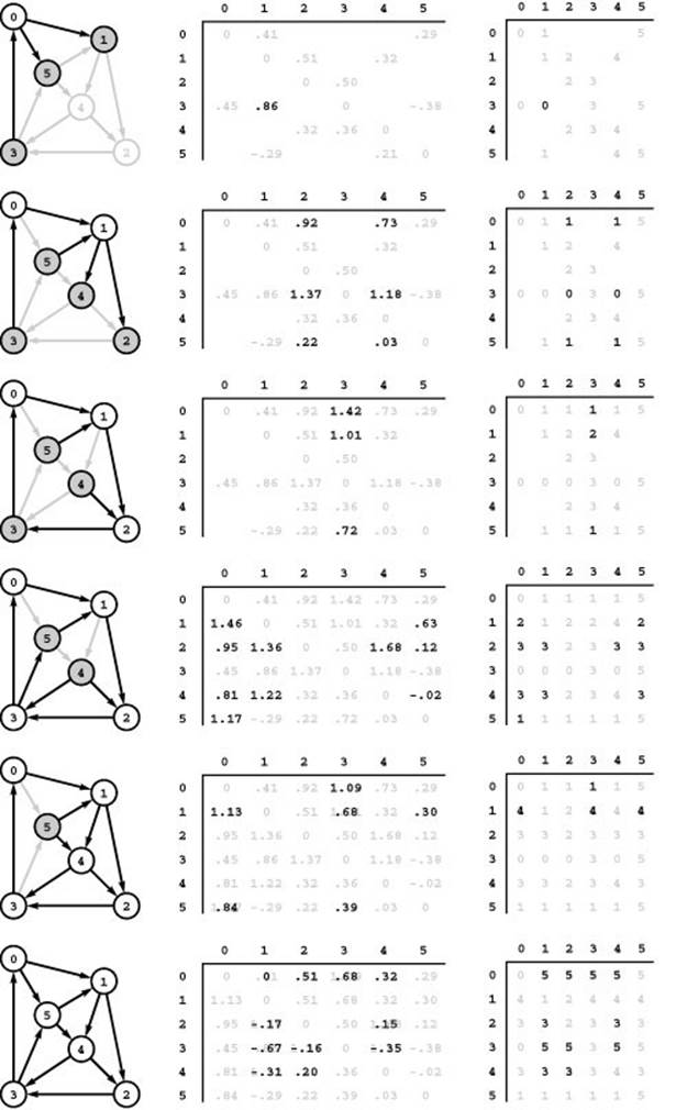
This sequence shows the construction of the all–shortest-paths matrices for a digraph with negative weights, using Floyd’s algorithm. The first step is the same as depicted in Figure 21.14. Then the negative edge 5-1 comes into play in the second step, where the paths 5-1-2 and 5-1-4 are discovered. The algorithm involves precisely the same sequence of relaxation steps for any edge weights, but the outcome differs.
wt entries to a large sentinel value, then compute shortest paths as follows:
Considering the network’s edges in any order, relax along each edge. Make V such passes.
We use the term Bellman–Ford algorithm to refer to the generic method of making V passes through the edges, considering the edges in any order. Certain authors use the term to describe a more general method (see Exercise 21.130).
For example, in a graph represented with adjacency lists, we could implement the Bellman–Ford algorithm to find the shortest paths from a start vertex s by initializing the wt entries to a value larger than any path length and the spt entries to null pointers, then proceeding as follows:
wt[s] = 0;
for (i = 0; i < G->V(); i++)
for (v = 0; v < G->V(); v++)
{
if (v != s && spt[v] == 0) continue;
typename Graph::adjIterator A(G, v);
for (Edge* e = A.beg(); !A.end(); e = A.nxt())
if (wt[e->w()] > wt[v] + e->wt())
{ wt[e->w()] = wt[v] + e->wt(); st[e->w()] = e; }
}
This code exhibits the simplicity of the basic method. It is not used in practice, however, because simple modifications yield implementations that are more efficient for most graphs, as we soon see.
Property 21.21 With the Bellman–Ford algorithm, we can solve the single-source shortest-paths problem in networks that contain no negative cycles in time proportional to V E.
Proof:We make V passes through all E edges, so the total time is proportional to V E. To show that the computation achieves the desired result, we show by induction on i that, after the ith pass, wt[v] is no greater than the length of the shortest path from s to v that contains i or fewer edges, for all vertices v. The claim is certainly true if i is 0. Assuming the claim to be true for i, there are two cases for each given vertex v: Among the paths from s to v with i+1 or fewer edges, there may or may not be a shortest path with i+1 edges. If the shortest of the paths with i+1 or fewer edges from s to v is of length i or less,
Program 21.9 Bellman–Ford algorithm
This implementation of the Bellman–Ford algorithm maintains a FIFO queue of all vertices for which relaxing along an outgoing edge could be effective. We take a vertex off the queue and relax along all of its edges. If any of them leads to a shorter path to some vertex, we put that on the queue. The sentinel value G->V separates the current batch of vertices (which changed on the last iteration) from the next batch (which change on this iteration) and allows us to stop after G->V passes.
then wt[v] will not change and will remain valid. Otherwise, there is a path from s to v with i+1 edges that is shorter than any path from s to v with i or fewer edges. That path must consist of a path with i edges from s to some vertex w plus the edge w-v. By the induction hypothesis, wt[w] is an upper bound on the shortest distance from s to w, and the (i+1)st pass checks whether each edge constitutes the final edge in a new shortest path to that edge’s destination. In particular, it checks the edge w-v.
After V-1 iterations, then, wt[v] is a lower bound on the length of any shortest path with V-1 or fewer edges from s to v, for all vertices v. We can stop after V-1 iterations because any path with V or more edges must have a (positive- or zero-cost) cycle and we could find a path with V-1 or fewer edges that is the same length or shorter by removing the cycle. Since wt[v] is the length of some path from s to v, it is also an upper bound on the shortest-path length, and therefore must be equal to the shortest-path length.
Although we did not consider it explicitly, the same proof shows that the spt vector contains pointers to the edges in the shortest-paths tree rooted at s.
For typical graphs, examining every edge on every pass is wasteful. Indeed, we can easily determine a priori that numerous edges are not going to lead to a successful relaxation in any given pass. In fact, the only edges that could lead to a change are those emanating from a vertex whose value changed on the previous pass.
Program 21.9 is a straightforward implementation where we use a FIFO queue to hold these edges so that they are the only ones examined on each pass. Figure 21.30 shows an example of this algorithm in operation.
Program 21.9 is effective for solving the single-source shortest-paths problem in networks that arise in practice, but its worst-case performance is still proportional to V E. For dense graphs, the running time is not better than for Floyd’s algorithm, which finds all shortest paths, rather than just those from a single source. For sparse graphs, the implementation of the Bellman–Ford algorithm in Program 21.9 is up to a factor of V faster than Floyd’s algorithm but is nearly a factor of V slower than the worst-case running time that we can achieve with Dijkstra’s algorithm for networks with no negative-weight edges (see Table 19.2).
Other variations of the Bellman–Ford algorithm have been studied, some of which are faster for the single-source problem than the FIFO-queue version in Program 21.9, but all take time proportional to at least V E in the worst case (see, for example, Exercise 21.132). The basic Bellman–Ford algorithm was developed decades ago; and, despite the dramatic strides in performance that we have seen for many other graph problems, we have not yet seen algorithms with better worst-case performance for networks with negative weights.
The Bellman–Ford algorithm is also a more efficient method than Floyd’s algorithm for detecting whether a network has negative cycles.
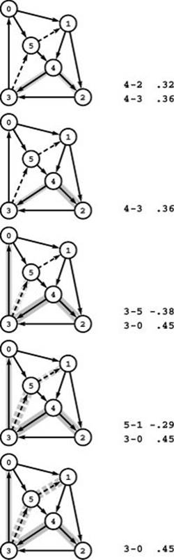
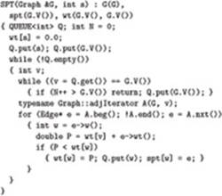
Figure 21.30 Bellman-Ford algorithm (with negative weights)
This figure shows the result of using the Bellman-Ford algorithm to find the shortest paths from vertex 4 in the network depicted in Figure Figure 21.26. The algorithm operates in passes, where we examine all edges emanating from all vertices on a FIFO queue. The contents of the queue are shown below each graph drawing, with the shaded entries representing the contents of the queue for the previous pass. When we find an edge that can reduce the length of a path from 4 to its destination, we do a relaxation operation that puts the destination vertex on the queue and the edge on the SPT. The gray edges in the graph drawings comprise the SPT after each stage, which is also shown in oriented form in the center (all edges pointing down). We begin with an empty SPT and 4 on the queue (top). In the second pass, we relax along 4-2 and 4-3, leaving 2 and 3 on the queue. In the third pass, we examine but do not relax along 2-3 and then relax along 3-0 and 3-5, leaving 0 and 5 on the queue. In the fourth pass, we relax along 5-1 and then examine but do not relax along 1-0 and 1-5, leaving 1 on the queue. In the last pass (bottom), we relax along 1-2. The algorithm initially operates like BFS, but, unlike all of our other graph search methods, it might change tree edges, as in the last step.
Property 21.22 With the Bellman–Ford algorithm, we can solve the negative-cycle–detection problem in time proportional to V E.
Proof: The basic induction in the proof of Property 21.21 is valid even in the presence of negative cycles. If we run a Vth iteration of the algorithm and any relaxation step succeeds, then we have found a shortest path with V edges that connects s to some vertex in the network. Any such path must have a cycle (connecting some vertex w to itself) and that cycle must be negative, by the inductive hypothesis, since the path from s to the second occurrence of w must be shorter than the path from s to the first occurrence of w for w to be included on the path the second time. The cycle will also be present in the tree; thus, we could also detect cycles by periodically checking the spt edges (see Exercise 21.134).
This argument holds for only those vertices that are in the same strongly connected component as the source s. To detect negative cycles in general, we can either compute the strongly connected components and initialize weights for one vertex in each component to 0 (see Exercise 21.126) or add a dummy vertex with edges to every other vertex (see Exercise 21.127).
To conclude this section, we consider the all-pairs shortest-paths problem. Can we do better than Floyd’s algorithm, which runs in time proportional to V3? Using the Bellman–Ford algorithm to solve the all-pairs problem by solving the single-source problem at each vertex exposes us to a worst-case running time that is proportional to V2E. We do not consider this solution in more detail because there is a way to guarantee that we can solve the all-paths problem in time proportional to V E log V. It is based on an idea that we considered at the beginning of this section: transforming the network into a network that has only nonnegative weights and that has the same shortest-paths structure.
In fact, we have a great deal of flexibility in transforming any network to another one with different edge weights but the same shortest paths. Suppose that a vertex-indexed vector wt contains an arbitrary assignment of weights to the vertices of a network G. With these weights, we define the operation of reweighting the graph as follows:
• To reweight an edge, add to that edge’s weight the difference between the weights of the edge’s source and destination.
• To reweight a network, reweight all of that network’s edges.
For example, the following straightforward code reweights a network, using our standard conventions:
for (v = 0; v < G->V(); v++)
{ typename Graph::adjIterator A(G, v);
for (Edge* e = A.beg(); !A.end(); e = A.nxt())
e->wt() = e->wt() + wt[v] - wt[e->w()]
}
This operation is a simple linear-time process that is well-defined for all networks, regardless of the weights. Remarkably, the shortest paths in the transformed network are the same as the shortest paths in the original network.
Property 21.23 Reweighting a network does not affect its shortest paths.
Proof: Given any two vertices s and t, reweighting changes the weight of any path from s to t, precisely by adding the difference between the weights of s and t. This fact is easy to prove by induction on the length of the path. The weight of every path from s to t is changed by the same amount when we reweight the network, long paths and short paths alike. In particular, this fact implies immediately that the shortest-path length between any two vertices in the transformed network is the same as the shortest-path length between them in the original network.
Since paths between different pairs of vertices are reweighted differently, reweighting could affect questions that involve comparing shortest-path lengths (for example, computing the network’s diameter). In such cases, we need to invert the reweighting after completing the shortest-paths computation but before using the result.
Reweighting is no help in networks with negative cycles: The operation does not change the weight of any cycle, so we cannot remove negative cycles by reweighting. But for networks with no negative cycles, we can seek to discover a set of vertex weights such that reweighting leads to edge weights that are nonnegative, no matter what the original edge weights. With nonnegative edge weights, we can then solve the all-pairs shortest-paths problem with the all-pairs version of Dijkstra’s algorithm. For example, Figure 21.31 gives such an example for our sample network, andFigure 21.32 shows the shortest-paths computation with Dijkstra’s algorithm on the transformed network with no negative edges. The following property shows that we can always find such a set of weights.
Figure 21.31 Reweighting a network
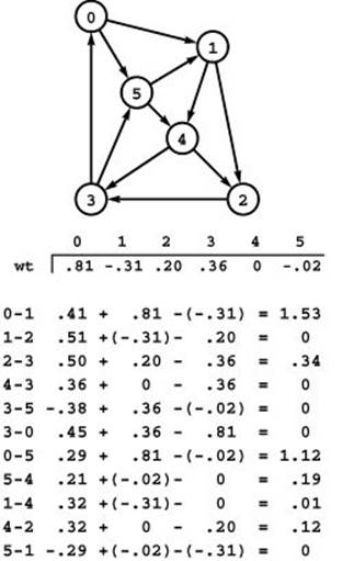
Given any assignment of weights to vertices (top), we can reweight all of the edges in a network by adding to each edge’s weight the difference of the weights of its source and destination vertices. Reweighting does not affect the shortest paths because it makes the same change to the weights of all paths connecting each pair of vertices. For example, consider the path 0-5-4-2-3: Its weight is .29 + .21 + .32 + .50 = 1.32; its weight in the reweighted network is 1.12 + .19 + .12 + .34 = 1.77; these weights differ by .45 = .81 - .36, the difference of the weights of 0 and 3; and the weights of all paths between 0 and 3 change by this same amount.
Property 21.24 In any network with no negative cycles, pick any vertex s and assign to each vertex v a weight equal to the length of a shortest path to v from s . Reweighting the network with these vertex weights yields nonnegative edge weights for each edge that connects vertices reachable from s.
Proof: Given any edge v-w, the weight of v is the length of a shortest path to v, and the weight of w is the length of a shortest path to w. If v-w is the final edge on a shortest path to w, then the difference between the weight of w and the weight of v is precisely the weight of v-w. In other words, reweighting the edge will give a weight of 0. If the shortest path through w does not go through v, then the weight of v plus the weight of v-w must be greater than or equal to the weight of w. In other words, reweighting the edge will give a positive weight.
Just as we did when we used the Bellman–Ford algorithm to detect negative cycles, we have two ways to proceed to make every edge weight nonnegative in an arbitrary network with no negative cycles. Either we can begin with a source from each strongly connected component, or we can add a dummy vertex with an edge of length 0 to every network vertex. In either case, the result is a shortest-paths spanning forest that we can use to assign weights to every vertex (weight of the path from the root to the vertex in its SPT).
For example, the weight values chosen in Figure 21.31 are precisely the lengths of shortest paths from 4, so the edges in the shortest-paths tree rooted at 4 have weight 0 in the reweighted network.
In summary, we can solve the all-pairs shortest-paths problem in networks that contain negative edge weights but no negative cycles by proceeding as follows:
• Apply the Bellman-Ford algorithm to find a shortest-paths forest in the original network.
• If the algorithm detects a negative cycle, report that fact and terminate.
• Reweight the network from the forest.
• Apply the all-pairs version of Dijkstra’s algorithm to the reweighted network.
Figure 21.32 All shortest paths in a reweighted network
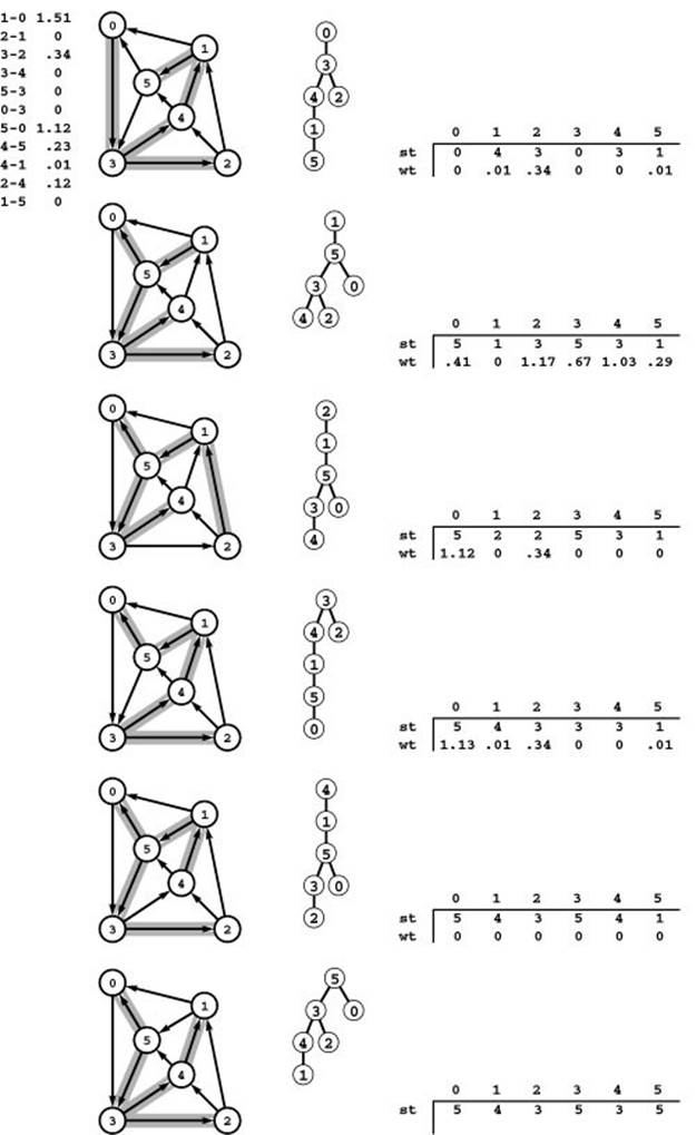
These diagrams depict the SPTs for each vertex in the reverse of the reweighted network from Figure 21.31, as could be computed with Dijkstra’s algorithm to give us shortest paths in the original network in Figure Figure 21.26. The paths are the same as for the network before reweighting, so, as in Figure 21.9, the st vectors in these diagrams are the columns of the paths matrix in Figure Figure 21.26. The wt vectors in this diagram correspond to the columns in the distances matrix, but we have to undo the reweighting for each entry by subtracting the weight of the source vertex and adding the weight of the final vertex in the path (see Figure 21.31). For example, from the third row from the bottom here we can see that the shortest path from 0 to 3 is 0-5-1-4-3 in both networks, and its length is 1.13 in the reweighted network shown here. Consulting Figure 21.31, we can calculate its length in the original network by subtracting the weight of 0 and adding the weight of 3 to get the result 1.13 - .81 + .36 = .68, the entry in row 0 and column 3 of the distances matrix in Figure Figure 21.26. All shortest paths to 4 in this network are of length 0 because we used those paths for reweighting.
After this computation, the paths matrix gives shortest paths in both networks, and the distances matrix give the path lengths in the reweighted network. This series of steps is sometimes known as John-son’s algorithm (see reference section).
Property 21.25 With Johnson’s algorithm, we can solve the all-pairs shortest-paths problem in networks that contain no negative cycles in time proportional to V E logdV, where d =2if E < 2V, and d=E/V otherwise.
Proof: See Properties 21.22 through 21.24 and the summary in the previous paragraph. The worst-case bound on the running time is immediate from Properties 21.7 and 21.22.
To implement Johnson’s algorithm, we combine the implementation of Program 21.9, the reweighting code that we gave just before Property 21.23, and the all-pairs shortest-paths implementation of Dijkstra’s algorithm in Program 21.4 (or, for dense graphs, Program 20.6). As noted in the proof of Property 21.22, we have to make appropriate modifications to the Bellman–Ford algorithm for networks that are not strongly connected (see Exercises 21.135 through 21.137). To complete the implementation of the all-pairs shortest-paths interface, we can either compute the true path lengths by subtracting the weight of the start vertex and adding the weight of the destination vertex (undoing the reweighting operation for the paths) when copying the two vectors into the distances and paths matrices in Dijkstra’s algorithm, or we can put that computation in GRAPHdist in the ADT implementation.
For networks with no negative weights, the problem of detecting cycles is easier to solve than is the problem of computing shortest paths from a single source to all other vertices; the latter problem is easier to solve than is the problem of computing shortest paths connecting all pairs of vertices. These facts match our intuition. By contrast, the analogous facts for networks that contain negative weights are counterintuitive: The algorithms that we have discussed in this section show that, for networks that have negative weights, the best known algorithms for these three problems have similar worst-case performance characteristics. For example, it is nearly as difficult, in the worst case, to determine whether a network has a single negative cycle as it is to find all shortest paths in a network of the same size that has no negative cycles.
Exercises
• 21.109 Modify your random-network generators from Exercises 21.6 and 21.7 to generate weights between a and b (where a and b are both between −1 and 1), by rescaling.
• 21.110 Modify your random-network generators from Exercises 21.6 and 21.7 to generate negative weights by negating a fixed percentage (whose value is supplied by the client) of the edge weights.
• 21.111 Develop client programs that use your generators from Exercises 21.109 and 21.110 to produce networks that have a large percentage of negative weights but have at most a few negative cycles, for as large a range of values of V and E as possible.
21.112 Find a currency-conversion table online or in a newspaper. Use it to build an arbitrage table. Note: Avoid tables that are derived (calculated) from a few values and that therefore do not give sufficiently accurate conversion information to be interesting. Extra credit: Make a killing in the money-exchange market!
• 21.113 Build a sequence of arbitrage tables using the source for conversion that you found for Exercise 21.112 (any source publishes different tables periodically). Find all the arbitrage opportunities that you can in the tables, and try to find patterns among them. For example, do opportunities persist day after day, or are they fixed quickly after they arise?
21.114 Develop a model for generating random arbitrage problems. Your goal is to generate tables that are as similar as possible to the tables that you used in Exercise 21.113.
21.115 Develop a model for generating random job-scheduling problems that include deadlines. Your goal is to generate nontrivial problems that are likely to be feasible.
21.116 Modify your interface and implementations from Exercise 21.101 to give clients the ability to pose and solve job-scheduling problems that include deadlines, using a reduction to the shortest-paths problem.
• 21.117 Explain why the following argument is invalid: The shortest-paths problem reduces to the difference-constraints problem by the construction used in the proof of Property 21.15, and the difference-constraints problem reduces trivially to linear programming, so, by Property 21.17, linear programming is NP-hard.
21.118 Does the shortest-paths problem in networks with no negative cycles reduce to the job-scheduling problem with deadlines? (Are the two problems equivalent?) Prove your answer.
• 21.119 Find the lowest-weight cycle (best arbitrage opportunity) in the example shown in Figure 21.27.
• 21.120 Prove that finding the lowest-weight cycle in a network that may have negative edge weights is NP-hard.
• 21.121 Show that Dijkstra’s algorithm does work correctly for a network in which edges that leave the source are the only edges with negative weights.
• 21.122 Develop a class based on Floyd’s algorithm that provides clients with the capability to test networks for the existence of negative cycles.
21.123 Show, in the style of Figure 21.29, the computation of all shortest paths of the network defined in Exercise 21.1, with the weights on edges 5-1 and 4-2 negated, using Floyd’s algorithm.
• 21.124 Is Floyd’s algorithm optimal for complete networks (networks with V2 edges)? Prove your answer.
21.125 Show, in the style of Figures 21.30 through 21.32, the computation of all shortest paths of the network defined in Exercise 21.1, with the weights on edges 5-1 and 4-2 negated, using the Bellman–Ford algorithm.
• 21.126 Develop a class based on the Bellman–Ford algorithm that provides clients with the capability to test networks for the existence of negative cycles, using the method of starting with a source in each strongly connected component.
• 21.127 Develop a class based on the Bellman–Ford algorithm that provides clients with the capability to test networks for the existence of negative cycles, using a dummy vertex with edges to all the network vertices.
21.128 Give a family of graphs for which Program 21.9 takes time proportional to V E to find negative cycles.
• 21.129 Show the schedule that is computed by Program 21.9 for the job-scheduling-with-deadlines problem in Exercise 21.89.
21.130 Prove that the following generic algorithm solves the single-source shortest-paths problem: “Relax any edge; continue until there are no edges that can be relaxed.”
21.131 Modify the implementation of the Bellman–Ford algorithm in Program 21.9 to use a randomized queue rather than a FIFO queue. (The result of Exercise 21.130 proves that this method is correct.)
• 21.132 Modify the implementation of the Bellman–Ford algorithm in Program 21.9 to use a deque rather than a FIFO queue such that edges are put onto the deque according to the following rule: If the edge has previously been on the deque, put it at the beginning (as in a stack); if it is being encountered for the first time, put it at the end (as in a queue).
21.133 Run empirical studies to compare the performance of the implementations in Exercises 21.131 and 21.132 with Program 21.9, for various general networks (see Exercises 21.109 through 21.111).
• 21.134 Modify the implementation of the Bellman–Ford algorithm in Program 21.9 to implement a function that returns the index of any vertex on any negative cycle or -1 if the network has no negative cycle. When a negative cycle is present, the function should also leave the spt vector such that following links in the vector in the normal way (starting with the return value) traces through the cycle.
• 21.135 Modify the implementation of the Bellman–Ford algorithm in Program 21.9 to set vertex weights as required for Johnson’s algorithm, using the following method. Each time that the queue empties, scan the spt vector to find a vertex whose weight is not yet set and rerun the algorithm with that vertex as source (to set the weights for all vertices in the same strong component as the new source), continuing until all strong components have been processed.
• 21.136 Develop an implementation of the all-pairs shortest-paths ADT interface for sparse networks (based on Johnson’s algorithm) by making appropriate modifications to Programs 21.9 and 21.4.
21.137 Develop an implementation of the all-pairs shortest-paths ADT interface for dense networks (based on Johnson’s algorithm) (see Exercises 21.136 and 21.43). Run empirical studies to compare your implementation with Floyd’s algorithm (Program 21.5), for various general networks (see Exercises 21.109 through 21.111).
• 21.138 Add a member function to your solution to Exercise 21.137 that allows a client to decrease the cost of an edge. Return a flag that indicates whether that action creates a negative cycle. If it does not, update the paths and distances matrices to reflect any new shortest paths. Your function should take time proportional to V2.
• 21.139 Extend your solution to Exercise 21.138 with member functions that allow clients to insert and delete edges.
• 21.140 Develop an algorithm that breaks the V E barrier for the single-source shortest-paths problem in general networks, for the special case where the weights are known to be bounded in absolute value by a constant.
All materials on the site are licensed Creative Commons Attribution-Sharealike 3.0 Unported CC BY-SA 3.0 & GNU Free Documentation License (GFDL)
If you are the copyright holder of any material contained on our site and intend to remove it, please contact our site administrator for approval.
© 2016-2026 All site design rights belong to S.Y.A.