Administering ArcGIS for Server (2014)

Chapter 5. Optimizing GIS Services

In the previous chapter, you learned how to analyze your requirements to plan ahead in order to move your geographic data as a service. You have acquired the skills necessary to design the GIS services into models that are ready to be deployed. With the toolset you acquired in the previous chapters, you know how to author and publish the services you design. You have learned how to consume these services from different end points. You have even written your own code to do that. Now that you've got the services up and running, it is time to manage them and make them run efficiently. After the GIS services are deployed, they usually start with a few megabytes of memory and as the consumption increases, the GIS server scoops out more and more memory for these services. Sadly, we have limited memory and processing power, so we have to distribute the GIS server's resources efficiently to those services that really need it.

In this chapter, you will learn three techniques in Server that you can apply to achieve interesting optimizing results. The first technique is pooling, where the running instances of your services are grouped in a pool. This way, each instance can be re-used several times thus serving more users. The second technique is process isolation, which helps you learn how these instances can be grouped into a single process or multiple processes to share resources. The final one you might be familiar with is caching, where the data gets stored locally on the GIS servers to save the expensive call to the database. You can control these pillars much like an equalizer to balance the efficiency of your services.

GIS service instance

Any service that you publish on ArcGIS for Server eventually gets compiled into one or more instances running on the GIS servers. They are distributed evenly throughout the GIS servers and the number of instances on each server can be configured when you publish the service. To manage these running instances in an efficient way, Esri has come up with new techniques that you will learn in the next sections.

Pooling

GIS services enabled the use of cross platforms between different environments. Now, they can be consumed by a variety of clients from different software. The classical one-to-one model of having a dedicated instance for each connection doesn't fit anymore. It was inefficient to have a new instance for every established connection; it is as if you are opening a new ArcMap document every time. The GIS services have high affinity, and they tend to consume processing and memory power rapidly, so there must be a way around it. Another model was required to be plugged into Server to manage more connections with the available limited resources. Therefore, Esri introduced the pooling technology into Server for the first time in 2007 and it was revolutionary. This model allows each connection to use a GIS service instance for a certain amount of time, which could span from milliseconds to minutes. Each instance can serve one connection at a time, for example, if one user is using ArcMap to zoom to an extent in a GIS service containing the world data, the new requested extent is sent to the Web server, which delegates the request to one of the GIS servers, which uses a free instance to execute the request. Depending on the request, the execution can take from milliseconds to minutes, and during this time the instance is labeled as busy. Once the execution is completed, the instance is released and the GIS server returns the result. This allows multiple connections to feed from one pool of instances. Using this technology, a single instance can serve up to 10 connections or even more depending on the usage.

The anatomy of pooling

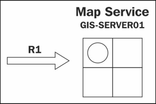
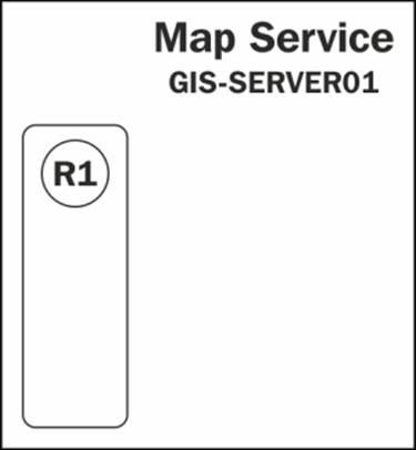
To explain pooling better, let us say that we have an electric map service running on GIS-SERVER01. You can visualize this with the following diagram. Initially, as you can see, there is one instance running:

Let's assume there is a new request R1 to zoom to a new extent to see more power cables. This request is forwarded to GIS-SERVER01 to be executed as shown in the following diagram:

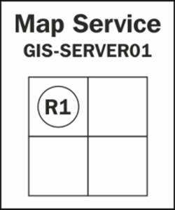
The GIS-SERVER01 finds that there is a free instance running and assigns R1 to this instance for execution as shown in the following diagram:

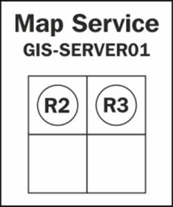
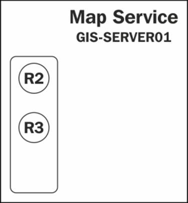
The R1 request is executed successfully. The instance is now free again for re-use. GIS-SERVER01 receives two more requests R2 and R3. They are network tracing requests, which take significantly more time to execute. There is one free instance now after executing R1and there are no other new instances available. However, there is room to create new instances so the server assigns R2 to the first instance, and creates one more instance and assigns R3 to it, as shown in the following diagram:

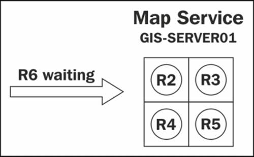
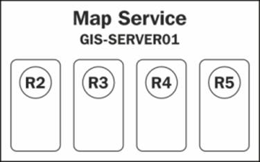
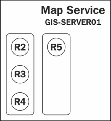
Meanwhile, three more requests come at the same time: R4 and R5, which are again tracing requests, and R6 which is a zoom-in operation. There are no available free instances, the two available instances are busy executing R2 and R3, and so the server creates two additional instances, filling up the maximum number of instances for this GIS service. Unfortunately, there is no way for Server to predict the size of the request and how long it will take so it can assign resources efficiently, but we can hope for this feature in the future releases. The worst-case scenario is that R4 and R5 get the fresh instances and R6, which is a simple zoom operation, has to wait until a free instance is available. The maximum and minimum number of instances along with the wait time can all be configured as parameters while publishing the GIS service. Refer to the following diagram:

Esri kept the pooling approach optional until Version 10.1 when it was forced as a resource management technique while publishing any service. It was kept optional because of a limitation in the pooling technology. Pooling does not remember connection history, which means a pooled connection can use different instances each time a request is initiated. This also means editing could not keep track of edit logs or web editing workflow, hence no undo or redo operations are performed. Esri managed to find a way to enable editing on pooled services starting from the 10.1 architecture.

Configuring pooled services

You will now try configuring the pooling parameters for some of the services you published in the previous chapters. These parameters should be carefully selected based on the nature of the service, for example, if a service is not used frequently, you can minimize the number of its instances. Alternatively, if a service is busy or is likely to be used more frequently, you might want to increase the number of instances. Let us take the Parcels service that you have already published. This service is considered a simple servicebecause there aren't many operations performed on Parcels. Users will only zoom and pan on Parcels features, unlike the Electricity service, where the user can run network analysis and complex operations. The Electricity service is an example of rich services. Let's try to edit the Parcels service and reconfigure the pooling parameters.

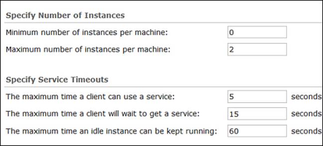
Open the ArcGIS Server Manager window and edit the Parcels service. Click on the pooling option from the list on the left-hand side. The Minimum number of instances per machine field shows the number of instances your services should start with. Currently it is 1, which means a single instance will run whenever you activate this service. Also note that it says "per machine", which means that this will be applied to each GIS server. So if I have two GIS servers, GIS-SERVER01 and GIS-SERVER02 configured on my Server site, I will have a single instance running on each server, which makes a total of two instances. Setting Minimum number of instances per machine to 2 will result in four instances. If I know that Parcels data are rarely queried in this context, meaning there is no need for it to occupy an instance at startup, I would change this parameter to 0. Don't worry! Whenever someone requests the Parcels service, a new instance will be created and the request will be fulfilled. Go ahead and set the minimum instances to 0. The second parameter is Maximum number of instances per machine. This field sets the threshold to the number of instances in a GIS service. Users of the service have to wait for a free instance if the maximum numbers of instances are all in use and no new instances will be created. You can set this parameter to 1, since there are no complex operations on the Parcels service and one instance can serve plenty of users. While the instance is busy serving a request, other users have to wait. Now, this wait time can also be configured in the The maximum time a client will wait to get a service field. It is currently set to a minute, which is quite a long time. It is better to reduce this time because we know that a zoom-in, zoom-out, or pan operation shouldn't take more than few seconds in worst cases. So change this parameter to 15 seconds. Any request that takes more than 15 seconds to be fulfilled should be discarded and requested again. This way we save more memory at the buffer at a slight cost of unsatisfying a few requests. Similarly, the field The maximum time a client can use a service is used to configure how long a client can consume an instance. We know that all operations on Parcels are simple and shouldn't take more than 5 seconds. Currently, it is set by default at 600 seconds, which is an average figure Esri came up with. The default value might be different depending on the version of Server. If a request takes more than that, it means something went wrong, perhaps a network failure, an infinite logic loop, and so on. Server can terminate the request and free the instance for other healthier requests. Any service that is not used for a long time should be removed from the memory to free up space for other services.

We could argue over what a long time really is, but in our example, Parcels are rarely queried and they consume a lot of memory due to their size. So instead of 30 minutes, I would set the The maximum time an idle instance can be kept running to 1 minute (60seconds) as shown in the following screenshot:

Tip

Best practice

Determine whether your service is simple or rich before configuration as this will help you set optimal pooling parameters.

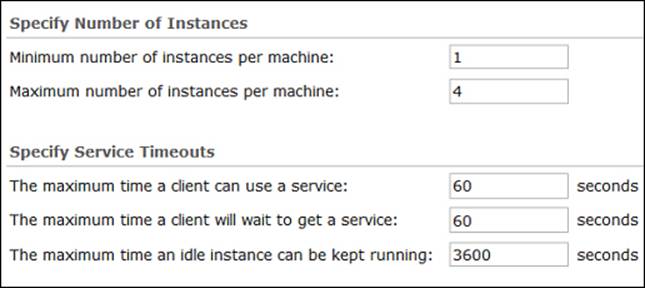
Let us modify the pooling configuration for the Electricity service. Note that this service is more vital as we have called it a typical request that can take a significant amount of time to execute. It is not just a zoom operation, it could be tracing, network analysis, and many complex operations, therefore instances should be available at all times. As you can see in the following screenshot, I have increased the minimum and maximum instances. There must be at least one instance running and enough room for more instances. I have also increased the idle time to one hour, so even if the instance is idle, it should stay for an hour before it gets removed. We did that because it is expensive to create an instance. It takes time and we want to fulfill requests to this service in a responsive manner. The following screenshot shows the configuration we selected for the Electricity service:

Tip

Best practice

Never use the default pooling parameters on a production setup. Always analyze the nature of your services and carefully set the pooling parameters accordingly.

Process isolation

Process isolation is another optimization technique that controls the number of GIS-service instances in a process. You can either perform high or low process isolation and each has its merits. By having more instances in a single process, you are performing a low-isolation technique. By lowering the number of instances, you are spreading your instances into multiple processes, thus performing a higher isolation. In Server, having a single instance in a process is referred to as high isolation.

High-isolation configuration

By isolating each instance in a single process the instance will have its own dedicated area in the memory heap. This means a service with high isolation is less likely to experience downtime and failure. Even if a process is terminated or a memory leakage happened in one of the processes, only one instance will be recycled while the rest of the instances will remain available. Since each instance requires a dedicated process in this approach, this will require more memory, thus your GIS server should have more RAM to accommodate such configuration.

Note

Services with high isolation techniques are more stable, but they require more memory because each instance in a service reserves its own process.

Let us revisit the same example we used in the pooling topic, this time with high isolation configuration. Initially, the Electricity GIS service has one minimum instance running, which means in this configuration one process should be running. In the following diagram, the rounded rectangle is the process and the circle is the instance. Request R1 comes and there is a free instance, so it is assigned to it for execution:

Request R1 is completed and the instance is now free again for re-use. For requests R2 and R3, there is one free instance now after executing R1 and there are no other new instances available, so GIS-SERVER01 creates a new process to host a new instance as shown in the following diagram:

Meanwhile, R4, R5, and R6 are received while the server is busy executing R2 and R3. There are not enough instances, and so the server creates two more processes for the new requests. The R6 request has to wait for a free instance because according to the pooling configuration there is a maximum of four instances per server, as shown in the following diagram:

Low-isolation configuration

Low isolation configuration requires less memory as it groups multiple instances in a single process. These instances share the same allocated memory with their siblings in the same process. The downside of this approach is that when a process fails, all instances hosted by this process are withered.

Note

Services with low isolation techniques require less memory but they are more likely to become unavailable in the event of a process failure.

Let's see how a service with low isolation configuration of three instances per process behaves. The request R1 is received; there is a free instance to which it is assigned:

Request R1 is completed, R2 and R3 are received, R2 is assigned the free instance, and R3 has to have a new instance. The new instance is created in the same process, as shown in the following diagram:

While the server is busy executing R2 and R3, the requests R4, R5, and R6 are received. A new instance is created for R4. This fills out the first process and the server has to create a new process to host the new requests. The second process is created with a new instance to which R5 is assigned. Again, R6 has to wait since we are allowed to have a maximum of four instances. Notice that we have consumed less memory with this configuration. Refer to the following diagram:

Configuring process isolation

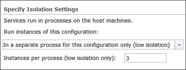
Now that we know how the process isolation works, we need to learn how to configure it. Edit one of your services from the ArcGIS Server Manager window and click on the Processes tab. From Specify Isolation Settings, select Low Isolation or High Isolationdepending on your preferences. If you however selected Low Isolation, you will notice that you can change the number of the Instances per process field, as shown in the following screenshot:

Recycling and health check

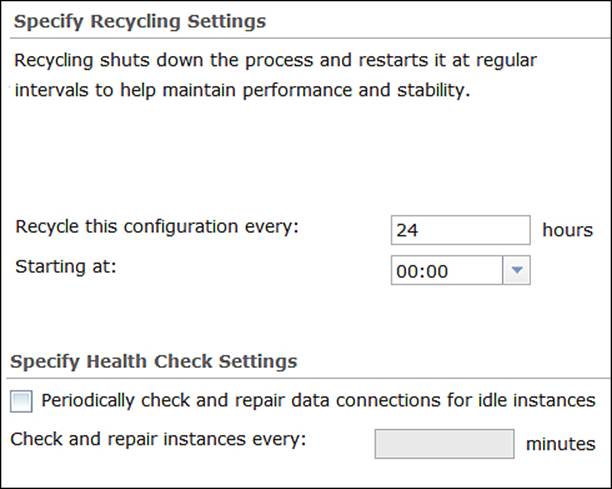
The operating system periodically runs diagnostics and analysis on the memory and does some modification on the data address such as defragmentation and other routine tasks to optimize the running processes. However, the OS does not maintain the internal part of an allocated memory, therefore, ArcGIS for Server provides you with the option to recycle process isolation configuration periodically so that the OS routine optimizing tasks can kick-in to help maintain performance and stability. You can change Recycling Interval from the Processes tab to recycle. Server also provides the option Periodically check and repair data connections for idle instances. It allows Server to periodically scan for idle instances and verify that they can still connect successfully to the database. I usually uncheck this option as it adds an extra cost on the GIS servers. The pooling configurations we specified earlier are enough to clear idle instances. If you do want to enable this option, make sure that this interval spans wide, over an hour, to avoid making unnecessary connections to the database. The following is the screenshot of the recycling configurations:

Tip

Best practice

It is more efficient to shut down an instance with idle connections instead of repairing it.

Caching

Caching is probably the most effective optimization tool to speed up the services' response time. When executing a particular request, the GIS server spends almost all of the execution time connecting to the database, indexing, querying, retrieving records, geoprocessing, projecting, and writing the map to an image, which is finally returned. You may notice that all these operations are database related. So if you could eliminate the database factor, you could save a huge amount of processing time. Here is where the concept of caching is introduced. If you could generate tiles of images for certain scales and store them locally on the GIS server's physical hard drive, you can simply index a request to a set of tiles and return them immediately without connecting to the database and doing all this overhead work. Caching could slash a big portion of processing time, minimizing the response time to more than 80 percent and consequently increasing successful requests or throughput. Not only can this optimize the service-request processing, it can also minimize the number of queries to the database to make it healthier and more responsive to other high priority queries. Caching doesn't come without flaws though. Saving images of different scales for different layers requires, well, storage. To do a good caching that is noticeable, you need at least 10 to 20 gigabytes of free disk space depending on the size of your database, and that is a lot. Moreover, if your data is frequently edited, you might not get much out of caching since your users will see an older version of the data, a cached version. Unless you update the cache frequently you will end up with an outdated service that is fast to load, but not very useful.

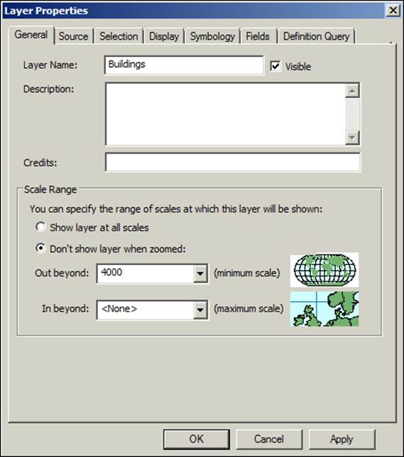
We will now create caching for the Building service. We don't have this service on our Server site yet, but we will author and publish it. Let us assume that you get the Buildings data on CDs on a yearly basis, where you then move them into your database. In this case, you can safely cache this data and use it for a year before you update it. It is efficient to create the Building cache to save database hits and speed up the loading process. Open ArcMap and browse to the Building feature class in7364EN_05_Codes\AGSA\Data\Buildings.gdb and add it to the map. Change the symbology to the BuildingType category so that we can differentiate the types of buildings. We have done that previously so it should be an easy task. Now, we have to set the scale on which the building layer is visible. We will set the minimum scale to 1:4000; this means zooming out beyond 4000—any scale number larger than 4000—will render the building invisible.

To do that, double-click on the Building layer from the table of content and activate the General tab. Select Don't show layer when zoomed, type 4000 in the Out beyond field, and click on OK, as shown in the following screenshot:

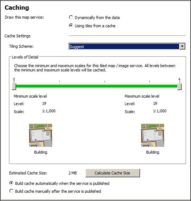
Go ahead and publish your new building document as a service. Refer to Chapter 2, Authoring Web Services, for detailed steps. From the Service Editor window, activate the Caching tab from the left-hand side and then select Using tiles from a cache to enable caching. The tiling scheme is the theme by which you want to cache your service. You can mimic an existing service such as Google Maps or you can create your own. Since we do not have any cached service, we will let Server suggest the tile scheme for us. Select Suggest from the Tiling Scheme drop-down list as shown in the following screenshot:

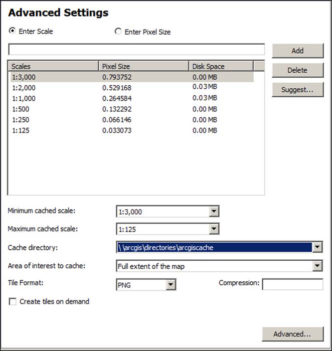
Open the Advanced Settings window. You will see that Server suggested four scale levels starting from 1000 going down to 125. We need to add two more scale levels 2000 and 3000 and use the Add button to add the two scale levels. Note that Server calculates the disk space necessary for each scale level as well. Don't forget to register your database before you click on Publish. The following screenshot illustrates the different scale levels:

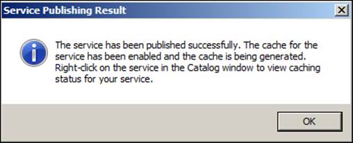
After publishing is completed, you will see a message indicating that your service has been published; however, the caching is still building. Caching is a long process and it requires sometime. GIS servers will be busy during caching so it is recommended that you do it during less busy hours. The screenshot for the Service Publishing Result message prompt is as follows:

Another approach to building the cache for a service is through the geoprocessing tools. Although you can create and manage your cache from the ArcGIS for Server Manager window, I would advise you to do it from ArcCatalog, the reason being that caching takes a huge amount of time and consumes almost the entire memory. ArcGIS for Server Manager is a web interface, which runs on a browser unlike ArcCatalog, which is a standalone executable program that can withhold heavy operation. Start ArcCatalog and create an administrator connection to your Server site. Here is how you create an admin connection:

1. From Catalog Tree, expand the GIS Servers node.

2. Double-click on the Add ArcGIS Server node to add a new connection.

3. From the Add ArcGIS Server form, select Administer GIS Server and then click on Next.

4. In the Server URL, type in your server site address: http://GIS-SERVER01:6080/arcgis.

5. Type in the primary administrator Username and Password and click on Finish.

6. Rename the connection to Admin@GIS-SERVER01.

Activate the connection; you will see the list of all your services. Now, we need to open ArcToolbox and run the geoprocessing tool that will create the cache for us. From ArcToolBox, expand the Server Tools and Caching nodes to see the list of caching tools we have. Double-click on the Create Map Service Cache tool:

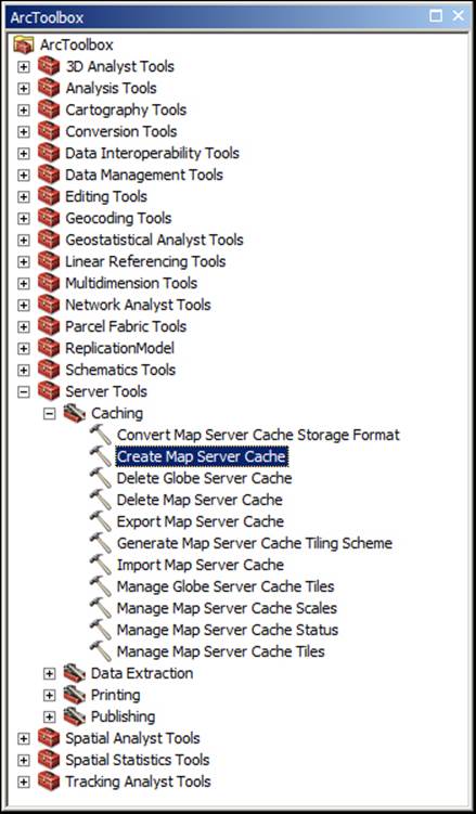
A new window will pop up. You will experience a similar look and feel when working with geoprocessing forms. Esri adopted the concept of model builders in the previous few releases of ArcGIS, and it is clearly planning to move its core functionality into geoprocessing tools. With this, users can re-use and mash these tools together to build bigger models. In the Create Map Server Cache form, you need to select the Input Service option you want to cache. You can use the Browse button or conveniently drag it from the catalog tree to the input box. The Service Cache Directory dialog box will be automatically populated. If you remember, you already configured that in the Server site back in Chapter 1, Best Practices for Installing ArcGIS for Server, ArcGIS for Server populates it for you. This folder is basically the output of the caching operation where the cache is stored. Next are the scales. It is not feasible to create cache for all scales as this will require unlimited space. Cache has to be created for certain scales: the busy scales which are asked for frequently. Server helps you analyze your service and recommend certain scales to cache, for example, it is pointless to cache scales on which layers are invisible. Select New for Tiling Scheme and Standard for Scale Type, and in theNumber of Scales field type 3. Server will suggest three different scales. Leave the rest of the options to default and click on OK. You should see the following prompt message when the tool finished running:

If you are planning to cache more services, it might be a good idea to create your own template tiling scheme and then apply it on the new service. In this template, there is an XML file that contains the default scales, image Dot per Inch (DPI), compression, tile size, and other parameters. You can generate the tiling scheme file using the Generate Tile Cache Tiling Scheme tool from ArcToolBox. Then you can use the XML tile scheme to enable caching from the Server Editor while creating or editing the service.

Tip

Best practice

Planning the scales you want to cache is crucial. You have to see at what scales your service gets busy, and cache those scales accordingly.

Summary

If there was unlimited memory and processing power, you wouldn't have to optimize your GIS services and I wouldn't have written this chapter. However, unfortunately, we do have limited resources and we have to use them efficiently to get our services to run comfortably. In this chapter, you have learned a number of approaches to optimize your ArcGIS for Server. You now know that careful planning and analysis is required to select the correct parameters and preferences that will make your Server run at its optimal state. The techniques you learned, namely pooling, process isolation, and caching are sufficient, if used as guided, to bring the most out of your ArcGIS for Server and make your GIS services run much more efficiently and effectively. In the next chapter, you will be introduced to the clustering technique. This will help you group and categorize your GIS servers in order to use them more effectively.