Learning Ceph (2015)

Chapter 10. Ceph Performance Tuning and Benchmarking

In this chapter, we will cover the following topics:

· Ceph performance overview

· General Ceph performance consideration – hardware level

· Ceph performance tuning – software level

· Ceph erasure coding

· Ceph cache tiering

· Ceph benchmarking using RADOS bench

Ceph performance overview

Data and information always keep on changing and increasing. Every organization, whether small or large, faces data growth challenges with time, and most of the time, these data growth challenges bring performance problems with them. In this era, where the world is generating enormous amount of data, organizations have to look for a storage solution that is highly scalable, distributed, extremely reliable, and on top of that, well performing for all of their workload needs.

One of the several biggest advantages of Ceph is that it possesses scalable, distributed architecture. Due to its distributed nature, all the workload that comes to Ceph is evenly distributed and allocated to the entire cluster for storage, which makes Ceph a good performing storage system. You can imagine storing a data file on a traditional storage system is quite limited in scalability, almost nondistributed, and has only a limited numbers of data storage nodes and disks. In such a kind of traditional setup, performance problems might occur with data growth and increasing user requests.

These days, when applications serve a huge number of clients, they require a better-performing backend storage system. A typical Ceph setup contains numerous nodes, and each node contains several OSDs. Since Ceph is distributed, when data arrives to Ceph for storage, it's distributed across several nodes and OSDs beneath, delivering an accumulative performance of several nodes. Moreover, the traditional systems are limited to a certain performance when you add more capacity to them, that is, you will not get added performance with increasing capacity. In some scenarios, the performance degrades on increasing the capacity. With Ceph, you will never see performance degradation with increase in the capacity. When you increase the capacity of a Ceph storage system, that is, when you add new nodes full of OSDs, the performance of the entire storage cluster increases linearly since we now get more OSD workhorses and added CPU, memory, and network per new node. This is something that makes Ceph unique and differentiates Ceph from other storage systems.

Ceph performance consideration – hardware level

When it comes to performance, the underlying hardware plays a major role. Traditional storage systems run specifically on their vendor-manufactured hardware, where users do not have any flexibility in terms of hardware selection based on their needs and unique workload requirements. It's very difficult for organizations that invest in such vendor-locked systems to overcome problems generated due to incapable hardware.

Ceph, on the other hand, is absolutely vendor-free; organizations are no longer tied up with hardware manufacturers, and they are free to use any hardware of their choice, budget, and performance requirements. They have full control over their hardware and the underlying infrastructure.

The other advantage of Ceph is that it supports heterogeneous hardware, that is, Ceph can run on cluster hardware from multiple vendors. Customers are allowed to mix hardware brands while creating their Ceph infrastructure. For example, while purchasing hardware for Ceph, customers can mix the hardware from different manufacturers such as HP, Dell, IBM, Fujitsu, Super Micro, and even off-the-shelf hardware. In this way, customers can achieve huge money-savings, their desired hardware, full control, and decision-making rights.

Hardware selection plays a vital role in the overall Ceph storage performance. Since the customers have full rights to select the hardware type for Ceph, it should be done with extra care, with proper estimation of the current and future workloads.

One should keep in mind that hardware selection for Ceph is totally dependent on the workload that you will put on your cluster, the environment, and all features you will use. In this section, we will learn some general practices for selecting hardware for your Ceph cluster.

Processor

Some of the Ceph components are not processor hungry. Like Ceph, monitor daemons are lightweight, as they maintain copies of cluster and do not serve any data to clients. Thus, for most cases, a single core processor for monitor will do the job. You can also think of running monitor daemons on any other server in your environment that has free resources. Make sure you have system resources such as memory, network, and disk space available in an adequate quantity for monitor daemons.

Ceph OSD daemons might require a fair amount of CPU as they serve data to clients and hence require some data processing. A dual-core processor for OSD nodes will be nice. From a performance point of view, it's important to know how you will use OSDs, whether it's in a replicated fashion or erasure coded. If you use OSDs in erasure coding, you should consider a quad-core processor as erasure-coding operations require a lot of computation. In the event of cluster recovery, the processor consumption by OSD daemons increases significantly.

Ceph MDS daemons are more process hungry as compared to MON and OSD. They need to dynamically redistribute their load that is CPU intensive; you should consider a quad-core processor for Ceph MDS.

Memory

Monitor and metadata daemons need to serve their data rapidly, hence they should have enough memory for faster processing. From a performance point of view, 2 GB or more per-daemon instance should be available for metadata and monitor. OSDs are generally not memory intensive. For an average workload, 1 GB of memory per-OSD-daemon instance should suffice; however, from a performance point of view, 2 GB per-OSD daemon will be a good choice. This recommendation assumes that you are using one OSD daemon for one physical disk. If you use more than one physical disk per OSD, your memory requirement will grow as well. Generally, more physical memory is good, since during cluster recovery, memory consumption increases significantly.

Network

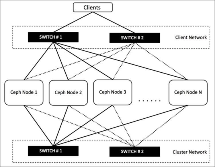
All the cluster nodes should have dual-network interfaces for two different networks, that is, cluster network and client network. For a medium-size cluster of several hundred terabytes, 1 G network link should go well. However, if your cluster size is big and it serves several clients, you should think of 10 G or more bandwidth network. At the time of system recovery, network plays a vital role. If you have a good 10 G or more bandwidth network connection, your cluster will recover quickly, else it might take some time. So, from a performance point of view, 10 Gb or more dual network will be a good option. A well-designed Ceph cluster makes use of two physically separated networks, one for cluster network (internal network) and another for client network (external network); both these networks should be physically separated from the network switch; a point-of-availability setup will require a redundant dual network, as shown in the following diagram:

Disk

Disk drive selection for Ceph storage cluster holds a lot of importance with respect to overall performance and the total cluster cost. Before taking your final decision on disk drive selection, you should understand your workload and possible performance requirements. Ceph OSD consists of two different parts: the OSD journal part and the OSD data part. Every write operation is a two-step process.

When any OSD receives client requests to store an object, it first writes the object to the journal part, and then from the journal, it writes the same object to the data part before it sends an acknowledge signal to the client. In this way, all the cluster performance revolves around OSD journal and data partition. From a performance point of view, it's recommended to use SSD for journals. By using SSD, you can achieve significant throughput improvements by reducing access time and read latency. In most environments, where you are not concerned about extreme performance, you can consider configuring journal and data partition on the same hard disk drive. However, if you are looking for significant performance improvements out of your Ceph cluster, it's worth investing on SSD for journals.

To use SSD as journals, we create logical partitions on each physical SSD that will be used as journals, such that each SSD journal partition is mapped to one OSD data partition. In this type of setup, you should keep in mind not to overload SSDs by storing multiple journals beyond its limits. By doing this, you will impact the overall performance. To achieve good performance out of your SSDs, you should store no more than four OSD journals on each SSD disk.

The dark side of using a single SSD for multiple journals is that if you lose your SSD hosting multiple journals, all the OSDs associated with this SSD will fail and you might lose your data. However, you can overcome this situation by using RAID 1 for journals, but this will increase your storage cost. Also, SSD cost per gigabyte is nearly 10 times more compared to HDD. So, if you are building a cluster with SSDs, it will increase the cost per gigabyte for your Ceph cluster.

Filesystem type selection is also one of the aspects for cluster performance. Btrfs is an advance filesystem that can write the object in a single operation as compared to XFS and EXT4, which require two steps to write an object. Btrfs is copy-on-write filesystem, that is, while writing the object to journal, it can simultaneously write the same object on data partition, providing significant performance improvements. However, Btrfs is not production ready at the time of writing. You might face data inconsistency problems with Btrfs.

Ceph performance tuning – software level

The performance of any system is quantified by load and performance testing. The results of these tests help us to make the decision whether the current setup requires tuning or not. Performance tuning is the process of rectifying performance bottlenecks identified during performance tests. Performance tuning is a very vast topic, which requires a deep study of each and every component, whether it's internal or external to Ceph.

The recommended approach to fine-tune a Ceph cluster is to start investigation from one end of the cluster's smallest element up to the level of end users who use the storage services. In this section, we will cover some performance tuning parameters from a Ceph cluster's point of view. We will define these performance tuning parameters under a Ceph cluster configuration file so that each time any Ceph daemon starts, it should adhere to the tuning setting. We will first learn about Ceph configuration files and its various sections, and then we will focus on performance tuning settings.

Cluster configuration file

Most of the cluster-wide configuration settings are defined under a Ceph cluster configuration file. If you have not changed your cluster name and configuration file location for your cluster, the default name will be ceph.conf and the path will be /etc/ceph/ceph.conf. This configuration file has a global section as well as several sections for each service type. Whenever each Ceph service type starts, that is, MON, OSD, and MDS, it reads the configuration defined under the global section as well as their specific section.

Config sections

A Ceph configuration file has multiple sections; we will now discuss the role of each section of configuration file.

The global section

The global section is the section defined under [global]; all the settings under this section affect all the daemons of a Ceph cluster. The setting that needs to be applied for the entire cluster is defined here. The following is the example of the settings in this section:

public network = 192.168.0.0/24

The MON section

The settings mentioned under the [MON] section are applied to all ceph-mon daemons in the Ceph cluster. The configuration defined under this section overrides the same settings defined under the [global] section. The following is the example of the settings in this section:

mon initial members = ceph-mon1

The OSD section

The settings mentioned under the [OSD] section are applied to all ceph-osd daemons in the Ceph cluster. The configuration defined under this section overrides the same setting defined under the [global] section. The following is the example of the settings in this section:

osd mkfs type = xfs

The MDS section

The settings mentioned under the [MDS] section are applied to all ceph-mds daemons in the Ceph cluster. The configuration defined under this section overrides the same setting defined under the [global] section. The following is the example of the settings in this section:

mds cache size = 250000

The client section

The settings mentioned under the [client] section are applied to all Ceph clients. The configuration defined under this section overrides the same setting defined under the [global] section. The following is the example of the settings in this section:

rbd cache = true

Ceph cluster performance tuning

As mentioned earlier, performance tuning is mostly environment-specific. Your organization environment and hardware infrastructure for Ceph cluster will be a lot different from other organizations. Things you tune for your Ceph cluster may or may not work the same way as in other environments. In this section, we will discuss some general performance tuning parameters that you can tailor more specifically for your environment.

Global tuning parameters

The parameters mentioned in this section should be defined under the [global] section of your Ceph cluster configuration file.

Network

It's highly recommended that you use two physically separated networks for your Ceph cluster. Each of these networks has their own set of responsibilities. Under Ceph's terminology, these networks are referred to as public and cluster networks:

· The public network is also referred to as the client-side network that allows clients to communicate with Ceph clusters and access the cluster for their data storage. This network is dedicated to clients only, so no internal cluster communication happens on this network. You should define the public network for your Ceph cluster configuration as follows:

public network = {public network / netmask}

The example of this will be as follows:

public network = 192.168.100.0/24

· The cluster network is also referred to as the internal network, which is a dedicated network for all the internal cluster operations between Ceph nodes. From a performance point of view, this network should have a decent bandwidth of 10 Gb or 40 Gb as this network is responsible for high bandwidth cluster operations such as data replication, recovery, rebalancing, and heartbeat checks. You can define cluster network as follows:

cluster network = {cluster network / netmask}

The example of this will be as follows:

cluster network = 192.168.1.0/24

Max open files

If this parameter is in place and the Ceph cluster starts, it sets the max open file descriptors at the OS level. This helps OSD daemons from running out of file descriptors. The default vale of this parameter is 0; you can set it as up to a 64-bit integer.

Have a look at the following example:

max open files = 131072

OSD tuning parameters

The parameters mentioned in this section should be defined under the [OSD] section of your Ceph cluster configuration file:

· Extended attributes: These are also known as XATTRs, which are very valuable for storing file metadata. Some filesystems allow a limited set of bytes to store as XATTRs. In some cases, using well-defined extended attributes will help the filesystem. The XATTR parameters should be used with an EXT4 filesystem to achieve good performance. The following is the example:

filestore xattr use omap = true

· Filestore sync interval: In order to create a consistent commit point, the filestore needs to quiesce write operations and do a syncfs, which syncs data from the journal to the data partition, and thus frees the journal. A more frequent sync operation reduces the amount of data that is stored in a journal. In such cases, the journal becomes underutilized. Configuring less frequent syncs allows the filesystem to coalesce small writes better, and we might get an improved performance. The following parameters define the minimum and maximum time period between two syncs:

· filestore min sync interval = 10

filestore max sync interval = 15

Note

You can set any other double-type value that better suits your environment for filestore min and filestore max.

· Filestore queue: The following settings allow a limit on the size of a filestore queue. These settings might have minimal impact on performance:

· filestore queue max ops: This is the maximum number of operations that a filestore can accept before blocking new operations to join the queue. Have a look at the following example:

filestore queue max ops = 25000

· filestore queue max bytes: This is the maximum number of bytes of an operation. The following is the example:

filestore queue max bytes = 10485760

· filestore queue committing max ops: This is the maximum number of operations the filestores can commit. An example for this is as follows:

filestore queue committing max ops = 5000

· filestore queue committing max bytes: This is the maximum number of bytes the filestore can commit. Have a look at the following example:

filestore queue committing max bytes = 10485760000

· filestore op threads: This is the number of filesystem operation threads that can execute in parallel. The following is the example:

filestore op threads = 32

· OSD journal tuning: Ceph OSD daemons support the following journal configurations:

· journal max write bytes: This is the maximum number of bytes the journal can write at once. The following is the example:

journal max write bytes = 1073714824

· journal max write entries: This is the maximum number of entries the journal can write at once. Here is the example:

journal max write entries = 10000

· journal queue max ops: This is the maximum number of operations allowed in the journal queue at one time. An example of this is as follows:

journal queue max ops = 50000

· journal queue max bytes: This is the maximum number of bytes allowed in the journal queue at one time. Have a look at the following example:

journal queue max bytes = 10485760000

· OSD config tuning: Ceph OSD daemons support the following OSD config settings:

· osd max write size: This is the maximum size in megabytes an OSD can write at a time. The following is the example:

osd max write size = 512

· osd client message size cap: This is the maximum size of client data in megabytes that is allowed in memory. An example is as follows:

osd client message size cap = 2048

· osd deep scrub stride: This is the size in bytes that is read by OSDs when doing a deep scrub. Have a look at the following example:

osd deep scrub stride = 131072

· osd op threads: This is the number of operation threads used by a Ceph OSD daemon. For example:

osd op threads = 16

· osd disk threads: This is the number of disk threads to perform OSD-intensive operations such as recovery and scrubbing. The following is the example:

osd disk threads = 4

· osd map cache size: This is the size of OSD map cache in megabytes. The following is the example:

osd map cache size = 1024

· osd map cache bl size: This is the size of OSD map caches stored in-memory in megabytes. An example is as follows:

osd map cache bl size = 128

· osd mount options xfs: This allows us to supply xfs filesystem mount options. At the time of mounting OSDs, it will get mounted with supplied mount options. Have a look at the following example:

osd mount options xfs = "rw,noatime,inode64,logbsize=256k,delaylog,allocsize=4M"

· OSD recovery tuning: These settings should be used when you like performance over recovery or vice versa. If your Ceph cluster is unhealthy and is under recovery, you might not get its usual performance as OSDs will be busy into recovery. If you still prefer performance over recovery, you can reduce recovery priority to keep OSDs less occupied with recovery. You can also set these values if you want a quick recovery for your cluster, helping OSDs to perform recovery faster.

· osd recovery op priority: This is the priority set for recovery operation. Lower the number, higher the recovery priority. Higher recovery priority might cause performance degradation until recovery completes. The following is the example:

osd recovery op priority = 4

· osd recovery max active: This is the maximum number of active recover requests. Higher the number, quicker the recovery, which might impact the overall cluster performance until recovery finishes. The following is the example:

osd recovery max active = 10

· osd max backfills: This is the maximum number of backfill operations allowed to/from OSD. The higher the number, the quicker the recovery, which might impact overall cluster performance until recovery finishes. The following is the example:

osd recovery max backfills = 4

Client tuning parameters

The user space implementation of a Ceph block device cannot take advantage of a Linux page cache, so a new in-memory caching mechanism has been introduced in Ceph Version 0.46, which is known as RBD Caching. By default, Ceph does not allow RBD caching; to enable this feature, you should update the [client] section of your Ceph cluster configuration file with the following parameters:

· rbd cache = true: This is to enable RBD caching.

· rbd cache size = 268435456: This is the RBD cache size in bytes.

· rbd cache max dirty = 134217728: This is the dirty limit in bytes; after this specified limit, data will be flushed to the backing store. If this value is set to 0, Ceph uses the write-through caching method. If this parameter is not used, the default cache mechanism is write-back.

· rbd cache max dirty age = 5: This is the number of seconds during which dirty data will be stored on cache before it's flushed to the backing store.

General performance tuning

In the last section, we covered various tuning parameters that you can define under your cluster configuration file. These were absolute Ceph-based tuning tips. In this section, we will learn a few general tuning tips, which will be configured at OS- and network-level for your infrastructure:

· Kernel pid max: This is a Linux kernel parameter that is responsible for maximum number of threads and process IDs. A major part of the Linux kernel has a relatively small kernel.pid_max value. Configuring this parameter with a higher value on Ceph nodes having greater number of OSDs, that is, OSD > 20, might help spawning multiple threads for faster recovery and rebalancing. To use this parameter, execute the following command from the root user:

· # echo 4194303 > /proc/sys/kernel/pid_max

· Jumbo frames: The Ethernet frames that are more than 1,500 bytes of payload MTU are known as jumbo frames. Enabling jumbo frames of all the network interfaces of your Ceph cluster node should provide better network throughput and overall improved performance. The jumbo frames are configured at an OS level, however, the network interface and backend network switch should support jumbo frames. To enable jumbo frames, you should configure your switch-side interfaces to accept them and then start configuring at the OS level. For instance, from an OS point of view, to enable jumbo frames on interface eth0, execute the following command:

· # ifconfig eth0 mtu 9000

9,000 bytes of payload is the maximum limit of network interface MTU; you should also update your network interface configuration file, /etc/sysconfig/network-script/ifcfg-eth0, to MTU=9000, in order to make the change permanent.

· Disk read_ahead: The read_ahead parameter speeds up the disk read operation by prefetching data and loading it to random access memory. Setting up a relatively higher value for read_ahead will benefit clients performing sequential read operations. You can check the current read_ahead value using this command:

· # cat /sys/block/vda/queue/read_ahead_kb

To set read_ahead to a higher value, execute the following command:

# echo "8192">/sys/block/vda/queue/read_ahead_kb

Typically, customized read_ahead settings are used on Ceph clients that use RBD. You should change read_ahead for all the RBDs mapped to this host; also make sure to use the correct device path name.

Ceph erasure coding

Data protection and redundancy technologies have existed for many decades. One of the most popular methods for data reliability is replication. The replication method involves storing the same data multiple times on different physical locations. This method proves to be good when it comes to performance and data reliability, but it increases the overall cost associated with a storage system. The TOC with a replication method is way too high.

This method requires double the amount of storage space to provide redundancy. For instance, if you are planning for a storage solution with 1 PB of data with a replication factor of one, you will require a 2 PB of physical storage to store 1 PB of replicated data. In this way, the replication cost per gigabyte of storage system increases significantly. You might ignore the storage cost for a small storage cluster, but imagine where the cost will hit if you build up a hyper-scale data storage solution based on replicated storage backend.

Erasure coding mechanism comes as a gift in such scenarios. It is the mechanism used in storage for data protection and data reliability, which is absolutely different from the replication method. It guarantees data protection by dividing each storage object into smaller chunks known as data chunks, expanding and encoding them with coding chunks, and finally storing all these chunks across different failure zones of a Ceph cluster.

The erasure coding feature has been introduced in Ceph Firefly, and it is based on a mathematical function to achieve data protection. The entire concept revolves around the following equation:

n = k + m

The following points explain these terms and what they stand for:

· k: This is the number of chunks the original data is divided into, also known as data chunks.

· m: This is the extra code added to original data chunks to provide data protection, also known as coding chunk. For ease of understanding, you can consider it as the reliability level.

· n: This is the total number of chunks created after the erasure coding process.

Based on the preceding equation, every object in an erasure-coded Ceph pool will be stored as k+m chunks, and each chunk is stored in OSD in an acting set. In this way, all the chunks of an object are spread across the entire Ceph cluster, providing a higher degree of reliability. Now, let's discuss some useful terms with respect to erasure coding:

· Recovery: At the time of Ceph recovery, we will require any k chunks out of n chunks to recover the data

· Reliability level: With erasure coding, Ceph can tolerate failure up to m chunks

· Encoding Rate (r): This can be calculated using the formula r = k / n, where r < 1

· Storage required: This is calculated as 1 / r

For instance, consider a Ceph pool with five OSDs that is created using the erasure code (3, 2) rule. Every object that is stored inside this pool will be divided into the following set of data and coding chunks:

n = k + m

similarly, 5 = 3 + 2

hence n = 5 , k = 3 and m = 2

So, every object will be divided into three data chunks, and two extra erasure-coded chunks will be added to it, making a total of five chunks that will be stored and distributed on five OSDs of erasure-coded pool in a Ceph cluster. In an event of failure, to construct the original file, we need any three chunks out of any five chunks to recover it. Thus, we can sustain failure of any two OSDs as the data can be recovered using three OSDs.

Encoding rate (r) = 3 / 5 = 0.6 < 1

Storage required = 1/r = 1 / 0.6 = 1.6 times of original file.

Suppose there is a data file of size 1 GB. To store this file in a Ceph cluster on a erasure coded (3, 5) pool, you will need 1.6 GB of storage space, which will provide you file storage with sustainability of two OSD failures.

In contrast to replication method, if the same file is stored on a replicated pool, then in order to sustain the failure of two OSDs, Ceph will need a pool of replica size 3, which eventually requires 3 GB of storage space to reliably store 1 GB of file. In this way, you can save storage cost by approximately 40 percent by using the erasure coding feature of Ceph and getting the same reliability as with replication.

Erasure-coded pools require less storage space compared to replicated pools; however, this storage saving comes at the cost of performance because the erasure coding process divides every object into multiple smaller data chunks, and few newer coding chunks are mixed with these data chunks. Finally, all these chunks are stored across different failure zones of a Ceph cluster. This entire mechanism requires a bit more computational power from the OSD nodes. Moreover, at the time of recovery, decoding the data chunks also requires a lot of computing. So, you might find the erasure coding mechanism of storing data somewhat slower than the replication mechanism. Erasure coding is mainly use-case dependent, and you can get the most out of erasure coding based on your data storage requirements.

Low-cost cold storage

With erasure coding, you can store more with less money. Cold storage can be a good use case for erasure code, where read and write operations on data are less frequent; for example, large data sets where images and genomics data is stored for a longer time without reading and writing them, or some kind of archival system where data is archived and is not accessed frequently.

Usually, such types of low-cost cold storage erasure pools are tiered with faster replicated pools so that data is initially stored on the replicated pool, and if the data is not accessible for a certain time period (some weeks), it will be flushed to low-cost erasure code, where performance is not a criteria.

Implementing erasure coding

Erasure code is implemented by creating Ceph pools of type erasure; each of these pools are based on an erasure code profile that defines erasure coding characteristics. We will now create an erasure code profile and erasure-coded pool based on this profile:

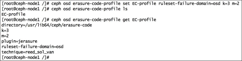
1. The command mentioned in this section will create an erasure code profile with the name EC-profile, which will have characteristics of k=3 and m=2, which are the number of data and coding chunks, respectively. So, every object that is stored in the erasure-coded pool will be divided into 3 (k) data chunks, and 2 (m) additional coding chunks are added to them, making a total of 5 (k + m) chunks. Finally, these 5 (k + m) chunks are spread across different OSD failure zones.

· Create the erasure code profile:

· # ceph osd erasure-code-profile set EC-profile ruleset-failure-domain=osd k=3 m=2

· List the profile:

· # ceph osd erasure-code-profile ls

· Get the contents of your erasure code profile:

· # ceph osd erasure-code-profile get EC-profile

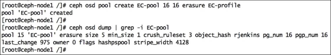
2. Create a Ceph pool of erasure type, which will be based on the erasure code profile that we created in step 1:

3. # ceph osd pool create EC-pool 16 16 erasure EC-profile

Check the status of your newly created pool; you should find that the size of the pool is 5 (k + m), that is, erasure size 5. Hence, data will be written to five different OSDs:

# ceph osd dump | grep -i EC-pool

Note

Use a relatively good number or PG_NUM and PGP_NUM for your Ceph pool, which is more appropriate for your setup.

4. Now we have a new Ceph pool, which is of type erasure. We should now put some data to this pool by creating a sample file with some random content and putting this file to a newly created erasure-coded Ceph pool:

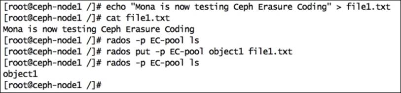
5. Check the OSD map for EC-pool and object1. The output of this command will make things clear by showing the OSD ID where the object chunks are stored. As explained in step 1, object1 is divided into 3 (m) data chunks and added with 2 (k) coded chunks; so, altogether, five chunks were stored on different OSDs across the Ceph cluster. In this demonstration, object1 has been stored on five OSDs, namely, osd.7, osd.6, osd.4, osd.8, and osd.5.

At this stage, we have completed setting up an erasure pool in a Ceph cluster. Now, we will deliberately try to break OSDs to see how the erasure pool behaves when OSDs are unavailable.

6. As mentioned in the previous step, some of the OSDs for the erasure pool are osd.4 and osd.5; we will now test the erasure pool reliability by breaking these OSDs one by one.

Note

These are some optional steps and should not be performed on Ceph clusters serving critical data. Also, the OSD numbers might change for your cluster; replace wherever necessary.

Bring down osd.4 and check the OSD map for EC-pool and object1. You should notice that osd.4 is replaced by a random number 2147483647, which means that osd.4 is no longer available for this pool:

# ssh ceph-node2 service ceph stop osd.5

# ceph osd map EC-pool object1

7. Similarly, break one more osd, that is, osd.5, and notice the OSD map for EC-pool and object1. You should notice that osd.5 is replaced by the random number 2147483647, which means that osd.5 is also no longer available for this pool:

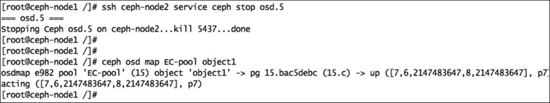
8. Now, the Ceph pool is running on three OSDs, which is the minimum requirement for this setup of erasure pool. As discussed earlier, the EC-pool will require any three chunks out of five in order to serve data. Now, we have only three chunks left, which are on osd.7, osd.6, and osd.8, and we can still access the data.

In this way, erasure coding provides reliability to Ceph pools, and at the same time, less amount of storage is required to provide the required reliability.

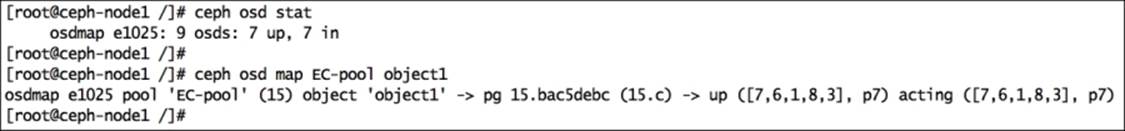
The Erasure code feature is greatly benefited by Ceph's robust architecture. When Ceph detects unavailability of any failure zone, it starts its basic operation of recovery. During the recovery operation, erasure pools rebuild themselves by decoding failed chunks on to new OSDs, and after that, they make all the chunks available automatically.

In the last two steps mentioned above, we intentionally broke osd.4 and osd.5. After a while, Ceph started recovery and regenerated missing chunks onto different OSDs. Once the recovery operation is complete, you should check the OSD map for EC-pool and object1; you will be amazed to see the new OSD ID as osd.1 and osd.3, and thus, an erasure pool becomes healthy without administrative input.

This is how Ceph and erasure coding make a great combination. The erasure coding feature for a storage system such as Ceph, which is scalable to the petabyte level and beyond, will definitely give a cost-effective, reliable way of data storage.

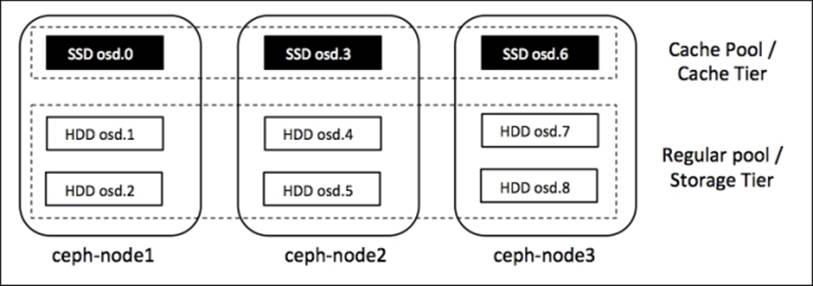
Ceph cache tiering

Like erasure coding, the cache tiering feature has also been introduced in the Ceph Firefly release, and it has been one of the most talked about features of Ceph Firefly. Cache tiering creates a Ceph pool that will be constructed on top of faster disks, typically SSDs. This cache pool should be placed in front of a regular, replicated, or erasure pool such that all the client I/O operations are handled by the cache pool first; later, the data is flushed to existing data pools.

The clients enjoy high performance out of the cache pool, while their data is written to regular pools transparently.

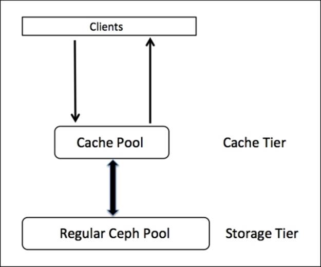
Generally, a cache tier is constructed on top of expensive/faster SSD disks, thus it provides clients with better I/O performance. The cache pool is backed up by a storage tier, which is made up of HDDs with type replicated or erasure. In this type of setup, clients submit I/O requests to the cache pool and get instant responses for their requests, whether it's a read or write; the faster cache tier serves the client request. After a while, the cache tier flushes all its data to the backing storage tier so that it can cache new requests from clients. All the data migration between the cache and storage tiers happens automatically and is transparent to clients. Cache tiering can be configured in two modes.

The writeback mode

When Ceph cache tiering is configured as a writeback mode, a Ceph client writes the data to the cache tier pool, that is, to the faster pool, and hence receives acknowledgement instantly. Based on the flushing/evicting policy that you have set for your cache tier, data is migrated from the cache tier to the storage tier, and eventually removed from the cache tier by a cache-tiering agent. During a read operation by the client, data is first migrated from the storage tier to the cache tier by the cache-tiering agent, and it is then served to clients. The data remains in the cache tier until it becomes inactive or cold.

The read-only mode

When Ceph cache tiering is configured as a read-only mode, it works only for a client's read operations. The client's write operation does not involve cache tiering, rather, all the client writes are done on the storage tier. During read operations by clients, a cache-tiering agent copies the requested data from the storage tier to the cache tier. Based on the policy that you have configured for the cache tier, stale objects are removed from them. This approach is idle when multiple clients need to read large amounts of similar data.

Implementing cache tiering

A cache tier is implemented on faster physical disks, generally SSDs, which makes a fast cache layer on top of slower regular pools made up of HDD. In this section, we will create two separate pools, a cache pool and a regular pool, which will be used as cache tier and storage tier, respectively:

Creating a pool

In Chapter 7, Ceph Operations and Maintenance, we discussed the process of creating Ceph pools on top of specific OSDs by modifying a CRUSH map. Similarly, we will create a cache pool, which will be based on osd.0, osd.3, and osd.6. Since we do not have real SSDs in this setup, we will assume the OSDs as SSDs and create a cache pool on top of it. The following are the instructions to create a cache pool on osd.0, osd.3, and osd.4:

1. Get the current CRUSH map and decompile it:

2. # ceph osd getcrushmap -o crushmapdump

3. # crushtool -d crushmapdump -o crushmapdump-decompiled

4. Edit the decompiled CRUSH map file and add the following section after the root default section:

5. # vim crushmapdump-decompiled

6. root cache {

7. id -5

8. alg straw

9. hash 0

10. item osd.0 weight 0.010

11. item osd.3 weight 0.010

12. item osd.6 weight 0.010

13.}

Tip

You should change the CRUSH map layout based on your environment.

14. Create the CRUSH rule by adding the following section under the rules section, generally at the end of the file. Finally, save and exit the CRUSH map file:

15.rule cache-pool {

16. ruleset 4

17. type replicated

18. min_size 1

19. max_size 10

20. step take cache

21. step chooseleaf firstn 0 type osd

22. step emit

23.}

24. Compile and inject the new CRUSH map to the Ceph cluster:

25.# crushtool -c crushmapdump-decompiled -o crushmapdump-compiled

26.# ceph osd setcrushmap -i crushmapdump-compiled

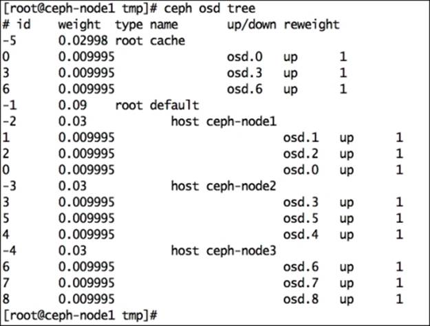
27. Once the new CRUSH map has been applied to the Ceph cluster, you should check the OSD status to view new OSD arrangements. You will find a new bucket root cache:

28.# ceph osd tree

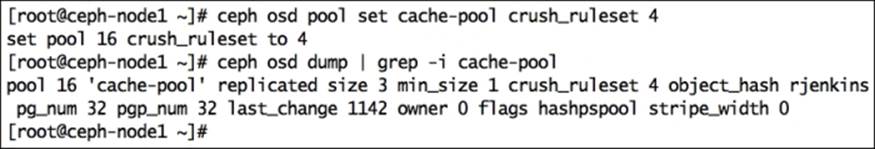
29. Create a new pool and set crush_ruleset as 4 so that the new pool gets created on SSD disks:

30.# ceph osd pool create cache-pool 32 32

31.# ceph osd pool set cache-pool crush_ruleset 4

Tip

We do not have real SSDs; we are assuming osd.0, osd.3, and osd.6 as SSDs for this demonstration.

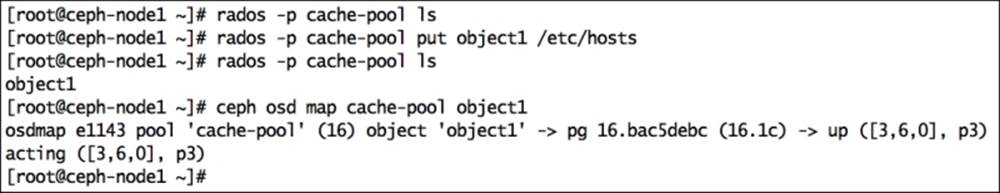
32. Make sure your pool is created correctly, that is, it should always store all the objects on osd.0, osd.3, and osd.6:

· List the cache-pool for contents; since it's a new pool, it should not have any content:

· # rados -p cache-pool ls

· Add a temporary object to the cache-pool to make sure that it's storing the object on the correct OSD:

· # rados -p cache-pool put object1 /etc/hosts

· List the contents of the cache-pool:

· # rados -p cache-pool ls

· Check the OSD map for cache-pool and object1. If you configured the CRUSH map correctly, object1 should get stored on osd.0, osd.3, and osd.6 as its replica size is 3:

· # ceph osd map cache-pool object1

· Remove the object:

· # rados -p cache-pool rm object1

Creating a cache tier

In the previous section, we created a pool based on SSDs; we will now use this pool as a cache tier for an erasure-coded pool named EC-pool that we created earlier in this chapter.

The following instructions will guide you through creating a cache tier with the writeback mode and setting the overlay with an EC-pool:

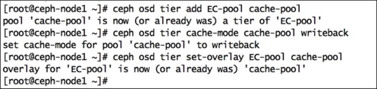
1. Set up a cache tier that will associate storage pools with cache-pools. The syntax for this command is ceph osd tier add <storage_pool> <cache_pool>:

2. # ceph osd tier add EC-pool cache-pool

3. Set the cache mode as either writeback or read-only. In this demonstration, we will use writeback, and the syntax for this is # ceph osd tier cache-mode <cache_pool> writeback:

4. # ceph osd tier cache-mode cache-pool writeback

5. To direct all the client requests from the standard pool to the cache pool, set the pool overlay, and the syntax for this is # ceph osd tier set-overlay <storage_pool> <cache_pool>:

6. # ceph osd tier set-overlay EC-pool cache-pool

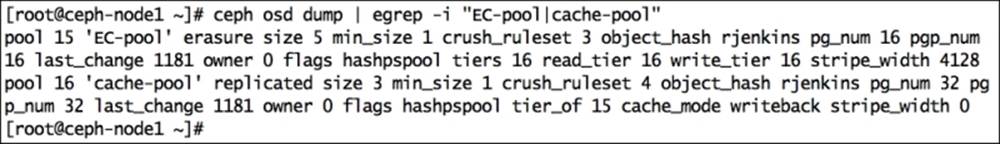
7. On checking the pool details, you will notice that the EC-pool has tier, read_tier, and write_tier set as 16, which is the pool ID for cache-pool.

Similarly, for cache-pool, the settings will be tier_of set as 15 and cache_mode as writeback; all these settings imply that the cache pool is configured correctly:

# ceph osd dump | egrep -i "EC-pool|cache-pool"

Configuring a cache tier

A cache tier has several configuration options; you should configure your cache tier in order to set policies for it. In this section, we will configure cache tier policies:

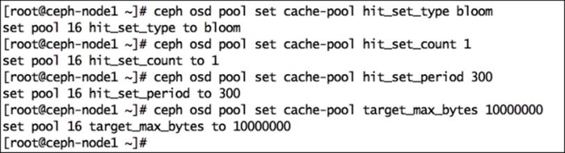
1. Enable hit set tracking for the cache pool; the production-grade cache tier uses bloom filters:

2. # ceph osd pool set cache-pool hit_set_type bloom

3. Enable hit_set_count, which is the number of hits set to store for a cache pool:

4. # ceph osd pool set cache-pool hit_set_count 1

5. Enable hit_set_period, which is the duration of the hit set period in seconds to store for a cache pool:

6. # ceph osd pool set cache-pool hit_set_period 300

7. Enable target_max_bytes, which is the maximum number of bytes after the cache-tiering agent starts flushing/evicting objects from a cache pool:

8. # ceph osd pool set cache-pool target_max_bytes 1000000

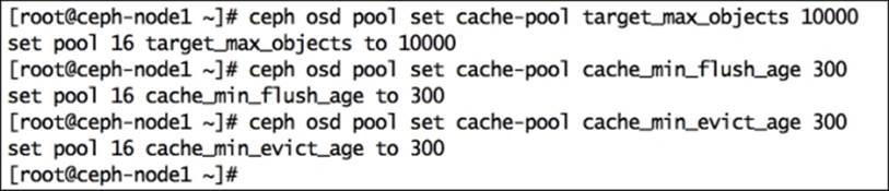
9. Enable target_max_objects, which is the maximum number of objects after which a cache-tiering agent starts flushing/evicting objects from a cache pool:

10.# ceph osd pool set cache-pool target_max_objects 10000

11. Enable cache_min_flush_age and cache_min_evict_age, which are the time in seconds a cache-tiering agent will take to flush and evict objects from a cache tier to a storage tier:

12.# ceph osd pool set cache-pool cache_min_flush_age 300

13.# ceph osd pool set cache-pool cache_min_evict_age 300

14. Enable cache_target_dirty_ratio, which is the percentage of cache pool containing dirty (modified) objects before the cache-tiering agent flushes them to the storage tier:

15.# ceph osd pool set cache-pool cache_target_dirty_ratio .01

16. Enable cache_target_full_ratio, which is the percentage of cache pool containing unmodified objects before the cache-tiering agent flushes them to the storage tier:

17.# ceph osd pool set cache-pool cache_target_full_ratio .02

18. Create a temporary file of 500 MB that we will use to write to the EC-pool, which will eventually be written to a cache-pool:

19.# dd if=/dev/zero of=/tmp/file1 bs=1M count=500

Tip

This is an optional step; you can use any other file to test cache pool functionality.

The following screenshot shows the preceding commands in action:

Testing the cache tier

Until now, we created and configured a cache tier. Next, we will test it. As explained earlier, during a client write operation, data seems to be written to regular pools, but actually, it is written on cache-pools first, therefore, clients benefit from the faster I/O. Based on the cache tier policies, data is migrated from a cache pool to a storage pool transparently. In this section, we will test our cache tiering setup by writing and observing the objects on cache and storage tiers:

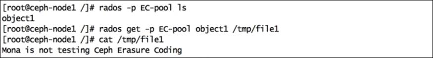
1. In the previous section, we created a 500 MB test file named /tmp/file1; we will now put this file to an EC-pool:

2. # rados -p EC-pool put object1 /tmp/file1

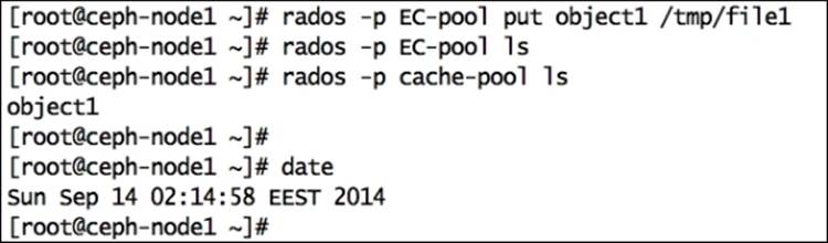
3. Since an EC-pool is tiered with a cache-pool, file1 should not get written to the EC-pool at the first state. It should get written to the cache-pool. List each pool to get object names. Use the date command to track time and changes:

4. # rados -p EC-pool ls

5. # rados -p cache-pool ls

6. # date

7. After 300 seconds (as we have configured cache_min_evict_age to 300 seconds), the cache-tiering agent will migrate object1 from the cache-pool to EC-pool; object1 will be removed from the cache-pool:

8. # rados -p EC-pool ls

9. # rados -p cache-pool ls

10.# date

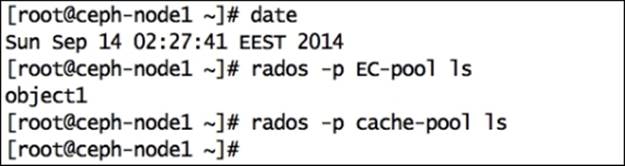
As explained in the preceding output, data is migrated from a cache-pool to an EC-pool after a certain time.

Ceph benchmarking using RADOS bench

Ceph comes with an inbuilt benchmarking program known as RADOS bench, which is used to measure the performance of a Ceph object store. In this section, we will make use of RADOS bench to get the performance metrics of our Ceph cluster. As we used virtual, low configuration nodes for Ceph, we should not expect good performance numbers with RADOS bench in this demonstration. However, one can get good performance results if they are using recommended hardware with performance-tuned Ceph deployment.

The syntax to use this tool is rados bench -p <pool_name> <seconds> <write|seq|rand>.

The valid options for rados bench are as follows:

· -p or --pool: This is the pool name

· <Seconds>: This is the number of seconds a test should run

· <write|seq|rand>: This is the type of test; it should either be write, sequential read, or random read

· -t: This is the number of concurrent operations; the default is 16

· --no-cleanup: The temporary data that is written to pool by RADOS bench should not be cleaned. This data will be used for read operations when used with sequential reads or random reads. The default is cleaned up.

Using the preceding syntax, we will now run some RADOS bench tests:

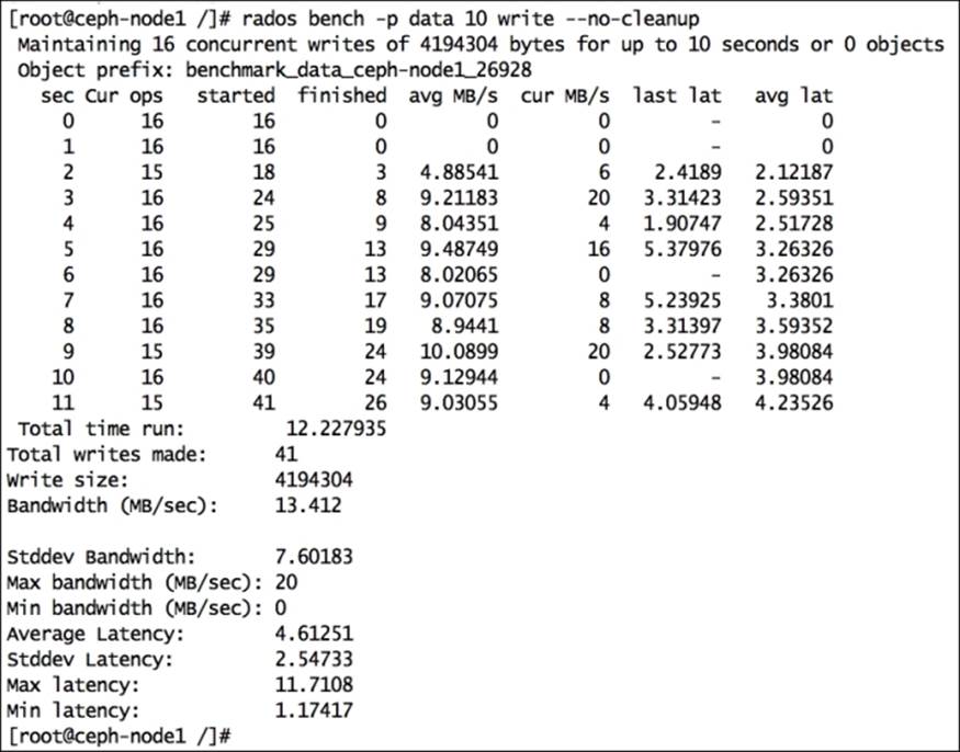
· A 10-second write test on a data pool will generate the following output. The important thing to note in RADOS bench output is bandwidth (MB/sec), which is 13.412 for our setup, which is very low as it's a virtual Ceph cluster. Other things to watch out for are total writes made, write size, average latency, and so on. As we are using the --no-cleanup flag, the data written by RADOS bench will not be erased, and it will be used by sequential and random read operations by RADOS bench:

· # rados bench -p data 10 write --no-cleanup

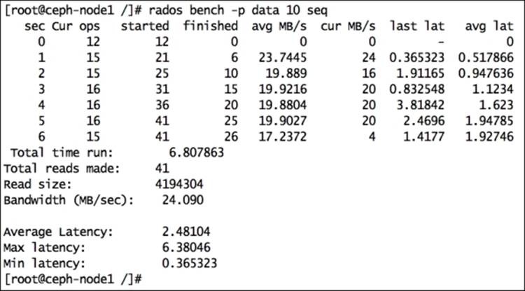
· Perform a sequential read benchmarking test on the data pool:

· # rados bench -p data 10 seq

· Perform a random read benchmarking test on the data pool:

· # rados bench -p data 10 rand

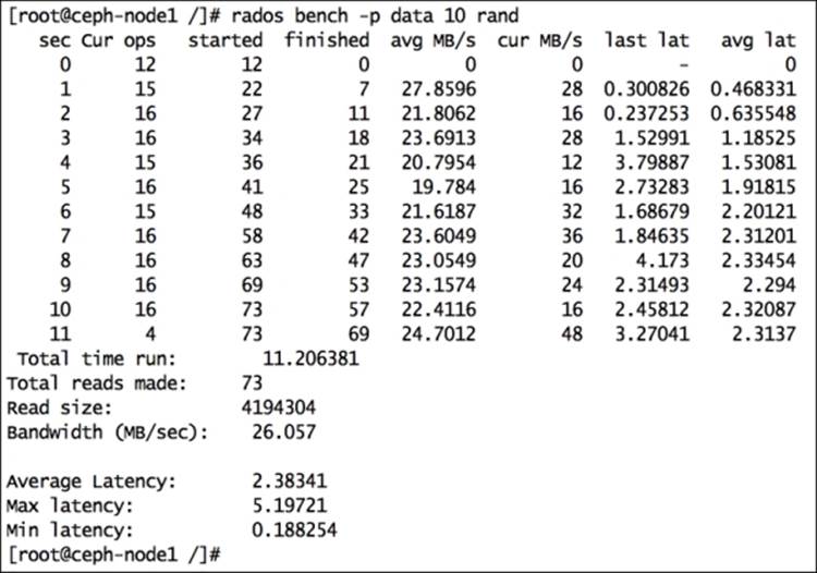
In this way, you can creatively design your test cases based on write, read, and random read operations for your Ceph pool. RADOS bench is a quick-and-easy benchmarking utility, and the good part is that it comes bundled with Ceph.

Summary

Performance tuning and benchmarking make your Ceph cluster production class. You should always fine-tune your Ceph cluster before moving it to production usage from preproduction, development, or testing. Performance tuning is a vast subject, and there is always a scope of tuning in every environment. You should use performance tools to meter the performance of your Ceph cluster, and based on the results, you can take necessary actions.

In this chapter, have reviewed most of the tuning parameters for your cluster. You have learned advanced topics such as performance tuning from hardware as well as software perspectives. This chapter also included a detailed explanation on Ceph erasure coding and cache-tiering features, followed by the Ceph inbuilt benchmarking tool, RADOS bench.