Better Business Decisions from Data: Statistical Analysis for Professional Success (2014)
Part II. Data
Chapter 5. The Raw Data
Hard to Digest Until Processed
Raw data is the expression used to describe the original data before any analysis is undertaken. It is not a very palatable phrase. Something like “original data” or “new data” would have been more inviting, but I have to stick to convention. The purpose of this chapter is to explain the different kinds of data and present a number of definitions to be used in the chapters that follow. In addition, I will demonstrate how figures can mislead or confuse even before the statistical analysis has started.
Descriptive or Numerical
Data may be descriptive or numerical. Descriptive data, which is also called categorical, can be placed in categories and counted. Recording the way people vote in an election, for example, requires the categories—namely, the political parties—to be defined, and each datum adds one more to the appropriate category. The process of counting produces numerical values which summarize the data and can be used in subsequent processing. Thus we can express voting results as proportions of voters for each of the political parties.
If descriptive data can be placed in order but without any way of comparing the sizes of the gaps between the categories, the data is said to be ordinal. Thus we can place small, medium, and large in order, but the difference between small and medium may not be the same as the difference between medium and large. The placing in order in this way is referred to as ranking. Not only can the numbers in each category be totaled to give numerical values, but it also may be possible to attribute ordered numbers to each category. Thus small, medium, and large could be expressed respectively as 1, 2, and 3 on a scale indicating increasing size, to allow further processing.
Descriptive data that cannot be placed in order is called nominal. Examples include color of eyes and place of birth. Collections of such data consist of numbers of occurrences of the particular attribute. If just two categories are being considered and they are mutually exclusive (for example, yes/no data), the data is referred to as binomial.
Numerical data may be continuous or discrete. Continuous data can be quoted to any degree of accuracy on an unbroken scale. Thus 24.31 km, 427.4 km, and 5017 km are examples of distances expressed as continuous numerical data. Discrete data can have only particular values on a scale that has gaps. Thus the number of children in a family can have values of 0, 1, 2, 3, 4, …, with no in-between values. Notice that there is still a meaningful order of the values, as with continuous data.
Strictly speaking, continuous data becomes discrete once it is rounded, because it is quoted to a finite number of digits. Thus 24.31 is a discrete value located between 24.30 and 24.32. However, this is a somewhat pedantic observation and unlikely to cause problems. Of more importance is recognition of the fact that discrete data can often be processed as if the data were continuous, as you will see in Chapter 11.
Within a set of data there are usually several recorded features: numerical, descriptive, or both. Each feature—for example, cost or color—is referred to as a variable. The term random variable is often used to stress the fact that the values that the variables have are a random selection from the potentially available values.
A distribution is the set of values of the variable represented in a sample or a population, together with the frequency or relative frequency with which each value occurs. Thus, a listing of shoe sizes for a group of 50 men might show the following:
Shoe size: 8, 9, 8, 7, 9, 9, 8, 6, 10, 9, 10, 7, 9, 6, 11, 9, 8, 8, 7,9, 9, 6,10, 9, 8, 9, 10, 8,
7, 9, 6, 7, 8, 10, 7,10, 9, 9, 10, 8, 7, 8, 9, 7, 10, 9, 8, 7, 8, 9
The values, 50 in total, can be counted and grouped as follows:
|
Shoe Size |
Number of Men (Frequency) |
|
6 |
4 |
|
7 |
9 |
|
8 |
12 |
|
9 |
16 |
|
10 |
8 |
|
11 |
1 |
The distribution can be shown diagrammatically in the form of a bar chart, as in Figure 5-1. The values can be seen to cluster around the central values. Starting in Chapter 7, I will discuss such distributions in more detail. In particular, you will meet the so-called normal distribution, which is of this form and which plays a major part in statistical analysis.
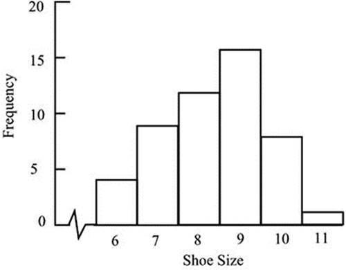
Figure 5-1. Bar chart showing the distribution of shoe sizes in a sample of 50 men
Some distributions are quite irregular in appearance when shown as bar charts. Others, including the normal distribution, not only are regular but also can be described exactly by mathematical formulae. Some of these will be encountered in Chapters 7, 11, and 18.
Format of Numbers
We are all familiar with the numbers we meet in our daily lives. Generally, these are neither too small nor too large for us to easily visualize them. However, very large or very small numbers can be a source of confusion.
Because large numbers written in full are very long, scientific reports adopt a shorthand method called standard index form. Multiplication factors of 10 are indicated by a superscript. So a million is 106, meaning 10 × 10 × 10 × 10 × 10 × 10. The number 2,365,000 can be written as 2.365x10⁶. It is useful to note that the superscript, 6 in this case, indicates the number of moves of the decimal point to the right that are required to restore the number to the usual format.
Owing in part to computer literacy, the prefixes that are used in scientific work are creeping into common usage even in metrically challenged countries such as the United States. These prefixes are the set of decadic (decimal-based) multiples applied to the so-called SI units (abbreviated fromLe Systéme internationale d’unités). Thus kilo, or simply k, is taken to mean 1000—so we see $3k, meaning $3000. Mega means a million and has the abbreviation M in scientific work; but in financial documents we see the abbreviation MM, such that $8MM is taken to mean $8,000,000. To add to the confusion, MM is the Roman numeral for 2000. Further up the scale we have giga (G) for 1000 millions (109), but in financial writing we see $1B, $1BN, or $1bn. Giga became increasingly popularized after consumer hard disk storage capacity crossed into the gigabyte (GB) range in the 1990s. The next prefixes up, tera (T) for a million millions (1012) and peta (P), which is a thousand times larger again (1015), are used in relation to big data, which I will discuss in Part VII.
The superscripts in 106 and so on are referred to as orders of magnitude. Each added factor of ten indicates the next order of magnitude. To say that two numbers are of the same order of magnitude means they are within a factor of ten of each other.
Very small numbers are encountered less frequently than very large ones. We seem to have no special traditional names for the small numbers except the awkward fraction words like hundredth, thousandth, etc. The standard index form described above extends to the very small, the superscripts being negative and indicating division by a number of tens rather than multiplication. Thus, 10–3 means 1 divided by 1000—that is, 10–3 means “one thousandth.” The number 0.00000378 may be written as 3.78x10⁻⁶, meaning 3.78 divided by 10 six times. As with the large numbers, the superscript, –6 in this case, indicates the number of moves of the decimal point that are required to restore the number to the usual format—except that the moves are now to the left, as indicated by the negative sign.
As with the large numbers, prefixes indicate how many tens the number shown has to be divided by. Some of these are in common use. One hundredth (0.01 or 10–2) is indicated by centi (c). One thousandth (0.001 or 10–3) is indicated by milli (m), and one millionth (0.000001 or 10–6) bymicro (the Greek letter µ, pronounced “mu”). The prefix nano (n) is encountered in the fashionable word nanotechnology, which is the relatively new branch of science dealing with molecular sizes. Nano indicates one thousand-millionth (0.000000001 or 10–9), one nanometer (1 nm) being about the size of a molecule. Other SI prefixes used in the scientific community but not yet broadly encountered are pico (p) for one million-millionth (10–12), femto (f) for one thousand-million-millionth (10–15), and atto (a) for one million-million-millionth (10–18).
Figure 5-2 brings together the various prefixes mentioned, together with a few even more exotic ones.
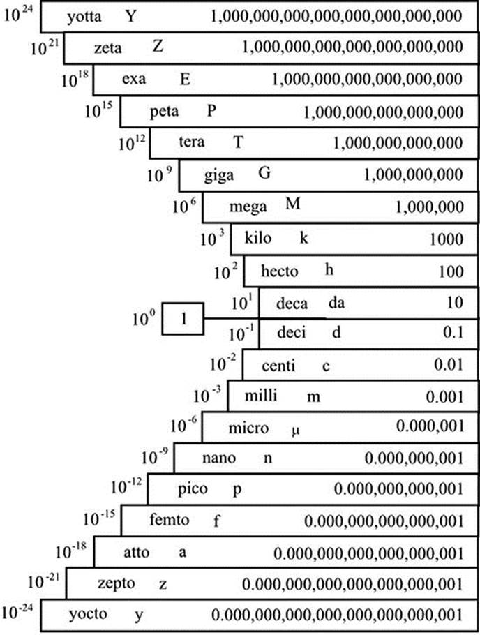
Figure 5-2. Prefixes used to denote decadic multiples or fractions of units
Negative numbers are well understood, but beware of possible confusion when comparing two negative numbers. If sales decrease by 200 units in January and by 300 in February, the change is said to be greater in February than in January. However, –300 is mathematically less than –200.
Multiplying or dividing two negative numbers gives a positive number. For example, if I buy and sell some shares at the same price, and the share price then changes, my profit is the excess number bought multiplied by the increase. Written as a formula, it is
Profit=(B–S)´P
where B is the number bought, S is the number sold, and P is the increase in price. Four situations might be as follows:
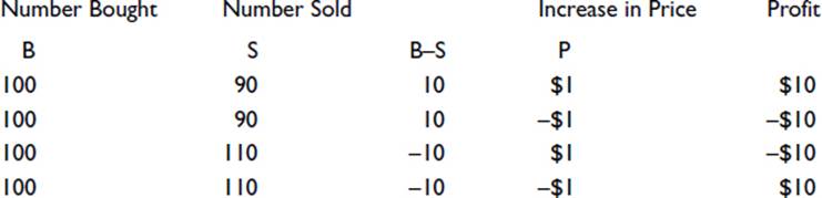
The profit is negative if either the number sold is greater than the number bought or the price decreases. However, if both of these occur, as shown in the bottom line, the profit is positive.
In financial reports, negative values are avoided whenever possible. I have often wondered why this is so. It seems so odd in bookkeeping that, when balancing books, two columns (debit and credit) have to be added separately and then compared and the smaller subtracted from the larger. The result, always positive, is then added to the column with the smaller total to effect a balance, thus completely avoiding any recording of a negative value. Bookkeeping has a long history, and today’s rules and procedures date back to medieval times. Perhaps the negative sign in mathematics was then less commonly used. Alternatively, it may be because when adding a list of figures that includes negatives, the negative sign, being at the left side, may not be noticed until it is too late. When a final value, which happens to be negative, has to be quoted, it is placed in brackets. This too is odd, as brackets have a particular and different meaning in mathematics. At one time, such negative values were generally shown in red, and sometimes still are—hence the expression “in the red,” meaning overdrawn at the bank.
Rounding
Rounding is usually to the nearest value of the retained last digit. Thus, 4372 would be rounded to 4370 to the nearest ten 4400 to the nearest hundred or 4000 to the nearest thousand. When the digit to be removed is 5, it is common practice to round up, so 65 would become 70 to the nearest ten. It should be noted, however, that this can lead to a bias. In a list of numbers, each having a random final digit to be removed by rounding, more will be rounded up than down. If the numbers are subsequently added together, the total will be greater than the total of the original values. Inconsistencies can arise. If we calculate 10% of $5.25, we get $0.53 rounded up to the nearest penny. But 90%, calculated in the same way, gives $4.73, making the total slightly greater than the original amount. There are alternative methods of dealing with numbers ending with the digit 5 if the particular circumstances make it necessary. For example, in a long list of numbers, those ending in 5 can be rounded up and down alternately.
Raw statistical data that express continuously variable attributes will have been rounded, perhaps because the method of obtaining the values is limited in precision. Weighing precision, for example, is limited by the accuracy of the scales used. Or rounding may have been employed because the minor variations in the values are not considered to have any significance, either in the statistical processing that follows or in the conclusions that are expected following the processing.
Although rounding to the nearest retained last digit is usual, there are situations where always rounding up or always rounding down is adopted. The tax authorities in the UK and Singapore, for example, give the benefit to taxpayers of rounding down income and allowances and rounding up deductions.
Note that some values that appear to be discrete have in fact been rounded. A person’s age could be expressed to the nearest day, hour, minute or even closer, but in a statistical list it may be given as an integral year. Furthermore, the rounding is not usually to the nearest year, but to the age last birthday. This makes no difference in many instances, of course, but if we were, for example, considering children between the ages of 8 and 14, we could find that our sample included children from just 8 years old to 15 years old less one day.
Rounding always creates discrete values, of course, but the small intervals relative to the size of the values render the values continuous in effect.
As a general principle, rounding should be carried out at the end of a calculation and not part way through, if errors are to be avoided. Successive roundings can give rise to cumulative errors. If we start, for example, with the number 67 and subject it to a number of arithmetic operations, we must wait until the final operation before rounding the answer to the required digit. Suppose we divide it by 5 and then multiply the answer by 7. We get 93.8, which we round to the nearest whole number, 94. If, alternatively, we round to the nearest whole number after the first operation, the sequence runs as follows: 67 divided by 5 is 13.4, which we round to 13; multiplying by 7 gives 91, which is incorrect.
Difficulties can arise if figures that have already been rounded are taken from sources and processed further. If, to take an extreme example, we read that 20 million cars are registered as being in use on the roads, but we see elsewhere that records show only 18 million currently licensed, we might view the difference and deduce that 2 million, or 10%, are unlicensed. In reality, the figure could be almost as low as half this if the original data—19.51 million registered and 18.49 million licensed—had been rounded to the nearest million. When figures that appear to be rounded are required for further analysis, the maximum and minimum possible values that they may represent should be examined. Unless the worst case combination of the values is inconsequential, it is wise to seek the original data.
I wonder about rounding whenever I hear a time check on the radio. When the announcer says, “It is now sixteen minutes past two”—does he mean “exactly 16 minutes past 2:00”? Or does he mean “correct to the nearest minute”—in which case it could be anything between 15.5 minutes past to 16.5 past? Or he may mean that his digital clock is showing 16 minutes past and the actual time is somewhere between 16 and 17 minutes past. Not that it usually matters, of course.
Percentages
Any number can be represented by a fraction, a decimal, or a percentage. Thus ½ = 0.5 = 50%. To obtain a decimal from a fraction, divide the top by the bottom. To turn either into a percentage, multiply by 100. Expressing numbers as percentages in this way is useful when the numbers are less than 1. For numbers greater than 1, there is no advantage but it is done for effect. The number 2 is 200%. Notice the difference between sales increasing by 200% compared with last year and sales increasing to 200% compared with last year. In the first situation, sales have trebled; in the second, they have doubled.
Increases or decreases in sales, income, tax, and so on can be quoted as percentages or as actual values. The impression given can change enormously depending on which is chosen. A small increase of a small value can be a large percentage. A family with one child has a 100% increase in the number of children when the second child is born. A family with 5 children has only a 20% increase when the next one is born. Similarly, a large increase of a large value can be a small percentage. An annual salary increase of $1,000 for somebody earning half a million dollars is only 0.2%, whereas for a full-time worker making the federal minimum wage, it is 7%.
If you read that manufacturing has reduced from 25% of economic output to 12% in the last 20 years, you may well conclude that the amount of manufacturing has reduced. This is not necessarily so. It could actually have increased in absolute terms, its percentage reduction being due to a large increase in another sector of the economy. When data are presented as percentage changes, it is worth examining how the data would look in the form of actual changes.
Ages are usually quoted to the nearest year, but children appreciate that one year is a large proportion of their ages. You hear, “I am nine and a half, but next week I shall be nine and three quarters.” Quoting the age of a ten-year-old to the nearest quarter of a year seems pedantic, yet it is less precise, as a percentage, than reporting the ages of pensioners to the nearest year.
Richard Wiseman (2007: 128) gives an interesting example of how people perceive values differently when seen as percentages. In the first scenario, a shopper is buying a calculator costing $20. Immediately before the purchase takes place, the shop assistant says that tomorrow there is a sale and the calculator will cost only $5. The shopper has to decide whether to proceed with the purchase or return to the shop tomorrow. In the second scenario, the shopper is buying a computer costing $999. This time, the assistant explains that tomorrow the cost will be only $984. On putting these scenarios to people, researchers have found that about 70% say they would put off buying the calculator until tomorrow but would go ahead with the purchase of the computer immediately. Yet the saving from delaying is the same in each situation—namely, $15.
This choice between percentage changes and actual changes impinges not only on the presentation of data, but on many issues that affect daily life. Should a tax reduction be a percentage or a fixed value for all? Should a pay rise be a percentage across the board or the same amount for everyone? These questions create lots of debate but little agreement. In reality, a compromise somewhere between the two usually results.
Note that a percentage is always calculated on the basis of the original value. So if my income increases by 10% this year but decreases by 10% next year, I end up with a lower income, because the second calculation is based on a higher income, and the 10% reduction represents more than the earlier increase of 10% did. In a similar way if I purchase stock that has been reduced by 20% and pay $1000, my saving is not $200 but rather more, because the reduction was calculated as a percentage of the original price.
A company having reduced the usage of paper, with the evidence that 12 boxes which were previously used in 4 days now last 6 days, may claim a 50% reduction. At a glance, it may look like 50%, because 6 days is 50% more than 4 days. However, the original usage was 3 boxes per day, and it is now 2 boxes per day—i.e., a reduction of 1 in 3, or 33%.
Sometimes there is ambiguity regarding which is the original value, and this can allow some bias in quoting the result. Suppose my car does 25 miles per gallon of fuel and yours does 30 miles per gallon. You would be correct in saying that your fuel consumption is 20% ((30 – 25) × 100/25) better than mine, the wording implying that it is your consumption that is being calculated, using my consumption as the base value. However, I would be equally correct in saying that my fuel consumption is only 16.7% ((30 – 25) × 100/30) worse than yours, calculating my consumption with yours as the base value.
Also deceptive is the way percentage rates of increase or decrease change as the time period considered increases. If the monthly interest rate on my credit card balance is 2%, I need to know what this is equivalent to when expressed as an annual rate. A debt of P will have risen to P × (1 + 2/100) at the end of the first month. At the end of the second month, this sum has to be multiplied by (1 + 2/100) to get the new total. By the end of the year, the original balance will have been multiplied by this factor 12 times. The final figure is 1.268 × P: an increase of nearly 27% compared with the quick-glance impression of 24%. Many will recognize this as a compound interest calculation and will be familiar with a formula that allows a quicker way of arriving at the result. Those not familiar with the calculation will nevertheless recognize with some pleasure that their bank accounts show this feature in producing increasing interest each year, even without additional deposits being made.
Confusion can arise when a percentage of a percentage is calculated. If the standard rate of tax is 20%, say, and the chancellor decides to increase it by 5%, the new rate will not be 25% but 21%. If he wished to be really unpopular and increase the rate to 25%, he could say that the rate would be increased by 5 percentage points, rather than by 5 percent.
Simple Index Numbers
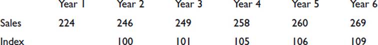
Index numbers are used to render a trend in a sequence of values more easily appreciated. Thus we might have, say, the number of washing machines sold by a shop each year, as follows:
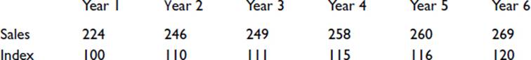
Year 1 has been adopted as the base, so the index is shown as 100. The succeeding indices are obtained by expressing each sales value as a percentage of the base value. Thus, for Year 2, (246/224) × 100 = 110.
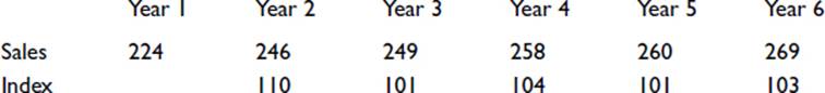
The impression given to the reader depends very greatly on what has been chosen as the base value. If we look again at the above values but now take Year 2 as the base value, we get the following sequence:
The increasing sales now look less impressive.
A fair picture will emerge, provided the chosen base is typical in the appropriate sense. We would really need to know whether the sales for Year 1 were unusually low or whether they represented an increase on previous years.
A chain index can be calculated using each previous value as the base instead of the initial value. Thus for the above sales figures, we would have the following:
In such sequences, favorable indices tend to be followed by unfavorable ones, and vice versa. The sequence has the advantage of better illustrating a rate of change. A steady rise in sales or a steady fall in sales would be shown by a sequence of similar values. A sequence of rising values would indicate an increasing rate of increase in sales, whereas a sequence of falling values would indicate an increasing rate of decreasing sales.
All materials on the site are licensed Creative Commons Attribution-Sharealike 3.0 Unported CC BY-SA 3.0 & GNU Free Documentation License (GFDL)
If you are the copyright holder of any material contained on our site and intend to remove it, please contact our site administrator for approval.
© 2016-2026 All site design rights belong to S.Y.A.