Data Science For Dummies (2016)

Part 4

Computing for Data Science

IN THIS PART …

Find out how Python is being used for data science projects.

Look at your open-source data science options. (Can you say “R”?)

See how SQL can be put to new (data science) uses.

Explore old programs (Excel) and new (KNIME).

Chapter 14

Using Python for Data Science

IN THIS CHAPTER

Taking on data types

Looking at how loops work

Forming simple user-defined functions

Defining classes in Python

Exploring data science Python libraries

Practicing data analysis for yourself

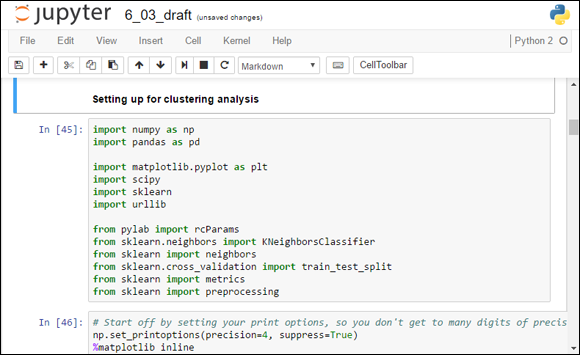
Although popular programming languages like Java and C++ are good for developing stand-alone desktop applications, Python’s versatility makes it an ideal programming language for processing, analyzing, and visualizing data. For this reason, Python has earned a reputation of excellence in the data science field, where it has been widely adopted over the past decade. In fact, Python has become so popular that it seems to have stolen ground from R — the other free, widely adopted programming language for data science applications. Python’s status as one of the more popular programming languages out there can be linked to the fact that it’s relatively easy to master and it allows users to accomplish several tasks using just a few lines of code.

In this chapter, I first introduce you to the fundamental concepts of programming with Python (such as data types, function, and classes), and then I present the information you need to know to set up a standard Python working environment in Jupyter. I also introduce some of the best Python libraries for manipulating data, performing statistical computations, creating data visualizations, and completing other related tasks. Lastly, I walk you through some scenarios designed to illustrate how Python can best help you analyze data.

You can use Python to do anything, from simple mathematical operations to data visualization and even machine learning and predictive analytics. Here’s an example of a basic math operation in Python (Figure 14-1 shows an example — taken from Python’s MatPlotLib library — of a more advanced output):

>>> 2.5+3
5.5

FIGURE 14-1: Sample output from Python’s MatPlotLib library.

Regardless of the task at hand, you should always study the most basics concepts of a language before attempting to delve into its more specialized libraries.

Because Python is an object-oriented programming language, everything in Python is considered an object. In Python, an object is anything that can be assigned to a variable or passed as an argument to a function. The following items are all considered objects in the Python programming language:

· Numbers

· Strings

· Lists

· Tuples

· Sets

· Dictionaries

· Functions

· Classes

Additionally, all these items except for the last two in the list function as basic data types in plain ol’ Python, which is Python with no external extensions added to it. (I introduce you to the external Python libraries NumPy, SciPy, Pandas, MatPlotLib, and Scikit-learn in the section “Checking Out Some Useful Python Libraries,” later in this chapter; when you add these libraries, additional data types become available to you.)

In Python, functions do basically the same thing as they do in plain math — they accept data inputs, process them, and output the result. Output results depend wholly on the task the function was programmed to do. Classes, on the other hand, are prototypes of objects that are designed to output additional objects.

If your goal is to write fast, reusable, easy-to-modify code in Python, you must use functions and classes. Doing so helps to keep your code efficient and organized.

Sorting Out the Python Data Types

If you do much work with Python, you need to know how to work with different data types. The main data types in Python and the general forms they take are described in this list:

· Numbers: Plain old numbers, obviously

· Strings: ‘…’ or “…”

· Lists: […] or […, …, … ]

· Tuples: (…)

· Sets: Rarely used

· Dictionaries: {‘Key’: ‘Value’, …}.

Numbers and strings are the most basic data types. You can incorporate them inside other, more complicated data types. All Python data types can be assigned to variables.

In Python, numbers, strings, lists, tuples, sets, and dictionaries are classified as both object types and data types.

Numbers in Python

The numbers data type represents numeric values that you can use to handle all types of mathematical operations. Numbers come in the following types:

· Integers: A whole-number format

· Long: A whole-number format with an unlimited digit size

· Float: A real-number format, written with a decimal point

· Complex: An imaginary-number format, represented by the square root of -1

Strings in Python

Strings are the most often used data type in Python — and in every other programming language, for that matter. Simply put, a string consists of one or more characters written inside single or double quotes. The following code represents a string:

>>> variable1=’This is a sample string’
>>> print(variable1)
This is a sample string

In this code snippet, the string is assigned to a variable, and the variable subsequently acts like a storage container for the string value.

To print the characters contained inside the variable, simply use the predefined function, print.

Python coders often refer to lists, tuples, sets, and dictionaries as data structures rather than data types. Data structures are basic functional units that organize data so that it can be used efficiently by the program or application you’re working with.

Lists, tuples, sets, and dictionaries are data structures, but keep in mind that they’re still composed of one or more basic data types (numbers and/or strings, for example).

Lists in Python

A list is a sequence of numbers and/or strings. To create a list, you simply enclose the elements of the list (separated by commas) within square brackets. Here’s an example of a basic list:

>>> variable2=["ID","Name","Depth","Latitude","Longitude"]
>>> depth=[0,120,140,0,150,80,0,10]
>>> variable2[3]
'Latitude'

Every element of the list is automatically assigned an index number, starting from 0. You can access each element using this index, and the corresponding value of the list will be returned. If you need to store and analyze long arrays of data, use lists — storing your data inside a list makes it fairly easy to extract statistical information. The following code snippet is an example of a simple computation to pull the mean value from the elements of the depth list created in the preceding code example:

>>> sum(depth)/len(depth)
62.5

In this example, the average of the list elements is computed by first summing up the elements, via the sum function, and then dividing them by the number of the elements contained in the list. See, it’s as simple as 1-2-3!

Tuples in Python

Tuples are just like lists, except that you can’t modify their content after you create them. Also, to create tuples, you need to use normal brackets instead of squared ones. Here’s an example of a tuple:

>>> depth=(0,120,140,0,150,80,0,10)

In this case, you can’t modify any of the elements, like you would with a list. If you want to ensure that your data stays in a read-only format, use tuples.

Sets in Python

A set is another data structure that’s similar to a list. In contrast to lists, however, elements of a set are unordered. This disordered characteristic of a set makes it impossible to index, so it’s not a commonly used data type.

Dictionaries in Python

Dictionaries are data structures that consist of pairs of keys and values. In a dictionary, every value corresponds to a certain key, and consequently, each value can be accessed using that key. The following code snippet shows a typical key/value pairing:

>>> variable4={"ID":1,"Name":"Valley City","Depth":0,"Latitude":49.6, "Longitude":-98.01}
>>> variable4["Longitude"]
-98.01

Putting Loops to Good Use in Python

When working with lists in Python, you typically access a list element by using the element index number. In a similar manner, you can access other elements of the list by using their corresponding index numbers. The following code snippet illustrates this concept:

>>>variable2=["ID","Name","Depth","Latitude","Longitude"]
>>> print(variable2[3])
Latitude
>>> print(variable2[4])
Longitude

Don’t let the index numbering system confuse you. Every element of the list is automatically assigned an index number starting from 0 — not starting from 1. That means the fourth element in an index actually bears the index number 3.

When you’re analyzing considerable amounts of data and you need to access each element of a list, this technique becomes quite inefficient. In these cases, you should use a looping technique instead.

You can use looping to execute the same block of code multiple times for a sequence of items. Consequently, rather than manually access all elements one by one, you simply create a loop to automatically iterate (or pass through in successive cycles) each element of the list.

You can use two types of loops in Python: the for loop and the while loop. The most often used looping technique is the for loop — designed especially to iterate through sequences, strings, tuples, sets, and dictionaries. The following code snippet illustrates a for loop iterating through the variable2 list created in the preceding code:

>>> for element in variable2:print(element)
ID
Name
Depth
Latitude
Longitude

The other available looping technique in Python is the while loop. Use a while loop to perform actions while a given condition is true.

Looping is crucial when you work with long arrays of data, such as is the case when working with raster images. Looping allows you to apply certain actions to all data or to apply those actions to only predefined groups of data.

Having Fun with Functions

Functions (and classes, which I describe in the following section) are the crucial building blocks of almost every programming language. They provide a way to build organized, reusable code. Functions are blocks of code that take an input, process it, and return an output. Function inputs can be numbers, strings, lists, objects, or functions. Python has two types of functions: built-in and custom. Built-in functions are predefined inside Python. You can use them by just typing their names.

The following code snippet is an example of the built-in function print:

>>> print("Hello")
Hello

The highly used built-in function print prints out a given input. The code behind print has already been written by the people who created Python. Now that this code stands in the background, you don’t need to know how to code it yourself — you simply call the print function. The people who created the Python library couldn’t guess every possible function to satisfy everyone’s needs, but they managed to provide users with a way to create and reuse their own functions when necessary.

In the section “Sorting Out the Python Data Types,” earlier in this chapter, the code snippet from that section (listed again here) was used to calculate the average of elements in a list:

>>> depth=[0,120,140,0,150,80,0,10]
>>> sum(depth)/len(depth)
62.5

The preceding data actually represents snowfall and snow depth records from multiple point locations. As you can see, the points where snow depth measurements were collected have an average depth of 62.5 units. These are depth measurements taken at only one time, though. In other words, all the data bears the same timestamp. When modeling data using Python, you often see scenarios in which sets of measurements were taken at different times — known as time-series data.

Here’s an example of time-series data:

>>> december_depth=[0,120,140,0,150,80,0,10]
>>> january_depth=[20,180,140,0,170,170,30,30]
>>> february_depth=[0,100,100,40,100,160,40,40]

You could calculate December, January, and February average snow depth in the same way you averaged values in the previous list, but that would be cumbersome. This is where custom functions come in handy:

>>> def
      average(any_list):return(sum(any_list)/len(any_list))

This code snippet defines a function named average, which takes any list as input and calculates the average of its elements. The function is not executed yet, but the code defines what the function does when it later receives some input values. In this snippet, any_list is just a variable that’s later assigned the given value when the function is executed. To execute the function, all you need to do is pass it a value. In this case, the value is a real list with numerical elements:

>>> average(february_depth)
72

Executing a function is straightforward. You can use functions to do the same thing repeatedly, as many times as you need, for different input values. The beauty here is that, once the functions are constructed, you can reuse them without having to rewrite the calculating algorithm.

Keeping Cool with Classes

Although classes are blocks of code that put together functions and variables to produce other objects, they’re slightly different from functions. The set of functions and classes tied together inside a class describes the blueprint of a certain object. In other words, classes spell out what has to happen in order for an object to be created. After you come up with a class, you can generate the actual object instance by calling a class instance. In Python, this is referred to as instantiating an object — creating an instance of that class, in other words.

Functions that are created inside of a class are called methods, and variables within a class are called attributes. Methods describe the actions that generate the object, and attributes describe the actual object properties.

To better understand how to use classes for more efficient data analysis, consider the following scenario: Imagine that you have snow depth data from different locations and times and you’re storing it online on an FTP server. The dataset contains different ranges of snow depth data, depending on the month of the year. Now imagine that every monthly range is stored in a different location on the FTP server.

Your task is to use Python to fetch all the monthly data and then analyze the entire dataset, so you need to use different operations on the data ranges. First, download the data from within Python by using an FTP handling library, such as ftplib. Then, to be able to analyze the data in Python, you need to store it in proper Python data types (in lists, tuples, or dictionaries, for example). After you fetch the data and store it as recognizable data types in a Python script, you can then apply more advanced operations that are available through specialized libraries such as NumPy, SciPy, Pandas, MatPlotLib, and Scikit-learn.

In this scenario, you want to create a class that creates a list containing the snow depth data for each month. Every monthly list would be an object instance generated by the class. The class itself would tie together the FTP downloading functions and the functions that store the downloaded records inside the lists. You can then instantiate the class for as many months as you need in order to carry out a thorough analysis. The code to do something like this is shown in Listing 14-1.

LISTING 14-1 Defining a Class in Python

class Download:
def __init__(self,ftp=None,site,dir,fileList=[]):
self.ftp =ftp
self.site=site
self.dir=dir
self.fileList=fileList
self.Login_ftp()
self.store_in_list()
def Login_ftp(self):
self.ftp=ftplib.FTP(self.site)
self.ftp.login()
def store_in_list(self):
fileList=[]
self.ftp.cwd("/")
self.ftp.cwd(self.dir)
self.ftp.retrlines('NLST',fileList.append)
return fileList

Defining a class probably looks intimidating right now, but I simply want to give you a feeling for the basic structure and point out the class methods involved.

Delving into Listing 14-1, the keyword class defines the class, and the keyword def defines the class methods. The __init__ function is a default function that you should always define when creating classes, because you use it to declare class variables. The Login_ftp method is a custom function that you define to log in to the FTP server. After you log in through the Login_ftp method and set the required directory where the data tables are located, you then store the data in a Python list using the custom function store_in_list.

After you finish defining the class, you can use it to produce objects. You just need to instantiate the class:

>>> Download(“ftpexample.com”,”ftpdirectory”)

And that’s it! With this brief snippet, you’ve just declared the particular FTP domain and the internal FTP directory where the data is located. After you execute this last line, a list appears, giving you data that you can manipulate and analyze as needed.

Checking Out Some Useful Python Libraries

In Python, a library is a specialized collection of scripts that were written by someone else to perform specialized sets of tasks. To use specialized libraries in Python, you must first complete the installation process. (For more on installing Python and its various libraries, check out the “Analyzing Data with Python — an Exercise” section, later in this chapter.) After you install your libraries on your local hard drive, you can import any library’s function into a project by simply using the import statement. For example, if you want to import the ftplib library, you write

>>> import ftplib

Be sure to import the library into your Python project before attempting to call its functions in your code.

After you import the library, you can use its functionality inside any of your scripts. Simply use dot notation (a shorthand way of accessing modules, functions, and classes in one line of code) to access the library. Here’s an example of dot notation:

>>> ftplib.any_ftp_lib_function

Though you can choose from countless libraries to accomplish different tasks in Python, the Python libraries most commonly used in data science are NumPy, SciPy, Pandas, MatPlotLib, and Scikit-learn. The NumPy and SciPy libraries were specially designed for scientific uses, Pandas was designed for optimal data analysis performance, and MatPlotLib library was designed for data visualization. Scikit-learn is Python’s premiere machine learning library.

Saying hello to the NumPy library

NumPy is the Python package that primarily focuses on working with n-dimensional array objects, and SciPy, described next, extends the capabilities of the NumPy library. When working with plain Python (Python with no external extensions, such as libraries, added to it), you’re confined to storing your data in 1-dimensional lists. But if you extend Python by using the NumPy library, you’re provided a basis from which you can work with n-dimensional arrays. (Just in case you were wondering, n-dimensional arrays are arrays of one dimension or of multiple dimensions.)

To enable NumPy in Python, you must first install and import the library. After that, you can generate multidimensional arrays.

To see how generating n-dimensional arrays works in practice, start by checking out the following code snippet, which shows how you’d create a 1-dimensional NumPy array:

import numpy
>>> array_1d=numpy.arange(8)
>>> print(array_1d)
[0 1 2 3 4 5 6 7]

After importing numpy, you can use it to generate n-dimensional arrays, such as the 1-dimensional array just shown. One-dimensional arrays are referred to as vectors. You can also create multidimensional arrays using the reshape method, like this:

>>> array_2d=numpy.arange(8).reshape(2,4)
>>> print(array_2d)
[[0 1 2 3]
[4 5 6 7]]

The preceding example is a 2-dimensional array, otherwise known as a 2 × 4 matrix. Using the arange and reshape method is just one way to create NumPy arrays. You can also generate arrays from lists and tuples.

In the snow dataset that I introduce in the earlier section “Having Fun with Functions,” I store my snow depth data for different locations inside three separate Python lists — one list per month:

>>> december_depth=[0,120,140,0,150,80,0,10]
>>> january_depth=[20,180,140,0,170,170,30,30]
>>> february_depth=[0,100,100,40,100,160,40,40]

It would be more efficient to have the measurements stored in a better-consolidated structure. For example, you could easily put all those lists in a single NumPy array by using the following code snippet:

>>>depth=numpy.array([december_depth,january_depth,february_depth])
>>> print(depth)
[[ 0 120 140 0 150 80 0 10]
[ 20 180 140 0 170 170 30 30]
[ 0 100 100 40 100 160 40 40]]

Using this structure allows you to pull out certain measurements more efficiently. For example, if you want to calculate the average of the snow depth for the first location in each of the three months, you’d extract the first elements of each horizontal row (values 0, 20, and 0, to be more precise). You can complete the extraction in one line of code by applying slicing and then calculating the mean through the NumPy mean function. Here’s an example:

>>> numpy.mean(depth[:,0])
6.666666666666667

Beyond using NumPy to extract information from single matrices, you can use it to interact with different matrices as well. You can use NumPy to apply standard mathematical operations between matrices, or even to apply nonstandard operators, such as matrix inversion, summarize, and minimum/maximum operators.

Array objects have the same rights as any other objects in Python. You can pass them as parameters to functions, set them as class attributes, or iterate through array elements to generate random numbers.

Getting up close and personal with the SciPy library

SciPy is a collection of mathematical algorithms and sophisticated functions that extends the capabilities of the NumPy library. The SciPy library adds some specialized scientific functions to Python for more specific tasks in data science. To use SciPy’s functions within Python, you must first install and import the SciPy library.

Some sticklers out there consider SciPy to be an extension of the NumPy library. That’s because SciPy was built on top of NumPy — it uses NumPy functions, but adds to them.

SciPy offers functionalities and algorithms for a variety of tasks, including vector quantization, statistical functions, discrete Fourier transform-algorithms, orthogonal distance regression, airy functions, sparse eigenvalue solvers, maximum entropy fitting routines, n-dimensional image operations, integration routines, interpolation tools, sparse linear algebra, linear solvers, optimization tools, signal-processing tools, sparse matrices, and other utilities that are not served by other Python libraries. Impressive, right? Yet that’s not even a complete listing of the available SciPy utilities. If you’re dying to get hold of a complete list, running the following code snippet in Python will open an extensive help module that explains the SciPy library:

>>> import scipy
>>> help(scipy)

You need to first download and install the SciPy library before you can use this code.

The help function used in the preceding code snippet returns a script that lists all utilities that comprise SciPy and documents all of SciPy’s functions and classes. This information helps you understand what’s behind the prewritten functions and algorithms that make up the SciPy library.

Because SciPy is still under development, and therefore changing and growing, regularly check the help function to see what’s changed.

Peeking into the Pandas offering

The Pandas library makes data analysis much faster and easier with its accessible and robust data structures. Its precise purpose is to improve Python’s performance with respect to data analysis and modeling. It even offers some data visualization functionality by integrating small portions of the MatPlotLib library. The two main Pandas data structures are described in this list:

· Series: A Series object is an array-like structure that can assume either a horizontal or vertical dimension. You can think of a Pandas Series object as being similar to one row or one column from an Excel spreadsheet.

· DataFrame: A DataFrame object acts like a tabular data table in Python. Each row or column in a DataFrame can be accessed and treated as its own Pandas Series object.

Indexing is integrated into both data structure types, making it easy to access and manipulate your data. Pandas offers functionality for reading in and writing out your data, which makes it easy to use for loading, transferring, and saving datasets in whatever formats you want. Lastly, Pandas offers excellent functionality for reshaping data, treating missing values, and removing outliers, among other tasks. This makes Pandas an excellent choice for data preparation and basic data analysis tasks. If you want to carry out more advanced statistical and machine learning methods, you’ll need to use the Scikit-learn library. The good news is that Scikit-learn and Pandas play well together.

Bonding with MatPlotLib for data visualization

Generally speaking, data science projects usually culminate in visual representations of objects or phenomena. In Python, things are no different. After taking baby steps (or some not-so-baby steps) with NumPy and SciPy, you can use Python’s MatPlotLib library to create complex visual representations of your dataset or data analysis findings. MatPlotLib, when combined with NumPy and SciPy, creates an excellent environment in which to work when solving problems using data science.

Looking more closely at MatPlotLib, I can tell you that it is a 2-dimensional plotting library you can use in Python to produce figures from data. You can use MatPlotLib to produce plots, histograms, scatter plots, and a variety of other data graphics. What’s more, because the library gives you full control of your visualization’s symbology, line styles, fonts, and colors, you can even use MatPlotLib to produce publication-quality data graphics.

As is the case with all other libraries in Python, to work with MatPlotLib you first need to install and import the library into your script. After you complete those tasks, it’s easy to get started producing graphs and charts.

To illustrate how to use MatPlotLib, consider the following NumPy array (which I came up with in the “Saying hello to the NumPy library” section, earlier in this chapter):

>>> print(depth)
[[ 0 120 140 0 150 80 0 10]
[ 20 180 140 0 170 170 30 30]
[ 0 100 100 40 100 160 40 40]]

With the following few lines of code, using just a for loop and a MatPlotLib function — pyplot — you can easily plot all measurements in a single graph within Python:

>>> import matplotlib.pyplot as plt
>>> for month in depth:
plt.plot(month)
>>> plt.show()

This code snippet instantly generates the line chart you see in Figure 14-2.

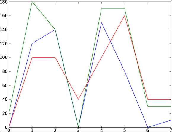
FIGURE 14-2: Time-series plot of monthly snow depth data.

Each line in the graph represents the depth of snow at different locations in the same month. The preceding code you use to build this graph is simple; if you want to make a better representation, you could add color or text font attributes to the plot function. Of course, you can also use other types of data graphics, depending on which types best show the data trends you want to display. What’s important here is that you know when to use each of these important libraries and that you understand how you can use the Python programming language to make data analysis both easy and efficient.

Learning from data with Scikit-learn

Scikit-learn is far and away Python’s best machine learning library. With it, you can execute all sorts of machine learning methods, including classification, regression, clustering, dimensionality reduction, and more. The library also offers a preprocessing module that is wonderfully supportive whenever you need to prepare your data for predictive modeling. Lastly, Scikit-learn offers a model selection module that’s readily available with all sorts of metrics to help you build your models and choose the best performing model among a selection.

Analyzing Data with Python — an Exercise

Most of Python’s recent growth has been among users from the science community, which means that most users probably didn’t study computer science in school yet find programming to be a skill they must have in order to work in their respective fields. Python’s uncomplicated, human-readable syntax and its welcoming user community have created a large and dedicated user base. The remainder of this chapter can help get you started in analyzing data using Python.

In the exercise I spell out in this section, I refer to a hypothetical classroom dataset, but I want to start out by showing you where to go to do an easy install-and-setup of a good Python programming environment. From there, I show you how to import the classroom-data CSV file into Python, how to use Python to calculate a weighted grade average for students in the class, and how to use Python to generate an average trendline of student grades.

Installing Python on the Mac and Windows OS

The Mac comes with a basic version of Python preinstalled; Windows doesn’t ship with Python. Whether you’re on the Mac or a Windows PC, I recommend downloading a free Python distribution that gives you easy access to as many useful modules as possible. I’ve tried several distributions — the one I recommend is Anaconda, by Continuum Analytics (available from https://store.continuum.io/cshop/anaconda). It comes with more than 150 Python packages, including NumPy, SciPy, Pandas, MatPlotLib, and Scikit-learn.

To do something of any magnitude in Python, you also need a programming environment. Anaconda comes with the IPython programming environment, which I recommend. IPython, which runs in Jupyter Notebooks (from directly within your web browser), allows you to write code in separate cells and then see the results for each step. To open Jupyter in your web browser after installing Anaconda, just navigate to, and open, the Jupyter Notebook program. That program automatically launches the web browser application, shown in Figure 14-3.

Source: Lynda.com, Python for DS

FIGURE 14-3: The Jupyter Notebook / IPython programming environment.

When you’re using data science to solve problems, you aren’t writing the programs yourself. Rather, you’re using prebuilt programming tools and languages to interact with your data.

When you download your free Python distribution, you have a choice between version 2 or version 3. In 2010, the Python language was completely overhauled to make it more powerful in ways that only computer scientists would understand. The problem is that the new version is not backward-compatible — in other words, Python 2 scripts aren’t compatible with a Python 3 environment. Python 2 scripts need syntax changes to run in Python 3. This sounds like a terrible situation, and though it’s not without controversy, most pythonistas (Python users) are fine with it.

I highly recommend that you use the final Python 2 release, version Python 2.7. As of late 2016, that version is still being used by the majority of Python users (caveat: except perhaps those whom hold a degree in Computer Science). It performs great for data science, it’s easier to learn than Python 3, and sites such as GitHub have millions of snippets and scripts that you can copy to make your life easier.

Loading CSV files

To load data from a comma-separated values (CSV) file, use the Pandas library. I walk you through the process in the code shown in Listing 14-2. For this exercise, you’ll need to download the class_grades.csv file from the GitHub repository for this course (at https://github.com/BigDataGal/Data-Science-for-Dummies). Before getting started, make sure to place your data file — the class_grades.csv file, to be precise — in the Jupyter Notebooks folder. By default, IPython always looks at the Jupyter Notebooks folder to find any external files that are called by your code.

Just in case you don’t know about commenting yet, in Python a coder can insert comments on the code by prefixing every comment line with the hash symbol (#). All comments are invisible to the application — they aren’t acted on — but they are visible to the programmers and their buddies (and to their enemies, for that matter).

LISTING 14-2 Sample Code for Loading a CSV File into Python

import pandas as pd
import numpy as np
import matplotlib.pyplot as plt
from scipy import stats
# This loads the modules I’ll use throughout this notebook, giving each a short alias.

%matplotlib inline
# This will show charts below each cell instead of in a separate viewer.

grades = pd.read_csv('class_grades.csv')
# That’s it, you’re done!

print grades.head()

Figure 14-4 shows you what IPython comes up with when fed this code.

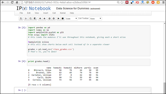
FIGURE 14-4: Using Pandas to import a CSV file into Jupyter.

If you want to limit the code output to the first five rows only, you can use the head() function.

Calculating a weighted average

Okay, so you’ve fed IPython (if you’ve read the preceding section) a lot of student grades that were stored in a CSV file. The question is, how do you want these grades calculated? In other words, how do you want to weigh each separate component of the grade?

I’m just going to make a command decision and say that final grades are to be calculated this way:

· Homework assignment 1 = 10 percent

· Homework assignment 2 = 10 percent

· Midterm = 25 percent

· Class participation = 10 percent

· Final exam = 45 percent

With Pandas, you can easily calculate each student’s weighted final grade. Listing 14-3 shows you how it’s done.

LISTING 14-3 Sample Code for Calculating a Weighted Average in Python

import pandas as pd
import numpy as np
import matplotlib.pyplot as plt
from scipy import stats
%matplotlib inline
grades = pd.read_csv('class_grades.csv')
grades['grade'] = np.round((0.1 * grades.homewk1 + 0.1 * grades.homewk2 + 0.25 * grades.midterm + 0.1 * grades.partic + 0.45 * grades.exam), 0)

# This creates a new column called 'grade' and populates it based on the values of other columns, rounded to an integer.

print grades.tail()

Figure 14-5 shows the results of your new round of coding.

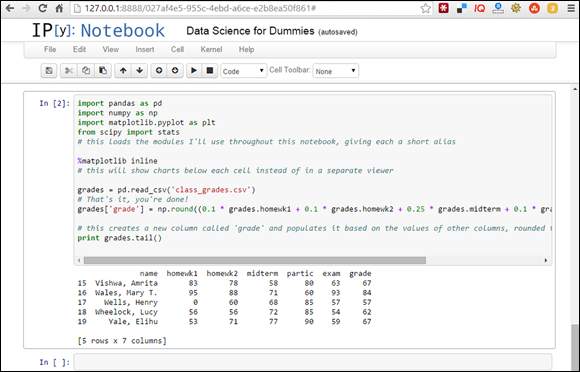
FIGURE 14-5: Calculating a weighted average in IPython.

If you want to limit your code output to the last five rows only, you can use the tail() function.

Just for fun, you can calculate letter grades with a letter_grade function and if commands. The code is shown in Listing 14-4, and the results are shown in Figure 14-6.

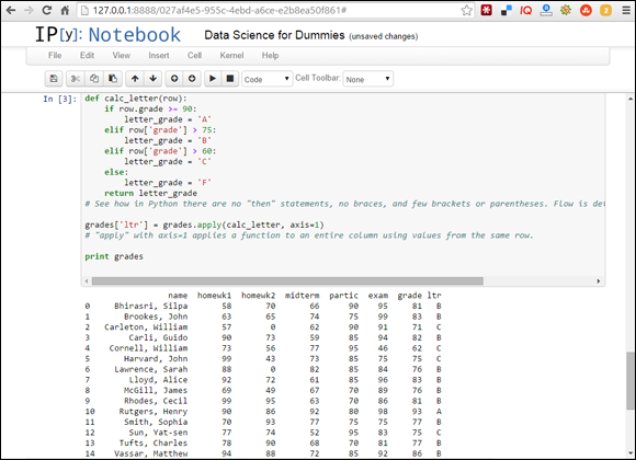
FIGURE 14-6: Calculating a weighted average using a letter_grade function and an if command.

LISTING 14-4 Using a letter_grade Function and an if Command in Python

def calc_letter(row):
if row.grade >= 90:
letter_grade = 'A'
elif row['grade'] > 75:
letter_grade = 'B'
elif row['grade'] > 60:
letter_grade = 'C'
else:
letter_grade = 'F'
return letter_grade

# See how in Python there are no “then” statements, no braces, and few brackets or parentheses. Flow is determined by colons and indents.

grades['ltr'] = grades.apply(calc_letter, axis=1)

# “apply” with axis=1 applies a function to an entire column using values from the same row.

print grades

Drawing trendlines

Using SciPy, you can easily draw a trendline — a line on a chart that indicates the overall trend of a dataset. Popular kinds of trendlines include best-fit lines, regression lines, and ordinary least squares lines. In this section, I show you how to track the progress of any student in our hypothetical class, from the beginning of the semester to the end. For this example, I’ve created a trendline for the first student, Silpa Bhirasri. You can generate a trendline for any student, however, simply by plugging that person’s name into the student variable.

To use SciPy, you first need to make a basic Python ordered list (denoted by numbers or strings in square brackets) and then turn those numbers or strings into a NumPy array. This new array allows you to run calculations on all values at one time, rather than have to write code to run over each of the values separately. Lastly, you calculate the best-fit line for y-values (the x-values are always the same as the original series) and draw the chart in the Jupyter Notebook using four lines of code from the MatPlotLib library. Listing 14-5 puts it all together for you.

LISTING 14-5 Sample Code for Creating a Trendline in Python

student = 'Bhirasri, Silpa'

y_values = [] # create an empty list
for column in ['homewk1', 'homewk2', 'midterm', 'partic', 'exam']:
y_values.append(grades[grades.name == student][column].iloc[0])
# Append each grade in the order it appears in the dataframe.
print y_values

x = np.array([1, 2, 3, 4, 5])
y = np.array(y_values)
slope, intercept, r, p, slope_std_err = stats.linregress(x, y)
# This automatically calculates the slope, intercept, Pearson correlation, coefficient (r), and two other statistics I won't use here.

bestfit_y = intercept + slope * x
# This calculates the best-fit line to show on the chart.

plt.plot(x, y, 'ko')
# This plots x and y values; 'k' is the standard printer's abbreviation for the color 'blacK', and 'o' signifies markers to be circular.
plt.plot(x, bestfit_y, 'r-')
# This plots the best fit regression line as a 'r'ed line('-').

plt.ylim(0, 100)
# This sets the upper and lower limits of the y axis.
# If it were not specified, the minimum and maximum values would be used.
plt.show() # since the plot is ready, it will be shown below the cell
print 'Pearson coefficient (R) = ' + str(r)

Figure 14-7 shows the trendline for the student named Silpa Bhirasri.

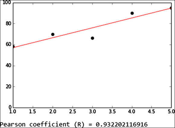
FIGURE 14-7: A trendline generated in IPython.

From the trendline shown in the figure, you can see that Silpa’s grades steadily improved all semester, except for a little dip at the midterm. At about 0.93, the Pearson correlation coefficient is high, indicating that Silpa’s grades improved, and it’s close to a linear progression. For more on the Pearson coefficient, check out Chapter 5.