Data Science For Dummies (2016)
Part 2
Using Data Science to Extract Meaning from Your Data
Chapter 5
Math, Probability, and Statistical Modeling
IN THIS CHAPTER
![]() Introducing the core basics of statistical probability
Introducing the core basics of statistical probability
![]() Quantifying correlation
Quantifying correlation
![]() Reducing dataset dimensionality
Reducing dataset dimensionality
![]() Building decision models with multi-criteria decision making
Building decision models with multi-criteria decision making
![]() Diving into regression methods
Diving into regression methods
![]() Overviewing outlier detection
Overviewing outlier detection
![]() Talking about time series analysis
Talking about time series analysis
Math and statistics are not the scary monsters that many people make them out to be. In data science, the need for these quantitative methods is simply a fact of life — and nothing to get alarmed over. Although you must have a handle on the math and statistics that are necessary to solve a problem, you don’t need to go study and get a degree in those fields.
Contrary to what many pure statisticians would have you believe, the data science field is not the same as the statistics field. Data scientists have substantive knowledge in one field or several fields, and they use statistics, math, coding, and strong communication skills to help them discover, understand, and communicate data insights that lie within raw datasets related to their field of expertise. Statistics is a vital component of this formula, but not more vital than the others. In this chapter, I introduce you to the basic ideas behind probability, correlation analysis, dimensionality reduction, decision modeling, regression analysis, outlier detection, and time series analysis.
Exploring Probability and Inferential Statistics
Probability is one of the most fundamental concepts in statistics. To even get started in making sense of your data by using statistics, you need to be able to identify something as basic as whether you’re looking at descriptive or inferential statistics. You also need a firm grasp of the basics of probability distribution. The following sections cover these concepts and more.
A statistic is a result that’s derived from performing a mathematical operation on numerical data. In general, you use statistics in decision making. Statistics come in two flavors:
· Descriptive: Descriptive statistics provide a description that illuminates some characteristic of a numerical dataset, including dataset distribution, central tendency (such as mean, min, or max), and dispersion (as in standard deviation and variance).
· Inferential: Rather than focus on pertinent descriptions of a dataset, inferential statistics carve out a smaller section of the dataset and attempt to deduce significant information about the larger dataset. Use this type of statistics to get information about a real-world measure in which you’re interested.
It’s true that descriptive statistics describe the characteristics of a numerical dataset, but that doesn’t tell you why you should care. In fact, most data scientists are interested in descriptive statistics only because of what they reveal about the real-world measures they describe. For example, a descriptive statistic is often associated with a degree of accuracy, indicating the statistic’s value as an estimate of the real-world measure.
To better understand this concept, imagine that a business owner wants to estimate the upcoming quarter’s profits. The owner might take an average of the past few quarters’ profits to use as an estimate of how much he’ll make during the next quarter. But if the previous quarters’ profits varied widely, a descriptive statistic that estimated the variation of this predicted profit value (the amount by which this dollar estimate could differ from the actual profits he will make) would indicate just how far off the predicted value could be from the actual one. (Not bad information to have, right?)
 You can use descriptive statistics in many ways — to detect outliers, for example, or to plan for feature preprocessing requirements or to quickly identify what features you may want, or not want, to use in an analysis.
Like descriptive statistics, inferential statistics are used to reveal something about a real-world measure. Inferential statistics do this by providing information about a small data selection, so you can use this information to infer something about the larger dataset from which it was taken. In statistics, this smaller data selection is known as a sample, and the larger, complete dataset from which the sample is taken is called the population.
If your dataset is too big to analyze in its entirety, pull a smaller sample of this dataset, analyze it, and then make inferences about the entire dataset based on what you learn from analyzing the sample. You can also use inferential statistics in situations where you simply can’t afford to collect data for the entire population. In this case, you’d use the data you do have to make inferences about the population at large. At other times, you may find yourself in situations where complete information for the population is not available. In these cases, you can use inferential statistics to estimate values for the missing data based on what you learn from analyzing the data that is available.
 For an inference to be valid, you must select your sample carefully so that you get a true representation of the population. Even if your sample is representative, the numbers in the sample dataset will always exhibit some noise — random variation, in other words — that guarantees the sample statistic is not exactly identical to its corresponding population statistic.
Probability distributions
Imagine that you’ve just rolled into Las Vegas and settled into your favorite roulette table over at the Bellagio. When the roulette wheel spins off, you intuitively understand that there is an equal chance that the ball will fall into any of the slots of the cylinder on the wheel. The slot where the ball will land is totally random, and the probability, or likelihood, of the ball landing in any one slot over another is the same. Because the ball can land in any slot, with equal probability, there is an equal probability distribution, or a uniform probability distribution — the ball has an equal probability of landing in any of the slots in the cylinder.
But the slots of the roulette wheel are not all the same — the wheel has 18 black slots and 20 slots that are either red or green. Because of this arrangement, there is 18/38 probability that your ball will land on a black slot. You plan to make successive bets that the ball will land on a black slot.
Your net winnings here can be considered a random variable, which is a measure of a trait or value associated with an object, a person, or a place (something in the real world) that is unpredictable. Because this trait or value is unpredictable, however, doesn’t mean that you know nothing about it. What’s more, you can use what you do know about this thing to help you in your decision making. Here’s how …
A weighted average is an average value of a measure over a very large number of data points. If you take a weighted average of your winnings (your random variable) across the probability distribution, this would yield an expectation value — an expected value for your net winnings over a successive number of bets. (An expectation can also be thought of as the best guess, if you had to guess.) To describe it more formally, an expectation is a weighted average of some measure associated with a random variable. If your goal is to model an unpredictable variable so that you can make data-informed decisions based on what you know about its probability in a population, you can use random variables and probability distributions to do this.
 When considering the probability of an event, you must know what other events are possible. Always define the set of events as mutually exclusive — only one can occur at a time. (Think of the six possible results of rolling a die.) Probability has these two important characteristics:
· The probability of any single event never goes below 0.0 or exceeds 1.0.
· The probability of all events always sums to exactly 1.0.
Probability distribution is classified per these two types:
· Discrete: A random variable where values can be counted by groupings
· Continuous: A random variable that assigns probabilities to a range of value
To understand discrete and continuous distribution, think of two variables from a dataset describing cars. A “color” variable would have a discrete distribution because cars have only a limited range of colors (black, red, or blue, for example). The observations would be countable per the color grouping. A variable describing cars’ miles per gallon, or “mpg,” would have a continuous distribution because each car could have its own separate value for “mpg.”
· Normal distributions (numeric continuous): Represented graphically by a symmetric bell-shaped curve, these distributions model phenomena that tend toward some most-likely observation (at the top of the bell in the bell curve); observations at the two extremes are less likely.
· Binomial distributions (numeric discrete): Model the number of successes that can occur in a certain number of attempts when only two outcomes are possible (the old heads-or-tails coin flip scenario, for example). Binaryvariables — variables that assume only one of two values — have a binomial distribution.
· Categorical distributions (non-numeric): Represents either non-numeric categorical variables or ordinal variables (a special case of numeric variable that can be grouped and ranked like a categorical variable).
Conditional probability with Naïve Bayes
You can use the Naïve Bayes machine learning method, which was borrowed straight from the statistics field, to predict the likelihood that an event will occur, given evidence defined in your data features — something called conditional probability. Naïve Bayes, which is based on classification and regression, is especially useful if you need to classify text data.
To better illustrate this concept, consider the Spambase dataset that’s available from UCI’s machine learning repository (https://archive.ics.uci.edu/ml/datasets/Spambase). That dataset contains 4,601 records of emails and, in its last field, designates whether each email is spam. From this dataset, you can identify common characteristics between spam emails. Once you’ve defined common features that indicate spam email, you can build a Naïve Bayes classifier that reliably predicts whether an incoming email is spam, based on the empirical evidence supported in its content. In other words, the model predicts whether an email is spam — the event — based on features gathered from its content — the evidence.
Naïve Bayes comes in these three popular flavors:
· MultinomialNB: Use this version if your variables (categorical or continuous) describe discrete frequency counts, like word counts. This version of Naïve Bayes assumes a multinomial distribution, as is often the case with text data. It does not except negative values.
· BernoulliNB: If your features are binary, you use multinomial Bernoulli Naïve Bayes to make predictions. This version works for classifying text data, but isn’t generally known to perform as well as MultinomialNB. If you want to use BernoulliNB to make predictions from continuous variables, that will work, but you first need to sub-divide them into discrete interval groupings (also known as binning).
· GaussianNB: Use this version if all predictive features are normally distributed. It’s not a good option for classifying text data, but it can be a good choice if your data contains both positive and negative values (and if your features have a normal distribution, of course).
Before building a Bayes classifier naїvely, consider that the model holds an a priori assumption. Its predictions assume that past conditions still hold true. Predicting future values from historical ones generates incorrect results when present circumstances change.
Quantifying Correlation
Many statistical and machine learning methods assume that your features are independent. To test whether they’re independent, though, you need to evaluate their correlation — the extent to which variables demonstrate interdependency. In this section, you get a brief introduction to Pearson correlation and Spearman’s rank correlation.
Correlation is quantified per the value of a variable called r, which ranges between -1 and 1. The closer the r-value is to 1 or -1, the more correlation there is between two variables. If two variables have an r-value that’s close to 0, it could indicate that they’re independent variables.
Calculating correlation with Pearson’s r
If you want to uncover dependent relationships between continuous variables in a dataset, you’d use statistics to estimate their correlation. The simplest form of correlation analysis is the Pearson correlation, which assumes that
· Your data is normally distributed.
· You have continuous, numeric variables.
· Your variables are linearly related.
Because the Pearson correlation has so many conditions, only use it to determine whether a relationship between two variables exists, but not to rule out possible relationships. If you were to get an r-value that is close to 0, it indicates that there is no linear relationship between the variables, but that a nonlinear relationship between them still could exist.
Ranking variable-pairs using Spearman’s rank correlation
The Spearman’s rank correlation is a popular test for determining correlation between ordinal variables. By applying Spearman’s rank correlation, you’re converting numeric variable-pairs into ranks by calculating the strength of the relationship between variables and then ranking them per their correlation.
The Spearman’s rank correlation assumes that
· Your variables are ordinal.
· Your variables are related non-linearly.
· Your data is non-normally distributed.
Reducing Data Dimensionality with Linear Algebra
Any intermediate-level data scientist should have a pretty good understanding of linear algebra and how to do math using matrices. Array and matrix objects are the primary data structure in analytical computing. You need them in order to perform mathematical and statistical operations on large and multidimensional datasets — datasets with many different features to be tracked simultaneously. In this section, you see exactly what is involved in using linear algebra and machine learning methods to reduce a dataset’s dimensionality.
Decomposing data to reduce dimensionality
To start at the very beginning, you need to understand the concept of eigenvector. To conceptualize an eigenvector, think of a matrix called A. Now consider a non-zero vector called x and that Ax = λx for a scalar λ. In this scenario, scalar λ is what’s called an eigenvalue of matrix A. It’s permitted to take on a value of 0. Furthermore, x is the eigenvector that corresponds to λ, and again, it’s not permitted to be a zero value.
Okay, so what can you do with all this theory? Well, for starters, using a linear algebra method called singular value decomposition (SVD), you can reduce the dimensionality of your dataset — or the number of features that you track when carrying out an analysis. Dimension reduction algorithms are ideal options if you need to compress your dataset while also removing redundant information and noise.
The SVD linear algebra method decomposes the data matrix into the three resultant matrices shown in Figure 5-1. The product of these matrices, when multiplied together, gives you back your original matrix. SVD is handy when you want to remove redundant information by compressing your dataset.

FIGURE 5-1: You can use SVD to decompose data down to u, S, and V matrices.
Take a closer look at the figure:
A = u * v * S
· A: This is the matrix that holds all your original data.
· u: This is a left-singular vector (an eigenvector) of A, and it holds all the important, non-redundant information about your data’s observations.
· v: This is a right-singular eigenvector of A. It holds all the important, non-redundant information about columns in your dataset’s features.
· S: This is the square root of the eigenvalue of A. It contains all the information about the procedures performed during the compression.
Although it might sound complicated, it’s pretty simple. Imagine that you’ve compressed your dataset and it has resulted in a matrix S that sums to 100. If the first value in S is 97 and the second value is 94, this means that the first two columns contain 94 percent of the dataset’s information. In other words, the first two columns of the u matrix and the first two rows of the v matrix contain 94 percent of the important information held in your original dataset, A. To isolate only the important, non-redundant information, you’d keep only those two columns and discard the rest.
When you go to reconstruct your matrix by taking the dot product of S, u, and v, you'll probably notice that the resulting matrix is not an exact match to your original dataset. Worry not! That's the data that remains after much of the information redundancy and noise has been filtered out by SVD.
When deciding the number of rows and columns to keep, it’s okay to get rid of rows and columns, as long as you make sure that you retain at least 70 percent of the dataset's original information.
Reducing dimensionality with factor analysis
Factor analysis is along the same lines as SVD in that it’s a method you can use for filtering out redundant information and noise from your data. An offspring of the psychometrics field, this method was developed to help you derive a root cause, in cases where a shared root cause results in shared variance — when a variable’s variance correlates with the variance of other variables in the dataset.
 A variables variability measures how much variance it has around its mean. The greater a variable’s variance, the more information that variable contains.
When you find shared variance in your dataset, that means information redundancy is at play. You can use factor analysis or principal component analysis to clear your data of this information redundancy. You see more on principal component analysis in the following section, but for now, focus on factor analysis and the fact that you can use it to compress your dataset’s information into a reduced set of meaningful, non-information-redundant latent variables — meaningful inferred variables that underlie a dataset but are not directly observable.
Factor analysis makes the following assumptions:
· Your features are metric — numeric variables on which meaningful calculations can be made.
· Your features should be continuous or ordinal.
· You have more than 100 observations in your dataset and at least 5 observations per feature.
· Your sample is homogenous.
· There is r > 0.3 correlation between the features in your dataset.
In factor analysis, you do a regression on features to uncover underlying latent variables, or factors. You can then use those factors as variables in future analyses, to represent the original dataset from which they’re derived. At its core, factor analysis is the process of fitting a model to prepare a dataset for analysis by reducing its dimensionality and information redundancy.
Decreasing dimensionality and removing outliers with PCA
Principal component analysis (PCA) is another dimensionality reduction technique that’s closely related to SVD: This unsupervised statistical method finds relationships between features in your dataset and then transforms and reduces them to a set of non-information-redundant principle components — uncorrelated features that embody and explain the information that’s contained within the dataset (that is, its variance). These components act as a synthetic, refined representation of the dataset, with the information redundancy, noise, and outliers stripped out. You can then take those reduced components and use them as input for your machine learning algorithms, to make predictions based on a compressed representation of your data.
The PCA model makes these two assumptions:
· Multivariate normality is desirable, but not required.
· Variables in the dataset should be continuous.
Although PCA is like factor analysis, there are two major differences: One difference is that PCA does not regress to find some underlying cause of shared variance, but instead decomposes a dataset to succinctly represent its most important information in a reduced number of features. The other key difference is that, with PCA, the first time you run the model, you don’t specify the number of components to be discovered in the dataset. You let the initial model results tell you how many components to keep, and then you rerun the analysis to extract those features.
A small amount of information from your original dataset will not be captured by the principal components. Just keep the components that capture at least 95 percent of the dataset’s total variance. The remaining components won’t be that useful, so you can get rid of them.
When using PCA for outlier detection, simply plot the principal components on an x-y scatter plot and visually inspect for areas that might have outliers. Those data points correspond to potential outliers that are worth investigating.
Modeling Decisions with Multi-Criteria Decision Making
Life is complicated. We’re often forced to make decisions where several different criteria come into play, and it often seems unclear what criterion should have priority. Mathematicians, being mathematicians, have come up with quantitative approaches that you can use for decision support when you have several criteria or alternatives on which to base your decision. You see that in Chapter 4, where I talk about neural networks and deep learning, but another method that fulfills this same decision-support purpose is multi-criteria decision making (MCDM, for short).
Turning to traditional MCDM
You can use MCDM methods in anything from stock portfolio management to fashion-trend evaluation, from disease outbreak control to land development decision making. Anywhere you have two or more criteria on which you need to base your decision, you can use MCDM methods to help you evaluate alternatives.
To use multi-criteria decision making, the following two assumptions must be satisfied:
· Multi-criteria evaluation: You must have more than one criterion to optimize.
· Zero-sum system: Optimizing with respect to one criterion must come at the sacrifice of at least one other criterion. This means that there must be trade-offs between criteria — to gain with respect to one means losing with respect to at least one other.
The best way to get a solid grasp on MCDM is to see how it’s used to solve a real-world problem. MCDM is commonly used in investment portfolio theory. Pricing of individual financial instruments typically reflects the level of risk you incur, but an entire portfolio can be a mixture of virtually riskless investments (U.S. government bonds, for example) and minimum-, moderate-, and high-risk investments. Your level of risk aversion dictates the general character of your investment portfolio. Highly risk-averse investors seek safer and less lucrative investments, and less risk-averse investors choose riskier investments. In the process of evaluating the risk of a potential investment, you’d likely consider the following criteria:
· Earnings growth potential: Here, an investment that falls under an earnings growth potential threshold gets scored as a 0; anything above that threshold gets a 1.
· Earnings quality rating: If an investment falls within a ratings class for earnings quality, it gets scored as a 0; otherwise, it gets scored as a 1.
For you non-Wall Street types out there, earnings quality refers to various measures used to determine how kosher a company’s reported earnings are; such measures attempt to answer the question, “Do these reported figures pass the smell test?”
· Dividend performance: When an investment doesn’t reach a set dividend performance threshold, it gets a 0; if it reaches or surpasses that threshold, it gets a 1.
In mathematics, a set is a group of numbers that shares some similar characteristic. In traditional set theory, membership is binary — in other words, an individual is either a member of a set or it’s not. If the individual is a member, it is represented with the number 1. If it is not a member, it is represented by the number 0. Traditional MCDM is characterized by binary membership.
Imagine that you’re evaluating 20 different potential investments. In this evaluation, you’d score each criterion for each of the investments. To eliminate poor investment choices, simply sum the criteria scores for each of the alternatives and then dismiss any investments that do not get a total score of 3 — leaving you with the investments that fall within a certain threshold of earning growth potential, that have good earnings quality, and whose dividends perform at a level that’s acceptable to you.
Focusing on fuzzy MCDM
If you prefer to evaluate suitability within a range, instead of using binary membership terms of 0 or 1, you can use fuzzy multi-criteria decision making (FMCDM) to do that. With FMCDM you can evaluate all the same types of problems as you would with MCDM. The term fuzzy refers to the fact that the criteria being used to evaluate alternatives offer a range of acceptability — instead of the binary, crisp set criteria associated with traditional MCDM. Evaluations based on fuzzy criteria lead to a range of potential outcomes, each with its own level of suitability as a solution.
One important feature of FMCDM: You’re likely to have a list of several fuzzy criteria, but these criteria might not all hold the same importance in your evaluation. To correct for this, simply assign weights to criteria to quantify their relative importance.
Introducing Regression Methods
Machine learning algorithms of the regression variety were adopted from the statistics field, to provide data scientists with a set of methods for describing and quantifying the relationships between variables in a dataset. Use regression techniques if you want to determine the strength of correlation between variables in your data. You can use regression to predict future values from historical values, but be careful: Regression methods assume a cause-and-effect relationship between variables, but present circumstances are always subject to flux. Predicting future values from historical ones will generate incorrect results when present circumstances change. In this section, I tell you all about linear regression, logistic regression, and the ordinary least squares method.
Linear regression
Linear regression is a machine learning method you can use to describe and quantify the relationship between your target variable, y — the predictant, in statistics lingo — and the dataset features you’ve chosen to use as predictor variables (commonly designated as dataset X in machine learning). When you use just one variable as your predictor, linear regression is as simple as the middle school algebra formula y=mx+b. But you can also use linear regression to quantify correlations between several variables in a dataset — called multiple linear regression. Before getting too excited about using linear regression, though, make sure you’ve considered its limitations:
· Linear regression only works with numerical variables, not categorical ones.
· If your dataset has missing values, it will cause problems. Be sure to address your missing values before attempting to build a linear regression model.
· If your data has outliers present, your model will produce inaccurate results. Check for outliers before proceeding.
· The linear regression assumes that there is a linear relationship between dataset features and the target variable. Test to make sure this is the case, and if it’s not, try using a log transformation to compensate.
· The linear regression model assumes that all features are independent of each other.
· Prediction errors, or residuals, should be normally distributed.
Don’t forget dataset size! A good rule of thumb is that you should have at least 20 observations per predictive feature if you expect to generate reliable results using linear regression.
Logistic regression
Logistic regression is a machine learning method you can use to estimate values for a categorical target variable based on your selected features. Your target variable should be numeric, and contain values that describe the target’s class — or category. One cool thing about logistic regression is that, in addition to predicting the class of observations in your target variable, it indicates the probability for each of its estimates. Though logistic regression is like linear regression, it’s requirements are simpler, in that:
· There does not need to be a linear relationship between the features and target variable.
· Residuals don’t have to be normally distributed.
· Predictive features are not required to have a normal distribution.
When deciding whether logistic regression is a good choice for you, make sure to consider the following limitations:
· Missing values should be treated or removed.
· Your target variable must be binary or ordinal.
· Predictive features should be independent of each other.
Logistic regression requires a greater number of observations (than linear regression) to produce a reliable result. The rule of thumb is that you should have at least 50 observations per predictive feature if you expect to generate reliable results.
Ordinary least squares (OLS) regression methods
Ordinary least squares (OLS) is a statistical method that fits a linear regression line to a dataset. With OLS, you do this by squaring the vertical distance values that describe the distances between the data points and the best-fit line, adding up those squared distances, and then adjusting the placement of the best-fit line so that the summed squared distance value is minimized. Use OLS if you want to construct a function that’s a close approximation to your data.
As always, don’t expect the actual value to be identical to the value predicted by the regression. Values predicted by the regression are simply estimates that are most similar to the actual values in the model.
OLS is particularly useful for fitting a regression line to models containing more than one independent variable. In this way, you can use OLS to estimate the target from dataset features.
When using OLS regression methods to fit a regression line that has more than one independent variable, two or more of the IVs may be interrelated. When two or more IVs are strongly correlated with each other, this is called multicollinearity. Multicollinearity tends to adversely affect the reliability of the IVs as predictors when they’re examined apart from one another. Luckily, however, multicollinearity doesn’t decrease the overall predictive reliability of the model when it’s considered collectively.
Detecting Outliers
Many statistical and machine learning approaches assume that there are no outliers in your data. Outlier removal is an important part of preparing your data for analysis. In this section, you see a variety of methods you can use to discover outliers in your data.
Analyzing extreme values
Outliers are data points with values that are significantly different than the majority of data points comprising a variable. It is important to find and remove outliers, because, left untreated, they skew variable distribution, make variance appear falsely high, and cause a misrepresentation of intervariable correlations.
Most machine learning and statistical models assume that your data is free of outliers, so spotting and removing them is a critical part of preparing your data for analysis. Not only that, you can use outlier detection to spot anomalies that represent fraud, equipment failure, or cybersecurity attacks. In other words, outlier detection is a data preparation method and an analytical method in its own right.
Outliers fall into the following three categories:
· Point: Point outliers are data points with anomalous values compared to the normal range of values in a feature.
· Contextual: Contextual outliers are data points that are anomalous only within a specific context. To illustrate, if you are inspecting weather station data from January in Orlando, Florida, and you see a temperature reading of 23 degrees F, this would be quite anomalous because the average temperature there is 70 degrees F in January. But consider if you were looking at data from January at a weather station in Anchorage, Alaska — a temperature reading of 23 degrees F in this context is not anomalous at all.
· Collective: These outliers appear nearby to one another, all having similar values that are anomalous to the majority of values in the feature.
You can detect outliers using either a univariate or multivariate approach.
Detecting outliers with univariate analysis
Univariate outlier detection is where you look at features in your dataset, and inspect them individually for anomalous values. There are two simple methods for doing this:
· Tukey outlier labeling
· Tukey boxplot
It is cumbersome to detect outliers using Tukey outlier labeling, but if you want to do it, the trick here is to see how far the minimum and maximum values are from the 25 and 75 percentiles. The distance between the 1st quartile(at 25 percent) and the 3rd quartile (at 75 percent) is called the inter-quartile range (IQR), and it describes the data’s spread. When you look at a variable, consider its spread, its Q1 / Q3 values, and its minimum and maximum values to decide whether the variable is suspect for outliers.
Here’s a good rule of thumb: a = Q1 - 1.5*IQR and b = Q3 + 1.5*IQR. If your minimum value is less than a, or your maximum value is greater than b, the variable probably has outliers.
In comparison, a Tukey boxplot is a pretty easy way to spot outliers. Each boxplot has whiskers that are set at 1.5*IQR. Any values that lie beyond these whiskers are outliers. Figure 5-2 shows outliers as they appear within a Tukey boxplot.
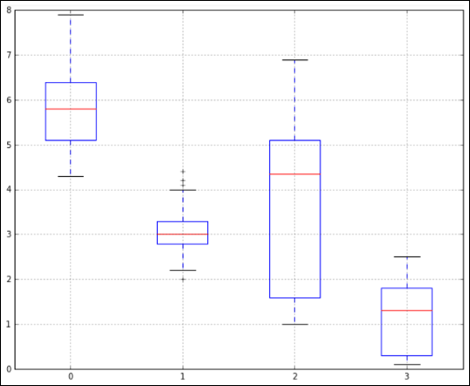
Credit: Python for DS, Lynda.com
FIGURE 5-2: Spotting outliers with a Tukey boxplot.
Detecting outliers with multivariate analysis
Sometimes outliers only show up within combinations of data points from disparate variables. These outliers really wreak havoc on machine learning algorithms, so it’s important to detect and remove them. You can use multivariate analysis of outliers to do this. A multivariate approach to outlier detection involves considering two or more variables at a time and inspecting them together for outliers. There are several methods you can use, including
· Scatter-plot matrix
· Boxplot
· Density-based spatial clustering of applications with noise (DBScan) — as discussed in Chapter 6
· Principal component analysis (shown in Figure 5-3)
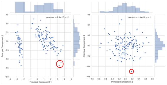
Credit: Python for DS, Lynda.com
FIGURE 5-3: Using PCA to spot outliers.
Introducing Time Series Analysis
A time series is just a collection of data on attribute values over time. Time series analysis is performed to predict future instances of the measure based on the past observational data. To forecast or predict future values from data in your dataset, use time series techniques.
Identifying patterns in time series
Time series exhibit specific patterns. Take a look at Figure 5-4 to get a better understanding of what these patterns are all about. Constant time series remain at roughly the same level over time, but are subject to some random error. In contrast, trended series show a stable linear movement up or down. Whether constant or trended, time series may also sometimes exhibit seasonality — predictable, cyclical fluctuations that reoccur seasonally throughout a year. As an example of seasonal time series, consider how many businesses show increased sales during the holiday season.

FIGURE 5-4: A comparison of patterns exhibited by time series.
If you’re including seasonality in your model, incorporate it in the quarter, month, or even 6-month period — wherever it’s appropriate. Time series may show nonstationary processes — or, unpredictable cyclical behavior that is not related to seasonality and that results from economic or industry-wide conditions instead. Because they’re not predictable, nonstationary processes can’t be forecasted. You must transform nonstationary data to stationary data before moving forward with an evaluation.
Take a look at the solid lines in Figure 5-4. These represent the mathematical models used to forecast points in the time series. The mathematical models shown represent very good, precise forecasts because they’re a very close fit to the actual data. The actual data contains some random error, thus making it impossible to forecast perfectly.
Modeling univariate time series data
Similar to how multivariate analysis is the analysis of relationships between multiple variables, univariate analysis is the quantitative analysis of only one variable at a time. When you model univariate time series, you are modeling time series changes that represent changes in a single variable over time.
Autoregressive moving average (ARMA) is a class of forecasting methods that you can use to predict future values from current and historical data. As its name implies, the family of ARMA models combines autoregressiontechniques (analyses that assume that previous observations are good predictors of future values and perform an autoregression analysis to forecast for those future values) and moving average techniques — models that measure the level of the constant time series and then update the forecast model if any changes are detected. If you’re looking for a simple model or a model that will work for only a small dataset, the ARMA model is not a good fit for your needs. An alternative in this case might be to just stick with simple linear regression. In Figure 5-5, you can see that the model forecast data and the actual data are a very close fit.

FIGURE 5-5: An example of an ARMA forecast model.
To use the ARMA model for reliable results, you need to have at least 50 observations.
All materials on the site are licensed Creative Commons Attribution-Sharealike 3.0 Unported CC BY-SA 3.0 & GNU Free Documentation License (GFDL)
If you are the copyright holder of any material contained on our site and intend to remove it, please contact our site administrator for approval.
© 2016-2026 All site design rights belong to S.Y.A.