ElasticSearch Cookbook, Second Edition (2015)
Chapter 6. Aggregations
In this chapter, we will cover the following topics:
· Executing an aggregation
· Executing the stats aggregation
· Executing the terms aggregation
· Executing the range aggregation
· Executing the histogram aggregation
· Executing the date histogram aggregation
· Executing the filter aggregation
· Executing the global aggregation
· Executing the geo distance aggregation
· Executing the nested aggregation
· Executing the top hit aggregation
Introduction
In developing search solutions, not only are results important, but they also help us to improve quality and search focus.
ElasticSearch provides a powerful tool to achieve these goals: aggregations.
The main usage of aggregations is to provide additional data to the search results to improve their quality or to augment them with additional information. For example, in searching for news articles, facets that can be interesting for calculation are the articles written by authors and the date histogram of their publishing date.
Thus, aggregations are used not only to improve results, but also to provide an insight into stored data (Analytics); for this, we have a lot of tools, and one of which is called Kibana (http://www.elasticsearch.org/overview/kibana/).
Generally, the aggregations are displayed to the end user with graphs or a group of filtering options (for example, a list of categories for the search results).
The actual aggregation framework is an evolution of the previous ElasticSearch functionality called facets. Facets were helpful and powerful, but had a lot of limitations in their design. The ElasticSearch team decided to evolve them into the aggregation framework (facets are already deprecated in ElasticSearch 1.x, and they will be removed from the next ElasticSearch major release also). For a complete coverage of facets, take a look at ElasticSearch Cookbook, Packt Publishing, at http://www.packtpub.com/elasticsearch-cookbook/book.
Since the ElasticSearch aggregation framework provides scripting functionalities, it is able to cover a wide spectrum of scenarios. In this chapter, some simple scripting functionalities are shown related to aggregations, but we will cover in-depth scripting in the next chapter.
The aggregation framework is also the base for advanced analytics as shown in software such as Kibana (http://www.elasticsearch.org/overview/kibana/), or similar software. It's very important to understand how the various types of aggregations work and when to choose them.
Executing an aggregation
ElasticSearch provides several functionalities other than search; it allows executing statistics and real-time analytics on searches via aggregations.
Getting ready
You need a working ElasticSearch cluster and an index populated with the script, which is available at https://github.com/aparo/elasticsearch-cookbook-second-edition.
How to do it...
To execute an aggregation, we will perform the steps given as follows:
1. From the command line, we can execute a query with aggregations:
2. curl -XGET 'http://127.0.0.1:9200/test-index/test-type/_search?pretty=true&size=0' -d '{
3. "query": {
4. "match_all": {}
5. },
6. "aggregations": {
7. "tag": {
8. "terms": {
9. "field": "tag",
10. "size": 10
11. }
12. }
13. }
14.}'
In this case, we have used a match_all query plus a terms aggregation that is used to count terms.
15. The result returned by ElasticSearch, if everything is all right, should be:
16.{
17. "took" : 3,
18. "timed_out" : false,
19. "_shards" : {… truncated …},
20. "hits" : {
21. "total" : 1000,
22. "max_score" : 0.0,
23. "hits" : [ ]
24. },
25. "aggregations" : {
26. "tag" : {
27. "buckets" : [ {
28. "key" : "laborum",
29. "doc_count" : 25
30. }, {
31. "key" : "quidem",
32. "doc_count" : 15
33. }, {
34. "key" : "maiores",
35. "doc_count" : 14
36. }, {
37.…. Truncated ….
38. }, {
39. "key" : "praesentium",
40. "doc_count" : 9
41. } ]
42. }
43. }
}
The results are not returned because we have fixed the result size to 0. The aggregation result is contained in the aggregation field. Each type of aggregation has its own result format (the explanation of this kind of result is in the Executing terms aggregationrecipe in this chapter).
Tip
It's possible to execute an aggregation calculation without returning search results to reduce bandwidth by passing the search size parameter set to 0.
How it works...
Every search can return an aggregation calculation, computed on the query results; the aggregation phase is an additional step in query postprocessing—for example, highlighting the results. To activate the aggregation phase, an aggregation must be defined using the aggs or aggregations keyword.
There are several types of aggregation that can be used in ElasticSearch.
In this chapter, we'll cover all standard aggregations available; additional aggregation types can be provided with a plugin and scripting.
Aggregations are the bases for real-time analytics. They allow us to execute:
· Counting
· Histograms
· The range aggregation
· Statistics
· The geo distance aggregation
The following shows the executed query results using a histogram:
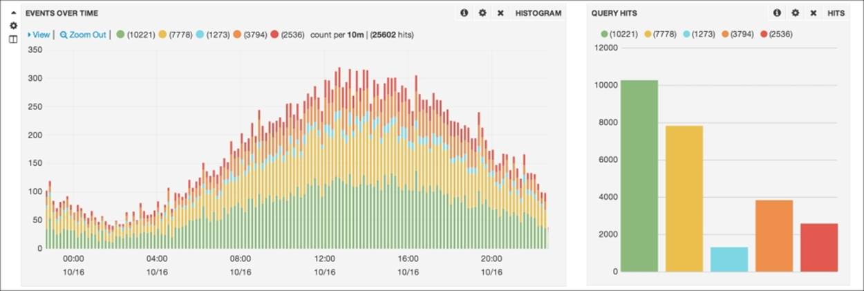
Aggregations are always executed on search hits; they are usually computed in a Map/Reduce way. The map step is distributed in shards, but the reduce step is done in the called node.
As aggregation computation requires a lot of data to be kept in memory; it can be very memory-intensive. For example, to execute a terms aggregation, it requires that all unique terms in the field, which is used for aggregating, be kept in memory. Executing this operation on million of documents requires storing a large number of values in memory.
The aggregation framework was introduced in ElasticSearch 1.x as an evolution of the facets feature. Its main difference from facets is the possibility of executing the analytics with several nesting levels of subaggregations; facets were plain and were limited to a single-level aggregation. Aggregations keep information of documents that go into an aggregation bucket, and an aggregation output can be the input of the next aggregation.
Tip
Aggregations can be composed in a complex tree of subaggregations without depth limits.
The generic form for an aggregation is as follows:
"aggregations" : {
"<aggregation_name>" : {
"<aggregation_type>" : {
<aggregation_body>
}
[,"aggregations" : { [<sub_aggregation>]+ } ]?
}
[,"<aggregation_name_2>" : { ... } ]*
}
Aggregation nesting allows us to cover very advanced scenarios in executing analytics such as aggregating data by country, by region, or by people's ages, where age groups are ordered in the descending order. There are no more limits in mastering analytics.
The following schema summarizes the main difference between the deprecated facets system and the aggregation framework:
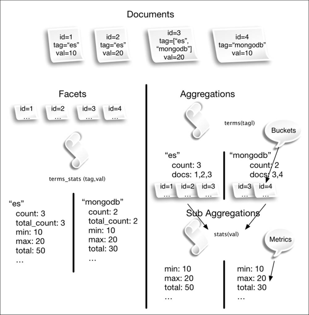
As you can see in the preceding figure, there are two kinds of aggregators:
· Bucketing aggregators: They produce buckets, where a bucket has an associated value and a set of documents (for example, the terms aggregator produces a bucket per term for the field it's aggregating on). A document can end up in multiple buckets if the document has multiple values for the field being aggregated on (in our example, the document with id=3). If a bucket aggregator has one or more downstream (such as, child) aggregators, these are run on each generated bucket.
· Metric aggregators: They receive a set of documents as input and produce statistical results computed for the specified field. The output of metric aggregators does not include any information linked to individual documents; it contains just the statistical data.
Generally, the order of buckets depends on the bucket aggregator used—for example, when using the terms aggregator, the buckets are, by default, ordered by count. The aggregation framework allows us to order by subaggregation metrics (for example, the preceding example can be ordered by the stats.avg value).
See also
· Refer to the Executing the terms aggregation recipe in this chapter for a more detailed explanation of aggregation
Executing the stats aggregation
The most commonly used metric aggregations are stats aggregations. They are generally used as terminal aggregation steps to compute a value to be used directly or for sorting.
Getting ready
You need a working ElasticSearch cluster and an index populated with the script (chapter_06/executing_stat_aggregations.sh) available at https://github.com/aparo/elasticsearch-cookbook-second-edition.
How to do it...
To execute a stats aggregation, we will perform the steps given as follows:
1. We want to calculate all statistical values of a matched query in the age field. The REST call should be as follows:
2. curl -XPOST "http://127.0.0.1:9200/test-index/_search?size=0" -d '
3. {
4. "query": {
5. "match_all": {}
6. },
7. "aggs": {
8. "age_stats": {
9. "extended_stats": {
10. "field": "age"
11. }
12. }
13. }
14.}'
15. The result, if everything is fine, should be:
16.{
17. "took" : 2,
18. "timed_out" : false,
19. "_shards" : { …truncated…},
20. "hits" : {
21. "total" : 1000,
22. "max_score" : 0.0,
23. "hits" : [ ]
24. },
25. "aggregations" : {
26. "age_stats" : {
27. "count" : 1000,
28. "min" : 1.0,
29. "max" : 100.0,
30. "avg" : 53.243,
31. "sum" : 53243.0,
32. "sum_of_squares" : 3653701.0,
33. "variance" : 818.8839509999999,
34. "std_deviation" : 28.616148430562767
35. }
36. }
}
In the answer, under the aggregations field, we have the statistical results of our aggregation under the defined field age_stats.
How it works...
After the search phase, if any aggregations are defined, they are computed.
In this case, we have requested an extended_stats aggregation labeled age_stats and that computes a lot of statistical indicators.
The available statistical aggregators are:
· min: This computes the minimum value for a group of buckets.
· max: This computes the maximum value for a group of buckets.
· avg: This computes the average value for a group of buckets.
· sum: This computes the sum of all buckets.
· value_count: This computes the count of values in the bucket.
· stats: This computes all the base metrics such as min, max, avg, count, and sum.
· extended_stats: This computes the stats metric plus variance, the standard deviation (std_deviation), and the sum of squares (sum_of_squares).
· percentiles: This computes percentiles (the point at which a certain percentage of observed values occurs) of some values. (Visit Wikipedia at http://en.wikipedia.org/wiki/Percentile for more information about percentiles.)
· percentile_ranks: This computes the rank of values that hits a percentile range.
· cardinality: This computes an approximate count of distinct values in a field.
· geo_bounds: A metric aggregation that computes the bounding box containing all geo point values for a field.
Every metric value requires different computational needs, so it is a good practice to limit the indicators to the required one so that CPU time and memory are not wasted; this increases performance.
In the earlier listing, I cited only the most used, natively available aggregators in ElasticSearch; other metric types can be provided via plugins.
See also
· Official ElasticSearch documentation about stats aggregation at http://www.elasticsearch.org/guide/en/elasticsearch/reference/current/search-aggregations-metrics-stats-aggregation.html
· Extended stats aggregation at http://www.elasticsearch.org/guide/en/elasticsearch/reference/current/search-aggregations-metrics-extendedstats-aggregation.html
Executing the terms aggregation
Terms aggregation is one of the most commonly used aggregations. It groups documents in buckets based on a single term value. This aggregation is often used to narrow down a search.
Getting ready
You need a working ElasticSearch cluster and an index populated with the script (chapter_06/executing_terms_aggregation.sh) available at https://github.com/aparo/elasticsearch-cookbook-second-edition.
How to do it...
To execute a terms aggregation, we will perform the steps given as follows:
1. We want to calculate the top-10 tags of all the documents; for this the REST call should be as follows:
2. curl -XGET 'http://127.0.0.1:9200/test-index/test-type/_search?pretty=true&size=0' -d '{
3. "query": {
4. "match_all": {}
5. },
6. "aggs": {
7. "tag": {
8. "terms": {
9. "field": "tag",
10. "size": 10
11. }
12. }
13. }
14.}'
In this example, we need to match all the items, so the match_all query is used.
15. The result returned by ElasticSearch, if everything is all right, should be:
16.{
17. "took" : 63,
18. "timed_out" : false,
19. "_shards" : { …truncated… },
20. "hits" : {
21. "total" : 1000,
22. "max_score" : 0.0,
23. "hits" : [ ]
24. },
25. "aggregations" : {
26. "tag" : {
27. "buckets" : [ {
28. "key" : "laborum",
29. "doc_count" : 25
30. }, {
31. "key" : "quidem",
32. "doc_count" : 15
33. }, {
34. ….truncated …
35. }, {
36. "key" : "praesentium",
37. "doc_count" : 9
38. } ]
39. }
40. }
}
The aggregation result is composed of several buckets with two parameters:
· key: This is the term used to populate the bucket
· doc_count: This is the number of results with the key term
How it works...
During a search, there are a lot of phases that ElasticSearch will execute. After query execution, the aggregations are calculated and returned along with the results.
In this recipe, we see that the terms aggregation require the following as parameters:
· field: This is the field to be used to extract the facets data. The field value can be a single string (shown as tag in the preceding example) or a list of fields (such as ["field1", "field2", …]).
· size (by default 10): This controls the number of facets value that is to be returned.
· min_doc_count (optional): This returns the terms that have a minimum number of documents count.
· include (optional): This defines the valid value to be aggregated via a regular expression. This is evaluated before exclude. Regular expressions are controlled by the flags parameter. Consider the following example:
· "include" : {
· "pattern" : ".*labor.*",
· "flags" : "CANON_EQ|CASE_INSENSITIVE"
},
· exclude (optional): This parameter removes terms that are contained in the exclude list from the results. Regular expressions are controlled by the flags parameter.
· order (optional; by default this is doc_count): This parameter controls the calculation of the top n bucket values that are to be returned. The order parameter can be one of these types:
· _count (default): This parameter returns the aggregation values ordered by count
· _term: This parameter returns the aggregation values ordered by the term value (such as "order" : { "_term" : "asc" })
· A subaggregation name; consider the following as an example:
· {
· "aggs" : {
· "genders" : {
· "terms" : {
· "field" : "tag",
· "order" : { "avg_val" : "desc" }
· },
· "aggs" : {
· "avg_age" : { "avg" : { "field" : "age" } }
· }
· }
· }
}
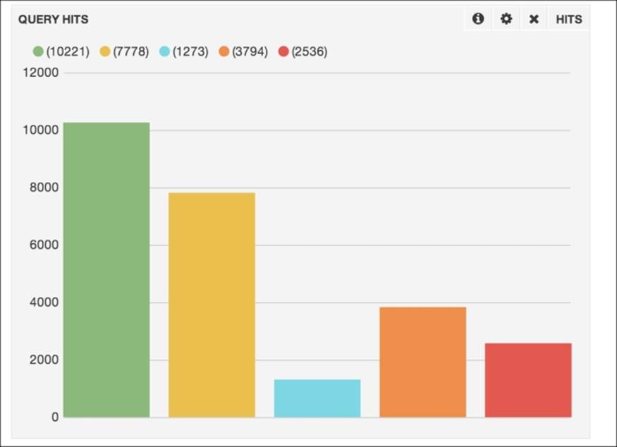
Terms aggregation are very useful for representing an overview of values used for further filtering. In a graph, they are often shown as a bar chart, as follows:
There's more…
Sometimes, we need to have much more control over terms aggregation; this can be achieved by adding an ElasticSearch script in the script field.
With scripting, it is possible to modify the term used for the aggregation to generate a new value that can be used. A simple example, in which we append the 123 value to all the terms, is as follows:
{
"query" : {
"match_all" : { }
},
"aggs" : {
"tag" : {
"terms" : {
"field" : "tag",
"script" : "_value + '123'"
}
}
}
}
Scripting can also be used to control the inclusion/exclusion of some terms. In this case, the returned value from the script must be a Boolean (true/false). If we want an aggregation with terms that start with the a character, we can use a similar aggregation:
{
"query" : {
"match_all" : { }
},
"aggs" : {
"tag" : {
"terms" : {
"field" : "tag",
"script" : "_value.startsWith('a')"
}
}
}
}
In the previous terms aggregation examples, we provided the field or fields parameter to select the field that is to be used to compute the aggregation. It's also possible to pass a script parameter that replaces field and fields in order to define the field to be used to extract the data. The script can fetch from the doc variable in the given context.
In the case of doc, the earlier example can be rewritten as:
… "tag": {
"terms": {
"script": "doc['tag'].value",
"size": 10
}
}
…
See also
· Chapter 7, Scripting, to know more about scripting
Executing the range aggregation
The previous recipe describes an aggregation type that can be very useful if a bucket must be computed on terms or on a limited number of items. Otherwise, it's often required to return the buckets that are aggregated in ranges—the range aggregation answers this requirement. The commons scenarios in which this aggregation can be used are:
· Price ranges (used in shops)
· Size ranges
· Alphabetical ranges
Getting ready
You need a working ElasticSearch cluster and an index populated with the script (chapter_06/executing_range_aggregations.sh) available at https://github.com/aparo/elasticsearch-cookbook-second-edition.
How to do it...
To execute range aggregations, we will perform the steps given as follows:
1. We want to provide three types of aggregation ranges, as follows:
· Price aggregation: This method aggregates the price of the items in a range
· Age aggregation: This method aggregates the age contained in a document in four ranges of 25 years
· Date aggregation: This method aggregates the ranges of 6 months of the previous year and all months this year
2. To obtain this result, we need to execute a query, as follows:
3. curl -XGET 'http://127.0.0.1:9200/test-index/test-type/_search?pretty=true&size=0' -d ' {
4. "query": {
5. "match_all": {}
6. },
7. "aggs": {
8. "prices": {
9. "range": {
10. "field": "price",
11. "ranges": [
12. {"to": 10},
13. {"from": 10,"to": 20},
14. {"from": 20,"to": 100},
15. {"from": 100}
16. ]
17. }
18. },
19. "ages": {
20. "range": {
21. "field": "age",
22. "ranges": [
23. {"to": 25},
24. {"from": 25,"to": 50},
25. {"from": 50,"to": 75},
26. {"from": 75}
27. ]
28. }
29. },
30. "range": {
31. "range": {
32. "field": "date",
33. "ranges": [
34. {"from": "2012-01-01","to": "2012-07-01"},
35. {"from": "2012-07-01","to": "2012-12-31"},
36. {"from": "2013-01-01","to": "2013-12-31"}
37. ]
38. }
39. }
40. }
41.}'
42. The results will be something like the following:
43.{
44. "took" : 7,
45. "timed_out" : false,
46. "_shards" : {…truncated…},
47. "hits" : {…truncated…},
48. "aggregations" : {
49. "range" : {
50. "buckets" : [ {
51. "key" : "20120101-01-01T00:00:00.000Z-20120631-01-01T00:00:00.000Z",
52. "from" : 6.348668943168E17,
53. "from_as_string" : "20120101-01-01T00:00:00.000Z",
54. "to" : 6.34883619456E17,
55. "to_as_string" : "20120631-01-01T00:00:00.000Z",
56. "doc_count" : 0
57. }, …truncated… ]
58. },
59. "prices" : {
60. "buckets" : [ {
61. "key" : "*-10.0",
62. "to" : 10.0,
63. "to_as_string" : "10.0",
64. "doc_count" : 105
65. }, …truncated…]
66. },
67. "ages" : {
68. "buckets" : [ {
69. "key" : "*-25.0",
70. "to" : 25.0,
71. "to_as_string" : "25.0",
72. "doc_count" : 210
73. }, …truncated…]
74. }
75. }
}
Every aggregation result has the following fields:
· The to, to_string, from, and from_string fields that define the original range of the aggregation
· doc_count: This gives the number of results in this range
· key: This is a string representation of the range
How it works...
This kind of aggregation is generally executed on numerical data types (integer, float, long, and dates). It can be considered as a list of range filters executed on the result of the query.
Date/date-time values, when used in a filter/query, must be expressed in string format; the valid string formats are yyyy-MM-dd'T'HH:mm:ss and yyyy-MM-dd.
Each range is computed independently; thus, in their definition, they can overlap.
There's more…
There are two special range aggregations used to target date and IPv4 ranges.
They are similar to the range aggregation, but they provide special functionalities to control date and IP address ranges.
The date range aggregation (date_range) defines the from and to fields in Date Math expressions. For example, to execute an aggregation of hits of before and after a 6-month period, the aggregation will be as follows:
{
"aggs": {
"range": {
"date_range": {
"field": "date",
"format": "MM-yyyy",
"ranges": [
{ "to": "now-6M/M" },
{ "from": "now-6M/M" }
]
}
}
}
}
In the preceding example, the buckets will be formatted in the form of month-year (MM-YYYY) in two ranges. The now parameter defines the actual date-time, -6M means minus 6 months, and /M is a shortcut for division using the month value. (A complete reference on Date Math expressions and code is available at http://www.elasticsearch.org/guide/en/elasticsearch/reference/current/search-aggregations-bucket-daterange-aggregation.html.)
The IPv4 range aggregation (ip_range) defines the ranges in the following formats:
· The IP range form:
· {
· "aggs" : {
· "ip_ranges" : {
· "ip_range" : {
· "field" : "ip",
· "ranges" : [
· { "to" : "192.168.1.1" },
· { "from" : "192.168.2.255" }
· ]
· }
· }
· }
}
· CIDR masks:
· {
· "aggs" : {
· "ip_ranges" : {
· "ip_range" : {
· "field" : "ip",
· "ranges" : [
· { "mask" : "192.168.1.0/25" },
· { "mask" : "192.168.1.127/25" }
· ]
· }
· }
· }
}
See also
· The Using a range query/filter recipe in Chapter 5, Search, Queries, and Filters
Executing the histogram aggregation
ElasticSearch numerical values can be used to process histogram data. The histogram representation is a very powerful way to show data to end users.
Getting ready
You need a working ElasticSearch cluster and an index populated with the script (chapter_06/executing_histogram_aggregations.sh) available at https://github.com/aparo/elasticsearch-cookbook-second-edition.
How to do it...
Using the items populated with the script, we want to calculate aggregations on:
· Age with an interval of 5 years
· Price with an interval of 10$
· Date with an interval of 6 months
To execute histogram aggregations, we will perform the steps given as follows:
1. The query will be as follows:
2. curl -XGET 'http://127.0.0.1:9200/test-index/test-type/_search?pretty=true&size=0' -d '{
3. "query": {
4. "match_all": {}
5. },
6. "aggregations": {
7. "age" : {
8. "histogram" : {
9. "field" : "age",
10. "interval" : 5
11. }
12. },
13. "price" : {
14. "histogram" : {
15. "field" : "price",
16. "interval" : 10.0
17. }
18. }
19. }
}'
20. The result (stripped) will be:
21.{
22. "took" : 23,
23. "timed_out" : false,
24. "_shards" : {…truncated…},
25. "hits" : {…truncated…},
26. "aggregations" : {
27. "price" : {
28. "buckets" : [ {
29. "key_as_string" : "0",
30. "key" : 0,
31. "doc_count" : 105
32. }, {
33. "key_as_string" : "10",
34. "key" : 10,
35. "doc_count" : 107
36. …truncated… } ]
37. },
38. "age" : {
39. "buckets" : [ {
40. "key_as_string" : "0",
41. "key" : 0,
42. "doc_count" : 34
43. }, {
44. "key_as_string" : "5",
45. "key" : 5,
46. "doc_count" : 41
47. }, {…truncated… } ]
48. }
49. }
}
The aggregation result is composed of buckets: a list of aggregation results. These results are composed of the following:
· key: This is the value that is always on the x axis on the histogram graph
· key_as_string: This is a string representation of the key value
· doc_count: This denotes the document bucket size
How it works...
This kind of aggregation is calculated in a distributed manner, in each shard with search results, and then the aggregation results are aggregated in the search node server (arbiter), which is then returned to the user.
The histogram aggregation works only on numerical fields (Boolean, Integer, long Integer, float) and date/date-time fields (that are internally represented as long). To control histogram generation on a defined field, the interval parameter is required, which is used to generate an interval to aggregate the hits.
For numerical fields, this value is a number (in the preceding example, we have done numerical calculation on age and price).
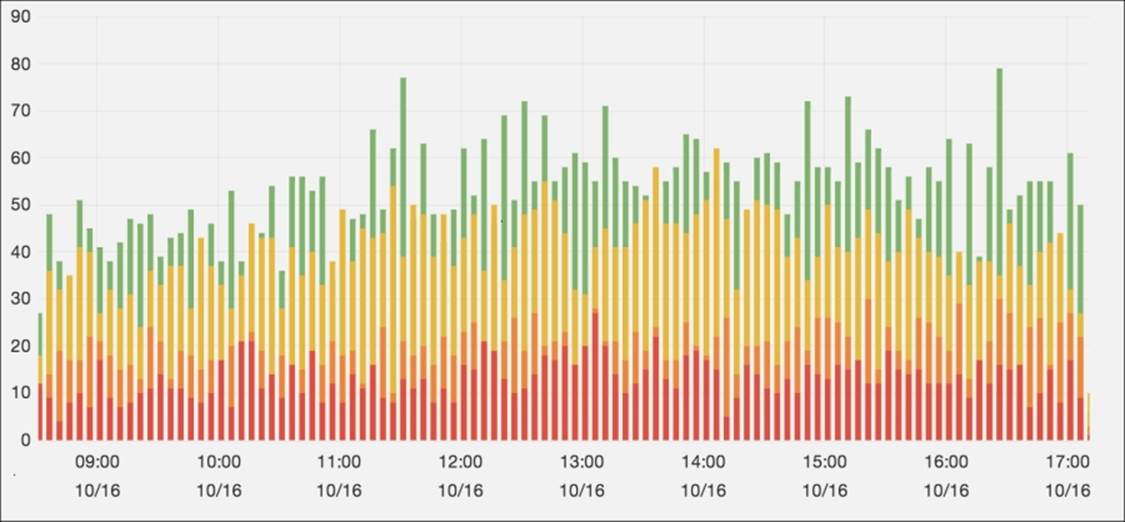
The general representation of a histogram can be a bar chart, similar to the following:
There's more…
Histogram aggregations can be also improved using ElasticSearch scripting functionalities. It is possible to script using _value if a field is stored or via the doc variable.
An example of a scripted aggregation histogram using _value is as follows:
curl -XGET 'http://127.0.0.1:9200/test-index/test-type/_search?&pretty=true&size=0' -d '{
"query": {
"match_all": {}
},
"aggs": {
"age" : {
"histogram" : {
"field" : "age",
"script": "_value*3",
"interval" : 5
}
}
}
}'
An example of a scripted aggregation histogram using _doc is as follows:
curl -XGET 'http://127.0.0.1:9200/test-index/test-type/_search?&pretty=true&size=0' -d '{
"query": {
"match_all": {}
},
"aggs": {
"age" : {
"histogram" : {
"script": "doc['age'].value",
"interval" : 5
}
}
}
}'
See also
· The Executing the date histogram aggregation recipe
Executing the date histogram aggregation
The previous recipe works mainly on numeric fields; ElasticSearch provides a custom date histogram aggregation to operate on date/date-time values. This aggregation is required because date values need more customization to solve problems such as time zone conversion and special time intervals.
Getting ready
You need a working ElasticSearch cluster and an index populated with the script (chapter_06/executing_date_histogram_aggregations.sh) available at https://github.com/aparo/elasticsearch-cookbook-second-edition.
How to do it...
We need two different date/time aggregations that are:
· An annual aggregation
· A quarter aggregation, but with time zone +1:00
To execute date histogram aggregations, we will perform the steps given as follows:
1. The query will be as follows:
2. curl -XGET 'http://127.0.0.1:9200/test-index/test-type/_search? pretty=true' -d '
3. {
4. "query": {
5. "match_all": {}
6. },
7. "aggs": {
8. "date_year": {
9. "date_histogram": {
10. "field": "date",
11. "interval": "year"
12. }
13. },
14. "date_quarter": {
15. "date_histogram": {
16. "field": "date",
17. "interval": "quarter" ,
18. "time_zone": "+01:00"
19. }
20. }
21. }
}'
22. The corresponding results are as follows:
23.{
24. "took" : 29,
25. "timed_out" : false,
26. "_shards" : {…truncated…},
27. "hits" : {…truncated…},
28. "aggregations" : {
29. "date_year" : {
30. "buckets" : [ {
31. "key_as_string" : "2010-01-01T00:00:00.000Z",
32. "key" : 1262304000000,
33. "doc_count" : 40
34. }, {
35. "key_as_string" : "2011-01-01T00:00:00.000Z",
36. "key" : 1293840000000,
37. "doc_count" : 182
38. }, …truncated…]
39. },
40. "date_quarter" : {
41. "buckets" : [ {
42. "key_as_string" : "2010-10-01T00:00:00.000Z",
43. "key" : 1285891200000,
44. "doc_count" : 40
45. }, {
46. "key_as_string" : "2011-01-01T00:00:00.000Z",
47. "key" : 1293840000000,
48. "doc_count" : 42
49. }, …truncated…]
50. }
51. }
}
The aggregation result is composed of buckets: a list of aggregation results. These results are composed of the following:
· key: This is the value that is always on the x axis on the histogram graph
· key_as_string: This is a string representation of the key value
· doc_count: This denotes the document bucket size
How it works...
The main difference in the preceding histogram recipe is that the interval is not numerical, but generally date intervals are defined time constants. The interval parameter allows us to use several values such as:
· Year
· Quarter
· Month
· Week
· Day
· Hour
· Minute
When working with date values, it's important to use the correct time zones to prevent query errors. By default, ElasticSearch uses the UTC milliseconds, from epoch, to store date-time values. To better handle the correct timestamp, there are some parameters that can be used such as:
· time_zone (or pre_zone, in which case it's is optional): This parameter allows defining a time zone offset to be used in value calculation. This value is used to preprocess the date-time value for the aggregation. The value can be expressed in numeric form (such as -3) if specifying hours or minutes, then it must be defined in the time zone. A string representation can be used (such as +07:30).
· post_zone (optional): This parameter takes the result and applies the time zone offset to that result.
· pre_zone_adjust_large_interval (by default, this is false and is optional): This parameter applies the hour interval also for day or above intervals.
See also
· Visit the official ElasticSearch documentation on date histogram aggregation at www.elasticsearch.org/guide/en/elasticsearch/reference/current/search-aggregations-bucket-datehistogram-aggregation.html for more details on managing time zone issues
Executing the filter aggregation
Sometimes, we need to reduce the number of hits in our aggregation to satisfy a particular filter. To obtain this result, the filter aggregation is used.
Getting ready
You need a working ElasticSearch cluster and an index populated with the script (chapter_06/test_filter_aggregation.sh) available at https://github.com/aparo/elasticsearch-cookbook-second-edition.
How to do it...
We need to compute two different filter aggregations that are:
· The count of documents that have ullam as tag
· The count of documents that have age equal to 37
To execute filter aggregations, we will perform the steps given as follows:
1. The query to execute these aggregations is as follows:
2. curl -XGET 'http://127.0.0.1:9200/test-index/test-type/_search?size=0&pretty=true' -d '
3. {
4. "query": {
5. "match_all": {}
6. },
7. "aggregations": {
8. "ullam_docs": {
9. "filter" : {
10. "term" : { "tag" : "ullam" }
11. }
12. },
13. "age37_docs": {
14. "filter" : {
15. "term" : { "age" : 37 }
16. }
17. }
18. }
19.}'
In this case, we have used simple filters, but they can be more complex if needed.
20. The results of the preceding query with aggregations will be as follows:
21.{
22. "took" : 5,
23. "timed_out" : false,
24. "_shards" : {
25. "total" : 5,
26. "successful" : 5,
27. "failed" : 0
28. },
29. "hits" : {
30. "total" : 1000,
31. "max_score" : 0.0,
32. "hits" : [ ]
33. },
34. "aggregations" : {
35. "age37_docs" : {
36. "doc_count" : 6
37. },
38. "ullam_docs" : {
39. "doc_count" : 17
40. }
41. }
}
How it works...
Filter aggregation is very simple; it executes a count on a filter in a matched element. You can consider this aggregation as a count query on the results. As we can see from the preceding result, the aggregation contains one value doc_count, which is the count result.
It can be seen as a very simple aggregation; generally, users tend not to use it as they prefer statistical aggregations, which also provide a count; alternatively, in the worst cases, they execute another search that generates more server workload.
The big advantage of this kind of aggregation is that the count, whenever possible, is executed via a filter, which is way faster than iterating all the results.
Another important advantage is that the filter can be composed of every possible valid Query DSL element.
There's more…
It's often required to have a document count that doesn't match a filter or generally doesn't have a particular field (or is null). For this kind of scenario, there is a special aggregation type: missing.
For example, to count the number of documents missing the code field, the query will be as follows:
curl -XGET 'http://127.0.0.1:9200/test-index/test-type/_search?size=0&pretty' -d '
{
"query": {
"match_all": {}
},
"aggs": {
"missing_code": {
"missing" : {
"field" : "code"
}
}
}
}'
The result will be as follows:
{
… truncated …
"aggregations" : {
"missin_code" : {
"doc_count" : 1000
}
}
}
See also
· The Counting matched results recipe in Chapter 5, Search, Queries, and Filters
· The Executing a scan query recipe in Chapter 5, Search, Queries, and Filters
Executing the global aggregation
Aggregations are generally executed on query search results, ElasticSearch provides a special aggregation—global—that is executed globally on all the documents without being influenced by the query.
Getting ready
You need a working ElasticSearch cluster and an index populated with the script (executing_global_aggregations.sh) available at https://github.com/aparo/elasticsearch-cookbook-second-edition.
How to do it...
To execute global aggregations, we will perform the steps given as follows:
1. If we want to compare a global average with a query one, the call will be something like this:
2. curl -XGET 'http://127.0.0.1:9200/test-index/test-type/_search?size=0&pretty=true' -d '
3. {
4. "query": {
5. "term" : { "tag" : "ullam" }
6. },
7. "aggregations": {
8. "query_age_avg": {
9. "avg" : {
10. "field" : "age"
11. }
12. },
13. "all_persons":{
14. "global": {},
15. "aggs":{
16. "age_global_avg": {
17. "avg" : {
18. "field" : "age"
19. }
20. }
21. }
22. }
23. }
24.}'
25. The result will be as follows:
26.{
27. "took" : 133,
28. "timed_out" : false,
29. "_shards" : {…truncated…},
30. "hits" : {
31. "total" : 17,
32. "max_score" : 0.0,
33. "hits" : [ ]
34. },
35. "aggregations" : {
36. "all_persons" : {
37. "doc_count" : 1000,
38. "age_global_avg" : {
39. "value" : 53.243
40. }
41. },
42. "query_age_avg" : {
43. "value" : 53.470588235294116
44. }
45. }
}
In the example, the query_age_avg function is computed on the query and the age_global_avg function on all the documents.
How it works...
This kind of aggregation is mainly used as top aggregation—that is, as a start point for other subaggregations. The body of the global aggregations is empty; it doesn't have any optional parameters. The most frequently used cases are comparative aggregations executed on filters with those without aggregation, as in the preceding example.
Executing the geo distance aggregation
Among the other standard types that we have seen in previous aggregations, ElasticSearch allows executing aggregations against a geo point: geo distance aggregations. This is an evolution of the previously discussed range aggregations built to work on geo locations.
Getting ready
You need a working ElasticSearch cluster and an index populated with the script (executing_geo_distance_aggregations.sh) available at https://github.com/aparo/elasticsearch-cookbook-second-edition.
How to do it...
Using the position field available in documents, we will aggregate the other documents in four ranges:
· Fewer than 10 kilometers
· From 10 to 20 kilometers
· From 20 to 50 kilometers
· From 50 to 100 kilometers
· Above 100 kilometers
To execute geo distance aggregations, we will perform the steps given as follows:
1. To achieve these goals, we will create a geo distance aggregation with a code similar to this one:
2. curl -XGET 'http://127.0.0.1:9200/test-index/test-type/_search?pretty=true&size=0' -d ' {
3. "query" : {
4. "match_all" : {}
5. },
6. "aggs" : {
7. "position" : {
8. "geo_distance" : {
9. "field":"position",
10. "origin" : {
11. "lat": 83.76,
12. "lon": -81.20
13. },
14. "ranges" : [
15. { "to" : 10 },
16. { "from" : 10, "to" : 20 },
17. { "from" : 20, "to" : 50 },
18. { "from" : 50, "to" : 100 },
19. { "from" : 100 }
20. ]
21. }
22. }
23. }
24.}'
25. The result will be as follows:
26.{
27. "took" : 177,
28. "timed_out" : false,
29. "_shards" : {…truncated…},
30. "hits" : {…truncated…},
31. "aggregations" : {
32. "position" : {
33. "buckets" : [ {
34. "key" : "*-10.0",
35. "from" : 0.0,
36. "to" : 10.0,
37. "doc_count" : 0
38. }, {
39. "key" : "10.0-20.0",
40. "from" : 10.0,
41. "to" : 20.0,
42. "doc_count" : 0
43. }, {
44. "key" : "20.0-50.0",
45. "from" : 20.0,
46. "to" : 50.0,
47. "doc_count" : 0
48. }, {
49. "key" : "50.0-100.0",
50. "from" : 50.0,
51. "to" : 100.0,
52. "doc_count" : 0
53. }, {
54. "key" : "100.0-*",
55. "from" : 100.0,
56. "doc_count" : 1000
57. } ]
58. }
59. }
}
How it works...
The geo range aggregation is an extension of the range aggregations that work on geo localizations. It works only if a field is mapped as a geo_point. The field can contain a single or multivalue geo point.
This aggregation requires at least three parameters:
· field: This is the field of the geo point to work on
· origin: This is the geo point to be used to compute the distances
· ranges: This is a list of ranges to collect documents based on their distance from the target point
The geo point can be defined in one of these accepted formats:
· Latitude and longitude as properties, such as {"lat": 83.76, "lon": -81.20 }
· Longitude and latitude as an array, such as [-81.20, 83.76]
· Latitude and longitude as a string, such as "83.76, -81.20"
· Geohash, for example, fnyk80
The ranges are defined as a couple of from/to values. If one of them is missing, they are considered as unbound. The metric system used for the range is by default set to kilometers—but by using the property unit, it's possible to set it to:
· mi or miles
· in or inch
· yd or yard
· km or kilometers
· m or meters
· cm or centimeter
· mm or millimeters
It's also possible to set how the distance is computed with the distance_type parameter. Valid values for this parameter are:
· arc: This uses the Arc Length formula. It is the most precise. (See http://en.wikipedia.org/wiki/Arc_length for more details on the arc length algorithm.)
· sloppy_arc (default): It's a faster implementation of the Arc Length formula, but is less precise.
· plane: This uses the plane distance formula. It is the most fastest of all and CPU-intensive, but it too is less precise.
As for the range filter, the range values are treated independently, so overlapping ranges are allowed.
When the results are returned, this aggregation provides a lot of information in its fields:
· from/to: This defines the analyzed range
· Key: This defines the string representation of the range
· doc_count: This defines the number of documents in the bucket that match the range
See also
· The Executing the range aggregation recipe in this chapter
· The Mapping a geo point field recipe in Chapter 3, Managing Mapping
· The geohash grid aggregation at http://www.elasticsearch.org/guide/en/elasticsearch/reference/current/search-aggregations-bucket-geohashgrid-aggregation.html
Executing nested aggregation
Nested aggregations allow us to execute analysis on nested documents. When working with complex structures, nested objects are very common.
Getting ready
You need a working ElasticSearch cluster and an index populated with the script available at https://github.com/aparo/elasticsearch-cookbook-second-edition.
How to do it...
To execute nested aggregations, we will perform the steps given as follows:
1. We must index documents with a nested type, as discussed in the Managing nested objects recipe in Chapter 3, Managing Mapping:
2. {
3. "product" : {
4. "properties" : {
5. "resellers" : {
6. "type" : "nested"
7. "properties" : {
8. "username" : { "type" : "string", "index" : "not_analyzed" },
9. "price" : { "type" : "double" }
10. }
11. },
12. "tags" : { "type" : "string", "index":"not_analyzed"}
13. }
14. }
}
15. To return the minimum price the products can be purchased at, we create a nested aggregation with code similar to this one:
16.curl -XGET 'http://127.0.0.1:9200/test-index/product/_search?pretty=true&size=0' -d ' {
17. "query" : {
18. "match" : { "name" : "my product" }
19. },
20. "aggs" : {
21. "resellers" : {
22. "nested" : {
23. "path" : "resellers"
24. },
25. "aggs" : {
26. "min_price" : { "min" : { "field" : "resellers.price" } }
27. }
28. }
29. }
30.}'
31. The result will be as follows:
32.{
33. "took" : 7,
34. "timed_out" : false,
35. "_shards" : {…truncated…},
36. "hits" : {…truncated…},
37. "aggregations": {
38. "resellers": {
39. "min_price": {
40. "value" : 130
41. }
42. }
43. }
}
In this case, the resulting aggregation is a simple min metric that we have already seen in the second recipe of this chapter.
How it works...
The nested aggregation requires only the path data of the field, which is relative to the parent and contains the nested documents.
After having defined the nested aggregation, all the other kinds of aggregations can be used in the subaggregations.
There's more…
ElasticSearch provides a way to aggregate values from nested documents to their parent; this aggregation is called reverse_nested.
In the preceding example, we can aggregate the top tags for the reseller with a similar query:
curl -XGET 'http://127.0.0.1:9200/test-index/product/_search?pretty=true&size=0' -d ' {
"query" : {
"match" : { "name" : "my product" }
}
"aggs" : {
"resellers" : {
"nested" : {
"path" : "resellers"
},
"aggs" : {
"top_resellers" : {
"terms" : {
"field" : "resellers.username"
}
},
"aggs" : {
"resellers_to_product" : {
"reverse_nested" : {},
"aggs" : {
"top_tags_per_reseller" : {
"terms" : { "field" : "tags" }
}
}
}
}
}
}
}
}'
In this example, there are several steps:
1. We aggregate initially for nested resellers data.
2. Having activated the nested resellers documents, we are able to term-aggregate by its username field (resellers.username).
3. From the top resellers aggregation, we go back to aggregate on the parent via "reverse_nested".
4. Now, we can aggregate tags of the parent document.
The response of the query is similar to this one:
{
"took" : 93,
"timed_out" : false,
"_shards" : {…truncated…},
"hits" : {…truncated…},
"aggregations": {
"resellers": {
"top_usernames": {
"buckets" : [
{
"key" : "username_1",
"doc_count" : 17,
"resellers_to_product" : {
"top_tags_per_reseller" : {
"buckets" : [
{
"key" : "tag1",
"doc_count" : 9
},…
]
}
},…
}
]
}
}
}
}
Executing the top hit aggregation
The top hit aggregation is different from the other aggregation types. All the previous aggregations have metric (simple values) or bucket values; the top hit aggregation returns buckets of search hits.
Generally, the top hit aggregation is used as a subaggregation so that the top matching documents can be aggregated in buckets.
Getting ready
You need a working ElasticSearch cluster and an index populated with the script (chapter_06/executing_top_hit_aggregations.sh) available at https://github.com/aparo/elasticsearch-cookbook-second-edition.
How to do it...
To execute a top hit aggregation, we will perform the steps given as follows:
1. We want to aggregate the documents hits by tag (tags) and return only the name field of documents with a maximum age (top_tag_hits). We'll execute the search and aggregation with the following command:
2. curl -XGET 'http://127.0.0.1:9200/test-index/test-type/_search' -d '{
3. "query": {
4. "match_all": {}
5. },
6. "size": 0,
7. "aggs": {
8. "tags": {
9. "terms": {
10. "field": "tag",
11. "size": 2
12. },
13. "aggs": {
14. "top_tag_hits": {
15. "top_hits": {
16. "sort": [
17. {
18. "age": {
19. "order": "desc"
20. }
21. }
22. ],
23. "_source": {
24. "include": [
25. "name"
26. ]
27. },
28. "size": 1
29. }
30. }
31. }
32. }
33. }
34.}'
35. The result will be as follows:
36.{
37. "took" : 5,
38. "timed_out" : false,
39. "_shards" : …truncated…,
40. "hits" : …truncated…,
41. "aggregations" : {
42. "tags" : {
43. "buckets" : [ {
44. "key" : "laborum",
45. "doc_count" : 18,
46. "top_tag_hits" : {
47. "hits" : {
48. "total" : 18,
49. "max_score" : null,
50. "hits" : [ {
51. "_index" : "test-index",
52. "_type" : "test-type",
53. "_id" : "730",
54. "_score" : null,
55. "_source":{"name":"Gladiator"},
56. "sort" : [ 90 ]
57. } ]
58. }
59. }
60. }, {
61. "key" : "sit",
62. "doc_count" : 10,
63. "top_tag_hits" : {
64. "hits" : {
65. "total" : 10,
66. "max_score" : null,
67. "hits" : [ {
68. "_index" : "test-index",
69. "_type" : "test-type",
70. "_id" : "732",
71. "_score" : null,
72. "_source":{"name":"Masked Marvel"},
73. "sort" : [ 96 ]
74. } ]
75. }
76. }
77. } ]
78. }
79. }
}
How it works...
The top hit aggregation allows collecting buckets of hits from another aggregation. It provides optional parameters to control the result's slicing. These are as follows:
· from (by default 0): This is the starting position of the hits in the bucket.
· size (by default, set to the parent bucket size): This is the hit bucket size.
· sort (by default score): This allows us to sort for different values. Its definition is similar to the search sort in Chapter 5, Search, Queries, and Filters.
To control the returned hits, it is possible to use the same parameters as used for a search:
· _source: This allows us to control the returned source. It can be disabled (false), partially returned (obj.*) , or can have multiple exclude/include rules. In the earlier example, we have returned only the name field:
· "_source": {
· "include": [
· "name"
· ]
},
· highlighting: This allows us to define fields and settings to be used to calculate a query abstract.
· fielddata_fields: This allows us to return field data representation of your field.
· explain: This returns information on how the score is calculated for a particular document.
· version (by default false): This adds the version of a document in the results.
Tip
Top hit aggregation can be used to implement a field collapsing feature; this is done by using first a terms aggregation on the field that we want to collapse and then collecting the documents with a top hit aggregation.
See Also
· The Executing a search recipe in Chapter 5, Search, Queries, and Filters
· The Executing the terms aggregation recipe in this chapter
All materials on the site are licensed Creative Commons Attribution-Sharealike 3.0 Unported CC BY-SA 3.0 & GNU Free Documentation License (GFDL)
If you are the copyright holder of any material contained on our site and intend to remove it, please contact our site administrator for approval.
© 2016-2026 All site design rights belong to S.Y.A.