Mastering Elasticsearch, Second Edition (2015)
Chapter 3. Not Only Full Text Search
In the previous chapter, we extensively talked about querying in Elasticsearch. We started by looking at how default Apache Lucene scoring works, through how filtering works, and we've finished with looking at which query to use in a particular situation. In this chapter, we will continue with discussions regarding some of the Elasticsearch functionalities connected to both querying and data analysis. By the end of this chapter, we will have covered the following areas:
· What query rescoring is and how you can use it to optimize your queries and recalculate the score for some documents
· Controlling multimatch queries
· Analyzing your data to get significant terms from it
· Grouping your documents in buckets using Elasticsearch
· Differences in relationship handling when using object, nested documents, and parent–child functionality
· Extended information regarding Elasticsearch scripting such as Groovy usage and Lucene expressions
Query rescoring
One of the great features provided by Elasticsearch is the ability to change the ordering of documents after they were returned by a query. Actually, Elasticsearch does a simple trick—it recalculates the score of top matching documents, so only part of the document in the response is reordered. The reasons why we want to do that can vary. One of the reasons may be performance—for example, calculating target ordering is very costly because scripts are used and we would like to do this on the subset of documents returned by the original query. You can imagine that rescore gives us many great opportunities for business use cases. Now, let's look at this functionality and how we can benefit from using it.
What is query rescoring?
Rescore in Elasticsearch is the process of recalculating the score for a defined number of documents returned by the query. This means that Elasticsearch first takes N documents for a given query (or the post_filter phase) and calculates their score using a provided rescore definition. For example, if we would take a term query and ask for all the documents that are available, we can use rescore to recalculate the score for 100 documents only, not for all documents returned by the query. Please note that the rescore phase will not be executed when using search_type of scan or count. This means that rescore won't be taken into consideration in such cases.
An example query
Let's start with a simple query that looks as follows:
{
"fields" : ["title", "available"],
"query" : {
"match_all" : {}
}
}
It returns all the documents from the index the query is run against. Every document returned by the query will have the score equal to 1.0 because of the match_all query. This is enough to show how rescore affects our result set.
Structure of the rescore query
Let's now modify our query so that it uses the rescore functionality. Basically, let's assume that we want the score of the document to be equal to the value of the year field. The query that does that would look as follows:
{
"fields": ["title", "available"],
"query": {
"match_all": {}
},
"rescore": {
"query": {
"rescore_query": {
"function_score": {
"query": {
"match_all": {}
},
"script_score": {
"script": "doc['year'].value"
}
}
}
}
}
}
Note
Please note that you need to specify the lang property with the groovy value in the preceding query if you are using Elasticsearch 1.4 or older. What's more, the preceding example uses dynamic scripting which was enabled in Elasticsearch until versions 1.3.8 and 1.4.3 for groovy and till 1.2 for MVEL. If you would like to use dynamic scripting with groovy you should add script.groovy.sandbox.enabled property and set it to true in your elasticsearch.yml file. However, please remember that this is a security risk.
Let's now look at the preceding query in more detail. The first thing you may have noticed is the rescore object. The mentioned object holds the query that will affect the scoring of the documents returned by the query. In our case, the logic is very simple—just assign the value of the year field as the score of the document. Please also note, that when using curl you need to escape the script value, so the doc['year'].value would look like doc[\"year\"].value
Note
In the preceding example, in the rescore object, you can see a query object. When this book was written, a query object was the only option, but in future versions, we may expect other ways to affect the resulting score.
If we save this query in the query.json file and send it using the following command:
curl localhost:9200/library/book/_search?pretty -d @query.json
The document that Elasticsearch should return should be as follows (please note that we've omitted the structure of the response so that it is as simple as it can be):
{
"took" : 1,
"timed_out" : false,
"_shards" : {
"total" : 5,
"successful" : 5,
"failed" : 0
},
"hits" : {
"total" : 6,
"max_score" : 1962.0,
"hits" : [ {
"_index" : "library",
"_type" : "book",
"_id" : "2",
"_score" : 1962.0,
"fields" : {
"title" : [ "Catch-22" ],
"available" : [ false ]
}
}, {
"_index" : "library",
"_type" : "book",
"_id" : "3",
"_score" : 1937.0,
"fields" : {
"title" : [ "The Complete Sherlock Holmes" ],
"available" : [ false ]
}
}, {
"_index" : "library",
"_type" : "book",
"_id" : "1",
"_score" : 1930.0,
"fields" : {
"title" : [ "All Quiet on the Western Front" ],
"available" : [ true ]
}
}, {
"_index" : "library",
"_type" : "book",
"_id" : "6",
"_score" : 1905.0,
"fields" : {
"title" : [ "The Peasants" ],
"available" : [ true ]
}
}, {
"_index" : "library",
"_type" : "book",
"_id" : "4",
"_score" : 1887.0,
"fields" : {
"title" : [ "Crime and Punishment" ],
"available" : [ true ]
}
}, {
"_index" : "library",
"_type" : "book",
"_id" : "5",
"_score" : 1775.0,
"fields" : {
"title" : [ "The Sorrows of Young Werther" ],
"available" : [ true ]
}
} ]
}
}
As we can see, Elasticsearch found all the documents from the original query. Now look at the score of the documents. Elasticsearch took the first N documents and applied the second query to them. In the result, the score of those documents is the sum of the score from the first and second queries.
As you know, scripts execution can be demanding when it comes to performance. That's why we've used it in the rescore phase of the query. If our initial match_all query would return thousands of results, calculating script-based scoring for all those can affect query performance. Rescore gave us the possibility to only calculate such scoring on the top N documents and thus reduce the performance impact.
Note
In our example, we have only seen a single rescore definition. Since Elasticsearch 1.1.0, there is a possibility of defining multiple rescore queries for a single result set. Thanks to this, you can build multilevel queries when the top N documents are reordered and this result is an input for the next reordering.
Now let's see how to tune rescore functionality behavior and what parameters are available.
Rescore parameters
In the query under the rescore object, we are allowed to use the following parameters:
· window_size (defaults to the sum of the from and size parameters): The number of documents used for rescoring on every shard
· query_weight (defaults to 1): The resulting score of the original query will be multiplied by this value before adding the score generated by rescore
· rescore_query_weight (defaults to 1): The resulting score of the rescore will be multiplied by this value before adding the score generated by the original query
To sum up, the target score for the document is equal to:
original_query_score * query_weight + rescore_query_score * rescore_query_weight
Choosing the scoring mode
By default, the score from the original query part and the score from the rescored part are added together. However, we can control that by specifying the score_mode parameter. The available values for it are as follows:
· total: Score values are added together (the default behavior)
· multiply: Values are multiplied by each other
· avg: The result score is an average of enclosed scores
· max: The result is equals of greater score value
· min: The result is equals of lower score value
To sum up
Sometimes, we want to show results, where the ordering of the first documents on the page is affected by some additional rules. Unfortunately, this cannot be achieved by the rescore functionality. The first idea points to the window_size parameter, but this parameter, in fact, is not connected with the first documents on the result list but with the number of results returned on every shard. In addition, the window_size value cannot be less than page size (Elasticsearch will set the window_size value to the value of the size property, when window_size is lower than size). Also, one very important thing, rescoring cannot be combined with sorting because sorting is done before the changes to the documents, score are done by rescoring, and thus sorting won't take the newly calculated score into consideration.
Controlling multimatching
Until Elasticsearch 1.1, we had limited control over the multi_match query. Of course, we had the possibility to specify the fields we want our query to be run against; we could use disjunction max queries (by setting the use_dis_max property to true). Finally, we could inform Elasticsearch about the importance of each field by using boosting. Our example query run against multiple fields could look as follows:
curl -XGET 'localhost:9200/library/_search?pretty' -d '{
"query" : {
"multi_match" : {
"query" : "complete conan doyle",
"fields" : [ "title^20", "author^10", "characters" ]
}
}
}'
A simple query that will match documents having given tokens in any of the mentioned fields. In addition to that required query, the title field is more important than the author field, and finally the characters field.
Of course, we could also use the disjunction max query:
curl -XGET 'localhost:9200/library/_search?pretty' -d '{
"query" : {
"multi_match" : {
"query" : "complete conan doyle",
"fields" : [ "title^20", "author^10", "characters" ],
"use_dis_max" : true
}
}
}'
But apart from the score calculation for the resulting documents, using disjunction max didn't change much.
Multimatch types
With the release of Elasticsearch 1.1, the use_dis_max property was deprecated and Elasticsearch developers introduced a new property—the type. This property allows control over how the multi_match query is internally executed. Let's now look at the possibilities of controlling how Elasticsearch runs queries against multiple fields.
Note
Please note that the tie_breaker property was not deprecated and we can still use it without worrying about future compatibility.
Best fields matching
To use the best fields type matching, one should set the type property of the multi_match query to the best_fields query. This type of multimatching will generate a match query for each field specified in the fields property and it is best used for searching for multiple words in the same, best matching field. For example, let's look at the following query:
curl -XGET 'localhost:9200/library/_search?pretty' -d '{
"query" : {
"multi_match" : {
"query" : "complete conan doyle",
"fields" : [ "title", "author", "characters" ],
"type" : "best_fields",
"tie_breaker" : 0.8
}
}
}'
The preceding query would be translated into a query similar to the following one:
curl -XGET 'localhost:9200/library/_search?pretty' -d '{
"query" : {
"dis_max" : {
"queries" : [
{
"match" : {
"title" : "complete conan doyle"
}
},
{
"match" : {
"author" : "complete conan doyle"
}
},
{
"match" : {
"characters" : "complete conan doyle"
}
}
],
"tie_breaker" : 0.8
}
}
}'
If you would look at the results for both of the preceding queries, you would notice the following:
{
"took" : 1,
"timed_out" : false,
"_shards" : {
"total" : 5,
"successful" : 5,
"failed" : 0
},
"hits" : {
"total" : 1,
"max_score" : 0.033352755,
"hits" : [ {
"_index" : "library",
"_type" : "book",
"_id" : "3",
"_score" : 0.033352755,
"_source":{ "title": "The Complete Sherlock Holmes","author": "Arthur Conan Doyle","year": 1936,"characters": ["Sherlock Holmes","Dr. Watson", "G. Lestrade"],"tags": [],"copies": 0, "available" : false, "section" : 12}
} ]
}
}
Both queries resulted in exactly the same results and the same scores calculated for the document. One thing to remember is how the score is calculated. If the tie_breaker value is present, the score for each document is the sum of the score for the best matching field and the score of the other matching fields multiplied by the tie_breaker value. If the tie_breaker value is not present, the document is assigned the score equal to the score of the best matching field.
There is one more question when it comes to the best_fields matching: what happens when we would like to use the AND operator or the minimum_should_match property? The answer is simple: the best_fields matching is translated into many match queries and both the operator property and the minimum_should_match property are applied to each of the generated match queries. Because of that, a query as follows wouldn't return any documents in our case:
curl -XGET 'localhost:9200/library/_search?pretty' -d '{
"query" : {
"multi_match" : {
"query" : "complete conan doyle",
"fields" : [ "title", "author", "characters" ],
"type" : "best_fields",
"operator" : "and"
}
}
}'
This is because the preceding query would be translated into:
curl -XGET 'localhost:9200/library/_search?pretty' -d '{
"query" : {
"dis_max" : {
"queries" : [
{
"match" : {
"title" : {
"query" : "complete conan doyle",
"operator" : "and"
}
}
},
{
"match" : {
"author" : {
"query" : "complete conan doyle",
"operator" : "and"
}
}
},
{
"match" : {
"characters" : {
"query" : "complete conan doyle",
"operator" : "and"
}
}
}
]
}
}
}'
And the preceding query looks as follows on the Lucene level:
(+title:complete +title:conan +title:doyle) | (+author:complete +author:conan +author:doyle) | (+characters:complete +characters:conan +characters:doyle)
We don't have any document in the index that has the complete, conan, and doyle terms in a single field. However, if we would like to match the terms in a different field, we can use the cross-field matching.
Cross fields matching
The cross_fields type matching is perfect when we want all the terms from the query to be found in the mentioned fields inside the same document. Let's recall our previous query, but this time instead of the best_fields matching, let's use the cross_fields matching type:
curl -XGET 'localhost:9200/library/_search?pretty' -d '{
"query" : {
"multi_match" : {
"query" : "complete conan doyle",
"fields" : [ "title", "author", "characters" ],
"type" : "cross_fields",
"operator" : "and"
}
}
}'
This time, the results returned by Elasticsearch were as follows:
{
"took" : 1,
"timed_out" : false,
"_shards" : {
"total" : 5,
"successful" : 5,
"failed" : 0
},
"hits" : {
"total" : 1,
"max_score" : 0.08154379,
"hits" : [ {
"_index" : "library",
"_type" : "book",
"_id" : "3",
"_score" : 0.08154379,
"_source":{ "title": "The Complete Sherlock Holmes","author": "Arthur Conan Doyle","year": 1936,"characters": ["Sherlock Holmes","Dr. Watson", "G. Lestrade"],"tags": [],"copies": 0, "available" : false, "section" : 12}
} ]
}
}
This is because our query was translated into the following Lucene query:
+(title:complete author:complete characters:complete) +(title:conan author:conan characters:conan) +(title:doyle author:doyle characters:doyle)
The results will only contain documents having all the terms in any of the mentioned fields. Of course, this is only the case when we use the AND Boolean operator. With the OR operator, we will get documents having at least a single match in any of the fields.
One more thing that is taken care of when using the cross_fields type is the problem of different term frequencies for each field. Elasticsearch handles that by blending the term frequencies for all the fields that are mentioned in a query. To put it simply, Elasticsearch gives almost the same weight to all the terms in the fields that are used in a query.
Most fields matching
Another type of multi_field configuration is the most_fields type. As the official documentation states, it was designed to help run queries against documents that contain the same text analyzed in different ways. One of the examples is having multiple languages in different fields. For example, if we would like to search for books that have die leiden terms in their title or original title, we could run the following query:
curl -XGET 'localhost:9200/library/_search?pretty' -d '{
"query" : {
"multi_match" : {
"query" : "Die Leiden",
"fields" : [ "title", "otitle" ],
"type" : "most_fields"
}
}
}'
Internally, the preceding request would be translated to the following query:
curl -XGET 'localhost:9200/library/_search?pretty' -d '{
"query" : {
"bool" : {
"should" : [
{
"match" : {
"title" : "die leiden"
}
},
{
"match" : {
"otitle" : "die leiden"
}
}
]
}
}
}'
The resulting documents are given a score equal to the sum of scores from each match query divided by the number of matching match clauses.
Phrase matching
The phrase matching is very similar to the best_fields matching we already discussed. However, instead of translating the query using match queries, it uses match_phrase queries. Let's take a look at the following query:
curl -XGET 'localhost:9200/library/_search?pretty' -d '{
"query" : {
"multi_match" : {
"query" : "sherlock holmes",
"fields" : [ "title", "author" ],
"type" : "phrase"
}
}
}'
Because we use the phrase matching, it would be translated into the following:
curl -XGET 'localhost:9200/library/_search?pretty' -d '{
"query" : {
"dis_max" : {
"queries" : [
{
"match_phrase" : {
"title" : "sherlock holmes"
}
},
{
"match_phrase" : {
"author" : "sherlock holmes"
}
}
]
}
}
}'
Phrase with prefixes matching
This is exactly the same as the phrase matching, but instead of using match_phrase query, the match_phrase_prefix query is used. Let's assume we run the following query:
curl -XGET 'localhost:9200/library/_search?pretty' -d '{
"query" : {
"multi_match" : {
"query" : "sherlock hol",
"fields" : [ "title", "author" ],
"type" : "phrase_prefix"
}
}
}'
What Elasticsearch would do internally is run a query similar to the following one:
curl -XGET 'localhost:9200/library/_search?pretty' -d '{
"query" : {
"dis_max" : {
"queries" : [
{
"match_phrase_prefix" : {
"title" : "sherlock hol"
}
},
{
"match_phrase_prefix" : {
"author" : "sherlock hol"
}
}
]
}
}
}'
As you can see, by using the type property of the multi_match query, you can achieve different results without the need of writing complicated queries. What's more, Elasticsearch will also take care of the scoring and problems related to it.
Significant terms aggregation
One of the aggregations introduced after the release of Elasticsearch 1.0 is the significant_terms aggregation that we can use starting from release 1.1. It allows us to get the terms that are relevant and probably the most significant for a given query. The good thing is that it doesn't only show the top terms from the results of the given query, but also shows the one that seems to be the most important one.
The use cases for this aggregation type can vary from finding the most troublesome server working in your application environment to suggesting nicknames from the text. Whenever Elasticsearch can see a significant change in the popularity of a term, such a term is a candidate for being significant.
Note
Please remember that the significant_terms aggregation is marked as experimental and can change or even be removed in the future versions of Elasticsearch.
An example
The best way to describe the significant_terms aggregation type will be through an example. Let's start with indexing 12 simple documents, which represent reviews of work done by interns (commands are also provided in a significant.sh script for easier execution on Linux-based systems):
curl -XPOST 'localhost:9200/interns/review/1' -d '{"intern" : "Richard", "grade" : "bad", "type" : "grade"}'
curl -XPOST 'localhost:9200/interns/review/2' -d '{"intern" : "Ralf", "grade" : "perfect", "type" : "grade"}'
curl -XPOST 'localhost:9200/interns/review/3' -d '{"intern" : "Richard", "grade" : "bad", "type" : "grade"}'
curl -XPOST 'localhost:9200/interns/review/4' -d '{"intern" : "Richard", "grade" : "bad", "type" : "review"}'
curl -XPOST 'localhost:9200/interns/review/5' -d '{"intern" : "Richard", "grade" : "good", "type" : "grade"}'
curl -XPOST 'localhost:9200/interns/review/6' -d '{"intern" : "Ralf", "grade" : "good", "type" : "grade"}'
curl -XPOST 'localhost:9200/interns/review/7' -d '{"intern" : "Ralf", "grade" : "perfect", "type" : "review"}'
curl -XPOST 'localhost:9200/interns/review/8' -d '{"intern" : "Richard", "grade" : "medium", "type" : "review"}'
curl -XPOST 'localhost:9200/interns/review/9' -d '{"intern" : "Monica", "grade" : "medium", "type" : "grade"}'
curl -XPOST 'localhost:9200/interns/review/10' -d '{"intern" : "Monica", "grade" : "medium", "type" : "grade"}'
curl -XPOST 'localhost:9200/interns/review/11' -d '{"intern" : "Ralf", "grade" : "good", "type" : "grade"}'
curl -XPOST 'localhost:9200/interns/review/12' -d '{"intern" : "Ralf", "grade" : "good", "type" : "grade"}'
Of course, to show the real power of the significant_terms aggregation, we should use a way larger dataset. However, for the purpose of this book, we will concentrate on this example, so it is easier to illustrate how this aggregation works.
Now let's try finding the most significant grade for Richard. To do that we will use the following query:
curl -XGET 'localhost:9200/interns/_search?pretty' -d '{
"query" : {
"match" : {
"intern" : "Richard"
}
},
"aggregations" : {
"description" : {
"significant_terms" : {
"field" : "grade"
}
}
}
}'
The result of the preceding query looks as follows:
{
"took" : 2,
"timed_out" : false,
"_shards" : {
"total" : 5,
"successful" : 5,
"failed" : 0
},
"hits" : {
"total" : 5,
"max_score" : 1.4054651,
"hits" : [ {
"_index" : "interns",
"_type" : "review",
"_id" : "4",
"_score" : 1.4054651,
"_source":{"intern" : "Richard", "grade" : "bad"}
}, {
"_index" : "interns",
"_type" : "review",
"_id" : "3",
"_score" : 1.0,
"_source":{"intern" : "Richard", "grade" : "bad"}
}, {
"_index" : "interns",
"_type" : "review",
"_id" : "8",
"_score" : 1.0,
"_source":{"intern" : "Richard", "grade" : "medium"}
}, {
"_index" : "interns",
"_type" : "review",
"_id" : "1",
"_score" : 1.0,
"_source":{"intern" : "Richard", "grade" : "bad"}
}, {
"_index" : "interns",
"_type" : "review",
"_id" : "5",
"_score" : 1.0,
"_source":{"intern" : "Richard", "grade" : "good"}
} ]
},
"aggregations" : {
"description" : {
"doc_count" : 5,
"buckets" : [ {
"key" : "bad",
"doc_count" : 3,
"score" : 0.84,
"bg_count" : 3
} ]
}
}
}
As you can see, for our query, Elasticsearch informed us that the most significant grade for Richard is bad. Maybe it wasn't the best internship for him, who knows.
Choosing significant terms
To calculate significant terms, Elasticsearch looks for data that reports significant changes in their popularity between two sets of data: the foreground set and the background set. The foreground set is the data returned by our query, while the background set is the data in our index (or indices, depending on how we run our queries). If a term exists in 10 documents out of 1 million indexed documents, but appears in five documents from 10 returned, such a term is definitely significant and worth concentrating on.
Let's get back to our preceding example now to analyze it a bit. Richard got three grades from the reviewers: bad three times, medium one time, and good one time. From those three, the bad value appears in three out of five documents matching the query. In general, the bad grade appears in three documents (the bg_count property) out of the 12 documents in the index (this is our background set). This gives us 25 percent of the indexed documents. On the other hand, the bad grade appears in three out of five documents matching the query (this is our foreground set), which gives us 60 percent of the documents. As you can see, the change in popularity is significant for the bad grade and that's why Elasticsearch have chosen it to be returned in the significant_terms aggregation results.
Multiple values analysis
Of course, the significant_terms aggregation can be nested and provide us with nice data analysis capabilities that connect two multiple sets of data. For example, let's try to find a significant grade for each of the interns that we have information about. To do that, we will nest the significant_terms aggregation inside the terms aggregation and the query that does that looks as follows:
curl -XGET 'localhost:9200/interns/_search?size=0&pretty' -d '{
"aggregations" : {
"grades" : {
"terms" : {
"field" : "intern"
},
"aggregations" : {
"significantGrades" : {
"significant_terms" : {
"field" : "grade"
}
}
}
}
}
}'
The results returned by Elasticsearch for that query are as follows:
{
"took" : 71,
"timed_out" : false,
"_shards" : {
"total" : 5,
"successful" : 5,
"failed" : 0
},
"hits" : {
"total" : 12,
"max_score" : 0.0,
"hits" : [ ]
},
"aggregations" : {
"grades" : {
"doc_count_error_upper_bound" : 0,
"sum_other_doc_count" : 0,
"buckets" : [ {
"key" : "ralf",
"doc_count" : 5,
"significantGrades" : {
"doc_count" : 5,
"buckets" : [ {
"key" : "good",
"doc_count" : 3,
"score" : 0.21000000000000002,
"bg_count" : 4
} ]
}
}, {
"key" : "richard",
"doc_count" : 5,
"significantGrades" : {
"doc_count" : 5,
"buckets" : [ {
"key" : "bad",
"doc_count" : 3,
"score" : 0.6,
"bg_count" : 3
} ]
}
}, {
"key" : "monica",
"doc_count" : 2,
"significantGrades" : {
"doc_count" : 2,
"buckets" : [ ]
}
} ]
}
}
}
As you can see, we got the results for interns Ralf (key property equals ralf) and Richard (key property equals richard). We didn't get information for Monica though. That's because there wasn't a significant change for the term in the grade field associated with themonica value in the intern field.
Significant terms aggregation and full text search fields
Of course, the significant_terms aggregation can also be used on full text search fields, practically useful for identifying text keywords. The thing is that, running this aggregation of analyzed fields may require a large amount of memory because Elasticsearch will attempt to load every term into the memory.
For example, we could run the significant_terms aggregation against the title field in our library index like the following:
curl -XGET 'localhost:9200/library/_search?size=0&pretty' -d '{
"query" : {
"term" : {
"available" : true
}
},
"aggregations" : {
"description" : {
"significant_terms" : {
"field" : "title"
}
}
}
}'
However, the results wouldn't bring us any useful insight in this case:
{
"took" : 2,
"timed_out" : false,
"_shards" : {
"total" : 5,
"successful" : 5,
"failed" : 0
},
"hits" : {
"total" : 4,
"max_score" : 0.0,
"hits" : [ ]
},
"aggregations" : {
"description" : {
"doc_count" : 4,
"buckets" : [ {
"key" : "the",
"doc_count" : 3,
"score" : 1.125,
"bg_count" : 3
} ]
}
}
}
The reason for this is that we don't have large enough data for the results to be meaningful. However, from a logical point of view, the the term is significant for the title field.
Additional configuration options
We could stop here and let you play with the significant_terms aggregation, but we will not. Instead, we will show you a few of the vast configuration options available for this aggregation type so that you can configure internal calculations and adjust it to your needs.
Controlling the number of returned buckets
Elasticsearch allows, how many buckets at maximum we want to have returned in the results. We can control it by using the size property. However, the final bucket list may contain more buckets than we set the size property to. This is the case when the number of unique terms is larger than the specified size property.
If you want to have even more control over the number of returned buckets, you can use the shard_size property. This property specifies how many candidates for significant terms will be returned by each shard. The thing to consider is that usually the low-frequency terms are the ones turning out to be the most interested ones, but Elasticsearch can't see that before merging the results on the aggregation node. Because of this, it is good to keep the shard_size property value higher than the value of the size property.
There is one more thing to remember: if you set the shard_size property lower than the size property, then Elasticsearch will replace the shard_size property with the value of the size property.
Note
Please note that starting from Elasticsearch 1.2.0, if the size or shard_size property is set to 0, Elasticsearch will change that and set it to Integer.MAX_VALUE.
Background set filtering
If you remember, we said that the background set of term frequencies used by the significant_terms aggregation is the whole index or indices. We can alter that behavior by using filter (using the background_filter property) to narrow down the background set. This is useful when we want to find significant terms in a given context.
For example, if we would like to narrow down the background set from our first example only to documents that are the real grades, not reviews, we would add the following term filter to our query:
curl -XGET 'localhost:9200/interns/_search?pretty&size=0' -d '{
"query" : {
"match" : {
"intern" : "Richard"
}
},
"aggregations" : {
"description" : {
"significant_terms" : {
"field" : "grade",
"background_filter" : {
"term" : {
"type" : "grade"
}
}
}
}
}
}'
If you would look more closely at the results, you would notice that Elasticsearch calculated the significant terms for a smaller number of documents:
{
"took" : 4,
"timed_out" : false,
"_shards" : {
"total" : 5,
"successful" : 5,
"failed" : 0
},
"hits" : {
"total" : 5,
"max_score" : 0.0,
"hits" : [ ]
},
"aggregations" : {
"description" : {
"doc_count" : 5,
"buckets" : [ {
"key" : "bad",
"doc_count" : 3,
"score" : 1.02,
"bg_count" : 2
} ]
}
}
}
Notice that bg_count is now 2 instead of 3 in the initial example. That's because there are only two documents having the bad value in the grade field and matching our filter specified in background_filter.
Minimum document count
A good thing about the significant_terms aggregation is that we can control the minimum number of documents a term needs to be present in to be included as a bucket. We do that by adding the min_doc_count property with the count of our choice.
For example, let's add this parameter to our query that resulted in significant grades for each of our interns. Let's lower the default value of 3 that the min_doc_count property is set to and let's set it to 2. Our modified query would look as follows:
curl -XGET 'localhost:9200/interns/_search?size=0&pretty' -d '{
"aggregations" : {
"grades" : {
"terms" : {
"field" : "intern"
},
"aggregations" : {
"significantGrades" : {
"significant_terms" : {
"field" : "grade",
"min_doc_count" : 2
}
}
}
}
}
}'
The results of the preceding query would be as follows:
{
"took" : 3,
"timed_out" : false,
"_shards" : {
"total" : 5,
"successful" : 5,
"failed" : 0
},
"hits" : {
"total" : 12,
"max_score" : 0.0,
"hits" : [ ]
},
"aggregations" : {
"grades" : {
"doc_count_error_upper_bound" : 0,
"sum_other_doc_count" : 0,
"buckets" : [ {
"key" : "ralf",
"doc_count" : 5,
"significantGrades" : {
"doc_count" : 5,
"buckets" : [ {
"key" : "perfect",
"doc_count" : 2,
"score" : 0.3200000000000001,
"bg_count" : 2
}, {
"key" : "good",
"doc_count" : 3,
"score" : 0.21000000000000002,
"bg_count" : 4
} ]
}
}, {
"key" : "richard",
"doc_count" : 5,
"significantGrades" : {
"doc_count" : 5,
"buckets" : [ {
"key" : "bad",
"doc_count" : 3,
"score" : 0.6,
"bg_count" : 3
} ]
}
}, {
"key" : "monica",
"doc_count" : 2,
"significantGrades" : {
"doc_count" : 2,
"buckets" : [ {
"key" : "medium",
"doc_count" : 2,
"score" : 1.0,
"bg_count" : 3
} ]
}
} ]
}
}
}
As you can see, the results differ from the original example—this is because the constraints on the significant terms have been lowered. Of course, that also means that our results may be worse now. Setting this parameter to 1 may result in typos and strange words being included in the results and is generally not advised.
There is one thing to remember when it comes to using the min_doc_count property. During the first phase of aggregation calculation, Elasticsearch will collect the highest scoring terms on each shard included in the process. However, because shard doesn't have the information about the global term frequencies, the decision about term being a candidate to a significant terms list is based on shard term frequencies. The min_doc_count property is applied during the final stage of the query, once all the results are merged from the shards. Because of this, it may happen that high-frequency terms are missing in the significant terms list and the list is populated by high-scoring terms instead. To avoid this, you can increase the shard_size property and the cost of memory consumption and higher network usage.
Execution hint
Elasticsearch allows us to specify execution mode, which should be used to calculate the significant_terms aggregation. Depending on the situation, we can either set the execution_hint property to map or to ordinal. The first execution type tells Elasticsearch to aggregate the data per bucket using the values themselves. The second value tells Elasticsearch to use ordinals of the values instead of the values themselves. In most situations, setting the execution_hint property to ordinal should result in slightly faster execution, but the data we are working on must expose the ordinals. However, if the fields you calculate the significant_terms aggregation on is high cardinality one (if it contains a high number of unique terms), then using map is, in most cases, a better choice.
Note
Please note that Elasticsearch will ignore the execution_hint property if it can't be applied.
More options
Because Elasticsearch is constantly being developed and changed, we decided not to include all the options that are possible to set. We also omitted the options that we think are very rarely used by the users so that we are able to write in further detail about more commonly used features. See the full list of options at http://www.elasticsearch.org/guide/en/elasticsearch/reference/current/search-aggregations-bucket-significantterms-aggregation.html.
There are limits
While we were working on this book, there were a few limitations when it comes to the significant_terms aggregation. Of course, those are no showstoppers that will force you to totally forget about that aggregation, but it is useful to know about them.
Memory consumption
Because the significant_terms aggregation works on indexed values, it needs to load all the unique terms into the memory to be able to do its job. Because of this, you have to be careful when using this aggregation on large indices and on fields that are analyzed. In addition to this, we can't lower the memory consumption by using doc values fields because the significant_terms aggregation doesn't support them.
Shouldn't be used as top-level aggregation
The significant_terms aggregation shouldn't be used as a top-level aggregation whenever you are using the match_all query, its equivalent returning all the documents or no query at all. In such cases, the foreground and background sets will be the same, and Elasticsearch won't be able to calculate the differences in frequencies. This means that no significant terms will be found.
Counts are approximated
Elasticsearch approximates the counts of how many documents contain a term based on the information returned for each shard. You have to be aware of that because this means that those counts can be miscalculated in certain situations (for example, count can be approximated too low when shards didn't include data for a given term in the top samples returned). As the documentation states, this was a design decision to allow faster execution at the cost of potentially small inaccuracies.
Floating point fields are not allowed
Fields that are floating point type-based ones are not allowed as the subject of calculation of the significant_terms aggregation. You can use the long or integer based fields though.
Documents grouping
One of the most desired functionalities in Elasticsearch was always a feature called document folding or document grouping. This functionality was the most +1 marked issue for Elasticsearch. It is not surprising at all. It is sometimes very convenient to show a list of documents grouped by a particular value, especially when the number of results is very big. In this case, instead of showing all the documents one by one, we would return only one (or a few) documents from every group. For example, in our library, we could prepare a query returning all the documents about wildlife sorted by publishing date, but limit the list to two books from every year. The other useful use case, where grouping can become very handy, is counting and showing distinct values in a field. An example of such behavior is returning only a single book that had many editions.
Top hits aggregation
The top_hits aggregation was introduced in Elasticsearch 1.3 along with the changes to scripting about which we will talk in the Scripting changes section later in this chapter. What is interesting is that we can force Elasticsearch to provide grouping functionality with this aggregation. In fact, it seems that a document folding is more or less a side effect and only one of the possible usage examples of the top_hits aggregation. In this section, we will only focus on how this particular aggregation works, and we assumed that you already know the basic rules that rule the world of the Elasticsearch aggregation framework.
Note
If you don't have any experience with this Elasticsearch functionality, please considering looking at Elasticsearch Server Second Edition published by Packt Publishing or reading the Elasticsearch documentation page available athttp://www.elasticsearch.org/guide/en/elasticsearch/reference/current/search-aggregations.html.
The idea behind the top_hits aggregation is simple. Every document that is assigned to a particular bucket can be also remembered. By default, only three documents per bucket are remembered. Let's see how it works using our example library index.
An example
To show you a potential use case that leverages the top_hits aggregation, we decided to use the following query:
curl -XGET "http://127.0.0.1:9200/library/_search?pretty" -d'
{
"size": 0,
"aggs": {
"when": {
"histogram": {
"field": "year",
"interval": 100
},
"aggs": {
"book": {
"top_hits": {
"_source": {
"include": [
"title",
"available"
]
},
"size": 1
}
}
}
}
}
}'
In the preceding example, we did the histogram aggregation on year ranges. Every bucket is created for every 100 years. The nested top_hits aggregations will remember a single document with the greatest score from each bucket (because of the size property set to 1). We added the include option only for simplicity of the results, so that we only return the title and available fields for every aggregated document. The response returned by Elasticsearch should be similar to the following one:
{
"took": 2,
"timed_out": false,
"_shards": {
"total": 5,
"successful": 5,
"failed": 0
},
"hits": {
"total": 4,
"max_score": 0,
"hits": []
},
"aggregations": {
"when": {
"buckets": [
{
"key_as_string": "1800",
"key": 1800,
"doc_count": 1,
"book": {
"hits": {
"total": 1,
"max_score": 1,
"hits": [
{
"_index": "library",
"_type": "book",
"_id": "4",
"_score": 1,
"_source": {
"title": "Crime and Punishment",
"available": true
}
}
]
}
}
},
{
"key_as_string": "1900",
"key": 1900,
"doc_count": 3,
"book": {
"hits": {
"total": 3,
"max_score": 1,
"hits": [
{
"_index": "library",
"_type": "book",
"_id": "3",
"_score": 1,
"_source": {
"title": "The Complete Sherlock Holmes",
"available": false
}
}
]
}
}
}
]
}
}
}
The interesting parts of the response are highlighted. We can see that because of the top_hits aggregation, we have the most scoring document (from each bucket) included in the response. In our particular case, the query was the match_all one and all the documents have the same score, so the top scoring document for every bucket is more or less random. Elasticsearch used the match_all query because we didn't specify any query at all—this is the default behavior. If we want to have a custom sorting, this is not a problem for Elasticsearch. For example, we can return the first book from a given century. What we just need to do is add a proper sorting option, just like in the following query:
curl -XGET 'http://127.0.0.1:9200/library/_search?pretty' -d '{
"size": 0,
"aggs": {
"when": {
"histogram": {
"field": "year",
"interval": 100
},
"aggs": {
"book": {
"top_hits": {
"sort": {
"year": "asc"
},
"_source": {
"include": [
"title",
"available"
]
},
"size": 1
}
}
}
}
}
}'
Please take a look at the highlighted fragment of the preceding query. We've added sorting to the top_hits aggregation, so the results are sorted on the basis of the year field. This means that the first document will be the one with the lowest value in that field and this is the document that is going to be returned for each bucket.
Additional parameters
However, sorting and field inclusion is not everything that we can we do inside the top_hits aggregation. Elasticsearch allows using several other functionalities related to documents retrieval. We don't want to discuss them all in detail because you should be familiar with most of them if you are familiar with the Elasticsearch aggregation module. However, for the purpose of this chapter, let's look at the following example:
curl -XGET 'http://127.0.0.1:9200/library/_search?pretty' -d '{
"query": {
"filtered": {
"query": {
"match": {
"_all": "quiet"
}
},
"filter": {
"term": {
"copies": 1,
"_name": "copies_filter"
}
}
}
},
"size": 0,
"aggs": {
"when": {
"histogram": {
"field": "year",
"interval": 100
},
"aggs": {
"book": {
"top_hits": {
"highlight": {
"fields": {
"title": {}
}
},
"explain": true,
"version": true,
"_source": {
"include": [
"title",
"available"
]
},
"fielddata_fields" : ["title"],
"script_fields": {
"century": {
"script": "(doc[\"year\"].value / 100).intValue()"
}
},
"size": 1
}
}
}
}
}
}'
As you can see, our query contains the following functionalities:
· Named filters and queries (in our example the filter is named copies_filter)
· Document version inclusion
· Document source filtering (choosing fields that should be returned)
· Using field-data fields and script fields
· Inclusion of explained information that tells us why a given document was matched and included
· Highlighting usage
Relations between documents
While Elasticsearch is gaining more and more attention, it is no longer used as a search engine only. It is seen as a data analysis solution and sometimes as a primary data store. Having a single data store that enables fast and efficient full text searching often seems like a good idea. We not only can store documents, but we can also search them and analyze their contents bringing meaning to the data. This is usually more than we could expect from traditional SQL databases. However, if you have any experience with SQL databases, when dealing with Elasticsearch, you soon realize the necessity of modeling relationships between documents. Unfortunately, it is not easy and many of the habits and good practices from relation databases won't work in the world of the inverted index that Elasticsearch uses. You should already be familiar with how Elasticsearch handles relationships because we already mentioned nested objects and parent–child functionality in our Elasticsearch Server Second Edition book, but let's go through available possibilities and look closer at the traps connected with them.
The object type
Elasticsearch tries to interfere as little as possible when modeling your data and turning it into an inverted index. Unlike the relation databases, Elasticsearch can index structured objects and it is natural to it. It means that if you have any JSON document, you can index it without problems and Elasticsearch adapts to it. Let's look at the following document:
{
"title": "Title",
"quantity": 100,
"edition": {
"isbn": "1234567890",
"circulation": 50000
}
}
As you can see, the preceding document has two simple properties and a nested object inside it (the edition one) with additional properties. The mapping for our example is simple and looks as follows (it is also stored in the relations.json file provided with the book):
{
"book" : {
"properties" : {
"title" : {"type": "string" },
"quantity" : {"type": "integer" },
"edition" : {
"type" : "object",
"properties" : {
"isbn" : {"type" : "string", "index" : "not_analyzed" },
"circulation" : {"type" : "integer" }
}
}
}
}
}
Unfortunately, everything will work only when the inner object is connected to its parent with a one-to-one relation. If you add the second object, for example, like the following:
{
"title": "Title",
"quantity": 100,
"edition": [
{
"isbn": "1234567890",
"circulation": 50000
},
{
"isbn": "9876543210",
"circulation": 2000
}
]
}
Elasticsearch will flatten it. To Elasticsearch, the preceding document will look more or less like the following one (of course, the _source field will still look like the preceding document):
{
"title": "Title",
"quantity": 100,
"edition": {
"isbn": [ "1234567890", "9876543210" ],
"circulation": [50000, 2000 ]
}
}
This is not exactly what we want, and such representation will cause problems when you search for books containing editions with given ISBN numbers and given circulation. Simply, cross-matches will happen—Elasticsearch will return books containing editions with given ISBNs and any circulation.
We can test this by indexing our document by using the following command:
curl -XPOST 'localhost:9200/object/doc/1' -d '{
"title": "Title",
"quantity": 100,
"edition": [
{
"isbn": "1234567890",
"circulation": 50000
},
{
"isbn": "9876543210",
"circulation": 2000
}
]
}'
Now, if we would run a simple query to return documents with the isbn field equal to 1234567890 and the circulation field equal to 2000, we shouldn't get any documents. Let's test that by running the following query:
curl -XGET 'localhost:9200/object/_search?pretty' -d '{
"fields" : [ "_id", "title" ],
"query" : {
"bool" : {
"must" : [
{
"term" : {
"isbn" : "1234567890"
}
},
{
"term" : {
"circulation" : 2000
}
}
]
}
}
}'
What we got as a result from Elasticsearch is as follows:
{
"took" : 5,
"timed_out" : false,
"_shards" : {
"total" : 5,
"successful" : 5,
"failed" : 0
},
"hits" : {
"total" : 1,
"max_score" : 1.0122644,
"hits" : [ {
"_index" : "object",
"_type" : "doc",
"_id" : "1",
"_score" : 1.0122644,
"fields" : {
"title" : [ "Title" ]
}
} ]
}
}
This cross-finding can be avoided by rearranging the mapping and document so that the source document looks like the following:
{
"title": "Title",
"quantity": 100,
"edition": {
"isbn": ["1234567890", "9876543210"],
"circulation_1234567890": 50000,
"circulation_9876543210": 2000
}
}
Now, you can use the preceding mentioned query, which use the relationships between fields by the cost of greater complexity of query building. The important problem is that the mappings would have to contain information about all the possible values of the fields—this is not something that we would like to go for when having more than a couple of possible values. From the other side, this still does not allow us to create more complicated queries such as all books with a circulation of more than 10 000 and ISBN number starting with 23. In such cases, a better solution would be to use nested objects.
To summarize, the object type could be handy only for the simplest cases when problems with cross-field searching does not exist—for example, when you don't want to search inside nested objects or you only need to search on one of the fields without matching on the others.
The nested documents
From the mapping point of view, the definition of a nested document differs only in the use of nested type instead of object (which Elasticsearch will use by default when guessing types). For example, let's modify our previous example so that it uses nested documents:
{
"book" : {
"properties" : {
"title" : {"type": "string" },
"quantity" : {"type": "integer" },
"edition" : {
"type" : "nested",
"properties" : {
"isbn" : {"type" : "string", "index" : "not_analyzed" },
"circulation" : {"type" : "integer" }
}
}
}
}
}
When we are using the nested documents, Elasticsearch, in fact, creates one document for the main object (we can call it a parent one, but that can bring confusion when talking about the parent–child functionality) and additional documents for inner objects. During normal queries, these additional documents are automatically filtered out and not searched or displayed. This is called a block join in Apache Lucene (you can read more about Apache Lucene block join queries at a blog post written by Lucene committer Mike McCandless, available at http://blog.mikemccandless.com/2012/01/searching-relational-content-with.html). For performance reasons, Lucene keeps these documents together with the main document, in the same segment block.
This is why the nested documents have to be indexed at the same time as the main document. Because both sides of the relation are prepared before storing them in the index and both sides are indexed at the same time. Some people refer to nested objects as an index-time join. This strong connection between documents is not a big problem when the documents are small and the data are easily available from the main data store. But what if documents are quite big, one of the relationship parts changes a lot, and reindexing the second part is not an option? The next problem is what if a nested document belongs to more than one main document? These problems do not exist in the parent–child functionality.
If we would get back to our example, and we would change our index to use the nested objects and we would change our query to use the nested query, no documents would be returned because there is no match for such a query in a single nested document.
Parent–child relationship
When talking about the parent–child functionality, we have to start with its main advantage—the true separation between documents— and each part of the relation can be indexed independently. The first cost of this advantage is more complicated queries and thus slower queries. Elasticsearch provides special query and filter types, which allow us to use this relation. This is why it is sometimes called a query-time join. The second disadvantage, which is more significant, is present in the bigger applications and multi-node Elasticsearch setups. Let's see how the parent–child relationship works in the Elasticsearch cluster that contains multiple nodes.
Note
Please note that unlike nested documents, the children documents can be queried without the context of the parent document, which is not possible with nested documents.
Parent–child relationship in the cluster
To better show the problem, let's create two indices: the rel_pch_m index holding documents being the parents and the rel_pch_s index with documents that are children:
curl -XPUT localhost:9200/rel_pch_m -d '{ "settings" : { "number_of_replicas" : 0 } }'
curl -XPUT localhost:9200/rel_pch_s -d '{ "settings" : { "number_of_replicas" : 0 } }'
Our mappings for the rel_pch_m index are simple and they can be sent to Elasticsearch by using the following command:
curl -XPOST localhost:9200/rel_pch_m/book/_mapping?pretty -d '{
"book" : {
"properties" : {
"title" : { "type": "string" },
"quantity" : { "type": "integer" }
}
}
}'
The mappings for the rel_pch_s index are simple as well, but we have to inform Elasticsearch what type of documents should be treated as parents. We can use the following command to send the mappings for the second index to Elasticsearch:
curl -XPOST localhost:9200/rel_pch_s/edition/_mapping?pretty -d '{
"edition" : {
"_parent" : {
"type" : "book"
},
"properties" : {
"isbn" : { "type" : "string", "index" : "not_analyzed" },
"circulation" : { "type" : "integer" }
}
}
}'
The last step is to import data to these indices. We generated about 10000 records; an example document looks as follows:
{"index": {"_index": "rel_pch_m", "_type": "book", "_id": "1"}}
{"title" : "Doc no 1", "quantity" : 101}
{"index": {"_index": "rel_pch_s", "_type": "edition", "_id": "1", "_parent": "1"}}
{"isbn" : "no1", "circulation" : 501}
Note
If you are curious and want to experiment, you will find the simple bash script create_relation_indices.sh used to generate the example data.
The assumption is simple: we have 10000 documents of each type (book and edition). The key is the _parent field. In our example, it will always be set to 1, so we have 10 000 books but our 10 000 edition belongs to that one particular book. This example is rather extreme, but it lets us point out an important thing.
Note
For visualization, we have used the ElasticHQ plugin available at http://www.elastichq.org/.
First let's look at the parent part of the relation and the index storing the parent documents, as shown in the following screenshot:
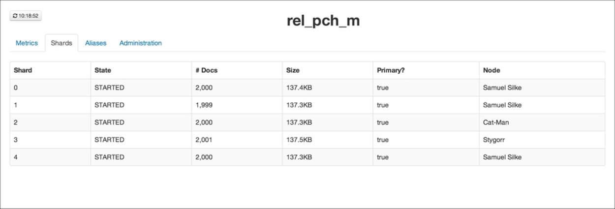
As we can see, the five shards of the index are located on three different nodes. Every shard has more or less the same number of documents. This is what we would expect—Elasticsearch used hashing to calculate the shard on which documents should be placed.
Now, let's look at the second index, which contains our children documents, as shown in the following screenshot:
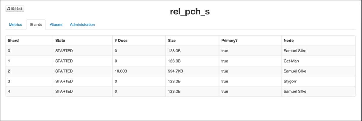
The situation is different. We still have five shards, but four of them are empty and the last one contains all the 10,000 documents! So something is not right—all the documents we indexed are located in one particular shard. This is because Elasticsearch will always put documents with the same parent in the same shard (in other words, the routing parameter value for children documents is always equal to the parent parameter value). Our example shows that in situations when some parent documents have substantially more children, we can end up with uneven shards, which may cause performance and storage issues—for example, some shards may be idling, while others will be constantly overloaded.
A few words about alternatives
As we have seen, the handling of relations between documents can cause different problems to Elasticsearch. Of course, this is not only the case with Elasticsearch because full text search solutions are extremely valuable for searching and data analysis, and not for modeling relationships between data. If it is a big problem for your application, and the full text capability is not a core part of it, you may consider using an SQL database that allows full text searching to some extent. Of course, these solutions won't be as flexible and fast as Elasticsearch, but we have to pay the price if we need full relationship support. However, in most other cases, the change of data architecture and the elimination of relations by de-normalization will be sufficient.
Scripting changes between Elasticsearch versions
One of the great things in Elasticsearch is its scripting capabilities. You can use script for calculating score, text-based scoring, data filtering, and data analysis. Although scripting can be slow in some cases, such as calculating the score for each document, we think that this part of Elasticsearch is important. Because of this, we decided that this section should bring you the information about the changes and will extend the information present in the Elasticsearch Server Second Edition book.
Scripting changes
Elasticsearch scripting has gone through a lot of refactoring in version 1.0 and in the versions that came after that. Because of those changes, some users were lost as to why their scripts stopped working when upgrading to version 1.2 of Elasticsearch and what is happening in general. This section will try to give you an insight on what to expect.
Security issues
During the lifetime of Elasticsearch 1.1, an exploit was published (see http://bouk.co/blog/elasticsearch-rce/): it showed that with the default configuration, Elasticsearch was not fully secure. Because of that, dynamic scripting was disabled by default in Elasticsearch 1.2. Although, disabling dynamic scripting was enough to make Elasticsearch secure, it made script usage far more complicated.
Groovy – the new default scripting language
With the release of Elasticsearch 1.3, we can use a new scripting language that will become default in the next version: Groovy (see http://groovy.codehaus.org/). The reason for this is that it can be closed in its own sandbox, preventing dynamic scripts from doing any harm to the cluster and the operating system. In addition to that, because Groovy can be sandboxed, Elasticsearch allows us to use dynamic scripting when using it. Generally speaking, starting from version 1.3, if a scripting language can be sandboxed, it can be used in dynamic scripts. However, Groovy is not everything: Elasticsearch 1.3 allows us to use Lucene expressions, which we will cover in this section. However, with the release of Elasticsearch 1.3.8 and 1.4.3 dynamic scripting was turned off even for Groovy. Because of that, if you still want to use dynamic scripting for Groovy you need to add script.groovy.sandbox.enabled property to elasticsearch.yml and set it to true or make your Elasticsearch a bit less dynamic with stored scripts. Please be aware that enabling dynamic scripting exposes security issues though and should be used with caution.
Removal of MVEL language
Because of the security issues and introduction of Groovy, starting from Elasticsearch 1.4, MVEL will no longer be available by default with Elasticsearch distribution. The default language will be Groovy, and MVEL will only be available as a plugin installed on demand. Remember that if you want to drop MVEL scripts, it is really easy to port them to Groovy. Of course, you will be able to install the MVEL plugin, but still dynamic scripting will be forbidden.
Short Groovy introduction
Groovy is a dynamic language for the Java Virtual Machine. It was built on top of Java, with some inspiration from languages such as Python, Ruby, or Smalltalk. Even though Groovy is out of the context of this book, we decided to describe it because, as you know, it is the default scripting language starting from Elasticsearch 1.4. If you already know Groovy and you know how to use it in Elasticsearch, you can easily skip this section and move to the Scripting in full text context section of this book.
Note
The thing to remember is that Groovy is only sandboxed up to Elasticsearch 1.3.8 and 1.4.3. Starting from the mentioned versions it is not possible to run dynamic Groovy scripts unless Elasticsearch is configured to allow such. All the queries in the examples that we will show next require you to add script.groovy.sandbox.enabled property to elasticsearch.yml and set it to true.
Using Groovy as your scripting language
Before we go into an introduction to Groovy, let's learn how to use it in Elasticsearch scripts. To do this, check the version you are using. If you are using Elasticsearch older than 1.4, you will need to add the lang property with the value groovy. For example:
curl -XGET 'localhost:9200/library/_search?pretty' -d '{
"fields" : [ "_id", "_score", "title" ],
"query" : {
"function_score" : {
"query" : {
"match_all" : {}
},
"script_score" : {
"lang" : "groovy",
"script" : "_index[\"title\"].docCount()"
}
}
}
}'
If you are using Elasticsearch 1.4 or newer, you can easily skip the scripting language definition because Elasticsearch will use Groovy by default.
Variable definition in scripts
Groovy allows us to define variables in scripts used in Elasticsearch. To define a new variable, we use the def keyword followed by the variable name and its value. For example, to define a variable named sum and assign an initial value of 0, to it we would use the following snippet of code:
def sum = 0
Of course, we are not only bound to simple variables definition. We can define lists, for example, a list of four values:
def listOfValues = [0, 1, 2, 3]
We can define a range of values, for example, from 0 to 9:
def rangeOfValues = 0..9
Finally, we can define maps:
def map = ['count':1, 'price':10, 'quantity': 12]
The preceding line of code will result in defining a map with three keys (count, price, and quantity) and three values corresponding to those keys (1, 10, and 12).
Conditionals
We are also allowed to use conditional statements in scripts. For example, we can use standard if - else if - else structures:
if (count > 1) {
return count
} else if (count == 1) {
return 1
} else {
return 0
}
We can use the ternary operator:
def isHigherThanZero = (count > 0) ? true : false
The preceding code will assign a true value to the isHigherThanZero variable if the count variable is higher than 0. Otherwise, the value assigned to the isHigherThanZero variable will be false.
Of course, we are also allowed to use standard switch statements that allow us to use an elegant way of choosing the execution path based on the value of the statement:
def isEqualToTenOrEleven = false;
switch (count) {
case 10:
isEqualToTenOrEleven = true
break
case 11:
isEqualToTenOrEleven = true
break
default:
isEqualToTenOrEleven = false
}
The preceding code will set the value of the isEqualToTenOrEleven variable to true if the count variable is equal to 10 or 11. Otherwise, the value of the isEqualToTenOrEleven variable will be set to false.
Loops
Of course, we can also use loops when using Elasticsearch scripts and Groovy as the language in which scripts are written. Let's start with the while loop that is going to be executed until the statement in the parenthesis is true:
def i = 2
def sum = 0
while (i > 0) {
sum = sum + i
i--
}
The preceding loop will be executed twice and ended. In the first iteration, the i variable will have the value of 2, which means that the i > 0 statement is true. In the second iteration, the value of the i variable will be 1, which again makes the i > 0 statement true. In the third iteration, the i variable will be 0, which will cause the while loop not to execute its body and exit.
We can also use the for loop, which you are probably familiar with if you've used programming languages before. For example, to iterate 10 times over the for loop body, we could use the following code:
def sum = 0
for ( i = 0; i < 10; i++) {
sum += i
}
We can also iterate over a range of values:
def sum = 0
for ( i in 0..9 ) {
sum += i
}
Or iterate over a list of values:
def sum = 0
for ( i in [0, 1, 2, 3, 4, 5, 6, 7, 8, 9] ) {
sum += i
}
If we have a map, we can iterate over its entries:
def map = ['quantity':2, 'value':1, 'count':3]
def sum = 0
for ( entry in map ) {
sum += entry.value
}
An example
Now after seeing some basics of Groovy, let's try to run an example script that will modify the score of our documents. We will implement the following algorithm for score calculation:
· if the year field holds the value lower than 1800, we will give the book a score of 1.0
· if the year field is between 1800 and 1900, we will give the book a score of 2.0
· the rest of the books should have the score equal to the value of the year field minus 1000
The query that does the preceding example looks as follows:
curl -XGET 'localhost:9200/library/_search?pretty' -d '{
"fields" : [ "_id", "_score", "title", "year" ],
"query" : {
"function_score" : {
"query" : {
"match_all" : {}
},
"script_score" : {
"lang" : "groovy",
"script" : "def year = doc[\"year\"].value; if (year < 1800) { return 1.0 } else if (year < 1900) { return 2.0 } else { return year - 1000 }"
}
}
}
}'
Note
You may have noticed that we've separated the def year = doc[\"year\"].value statement in the script from the rest of it using the ; character. We did it because we have the script in a single line and we need to tell Groovy where our assign statement ends and where another statement starts.
The result returned by Elasticsearch for the preceding query is as follows:
{
"took" : 4,
"timed_out" : false,
"_shards" : {
"total" : 5,
"successful" : 5,
"failed" : 0
},
"hits" : {
"total" : 6,
"max_score" : 961.0,
"hits" : [ {
"_index" : "library",
"_type" : "book",
"_id" : "2",
"_score" : 961.0,
"fields" : {
"title" : [ "Catch-22" ],
"year" : [ 1961 ],
"_id" : "2"
}
}, {
"_index" : "library",
"_type" : "book",
"_id" : "3",
"_score" : 936.0,
"fields" : {
"title" : [ "The Complete Sherlock Holmes" ],
"year" : [ 1936 ],
"_id" : "3"
}
}, {
"_index" : "library",
"_type" : "book",
"_id" : "1",
"_score" : 929.0,
"fields" : {
"title" : [ "All Quiet on the Western Front" ],
"year" : [ 1929 ],
"_id" : "1"
}
}, {
"_index" : "library",
"_type" : "book",
"_id" : "6",
"_score" : 904.0,
"fields" : {
"title" : [ "The Peasants" ],
"year" : [ 1904 ],
"_id" : "6"
}
}, {
"_index" : "library",
"_type" : "book",
"_id" : "4",
"_score" : 2.0,
"fields" : {
"title" : [ "Crime and Punishment" ],
"year" : [ 1886 ],
"_id" : "4"
}
}, {
"_index" : "library",
"_type" : "book",
"_id" : "5",
"_score" : 1.0,
"fields" : {
"title" : [ "The Sorrows of Young Werther" ],
"year" : [ 1774 ],
"_id" : "5"
}
} ]
}
}
As you can see, our script worked as we wanted it to.
There is more
Of course, the information we just gave is not a comprehensive guide to Groovy and was never intended to be one. Groovy is out of the scope of this book and we wanted to give you a glimpse of what to expect from it. If you are interested in Groovy and you want to extend your knowledge beyond what you just read, we suggest going to the official Groovy web page and reading the documentation available at http://groovy.codehaus.org/.
Scripting in full text context
Of course, scripts are not only about modifying the score on the basis of data. In addition to this, we can use full text-specific statistics in our scripts, such as document frequency or term frequency. Let's look at these possibilities.
Field-related information
The first text-related information we can use in scripts we would like to talk about is field-related statistics. The field-related information Elasticsearch allows us to use is as follows:
· _index['field_name'].docCount(): Number of documents that contain a given field. This statistic doesn't take deleted documents into consideration.
· _index['field_name'].sumttf(): Sum of the number of times all terms appear in all documents in a given field.
· _index['field_name'].sumdf(): Sum of document frequencies. This shows the sum of the number of times all terms appear in a given field in all documents.
Note
Please remember that the preceding information is given for a single shard, not for the whole index, so they may differ between shards.
For example, if we would like to give our documents a score equal to the number of documents having the title field living in a given shard, we could run the following query:
curl -XGET 'localhost:9200/library/_search?pretty' -d '{
"fields" : [ "_id", "_score", "title" ],
"query" : {
"function_score" : {
"query" : {
"match_all" : {}
},
"script_score" : {
"lang" : "groovy",
"script" : "_index[\"title\"].docCount()"
}
}
}
}'
If we would look at the response, we would see the following:
{
"took" : 3,
"timed_out" : false,
"_shards" : {
"total" : 5,
"successful" : 5,
"failed" : 0
},
"hits" : {
"total" : 6,
"max_score" : 2.0,
"hits" : [ {
"_index" : "library",
"_type" : "book",
"_id" : "1",
"_score" : 2.0,
"fields" : {
"title" : [ "All Quiet on the Western Front" ],
"_id" : "1"
}
}, {
"_index" : "library",
"_type" : "book",
"_id" : "6",
"_score" : 2.0,
"fields" : {
"title" : [ "The Peasants" ],
"_id" : "6"
}
}, {
"_index" : "library",
"_type" : "book",
"_id" : "4",
"_score" : 1.0,
"fields" : {
"title" : [ "Crime and Punishment" ],
"_id" : "4"
}
}, {
"_index" : "library",
"_type" : "book",
"_id" : "5",
"_score" : 1.0,
"fields" : {
"title" : [ "The Sorrows of Young Werther" ],
"_id" : "5"
}
}, {
"_index" : "library",
"_type" : "book",
"_id" : "2",
"_score" : 1.0,
"fields" : {
"title" : [ "Catch-22" ],
"_id" : "2"
}
}, {
"_index" : "library",
"_type" : "book",
"_id" : "3",
"_score" : 1.0,
"fields" : {
"title" : [ "The Complete Sherlock Holmes" ],
"_id" : "3"
}
} ]
}
}
As you can see, we have five documents that were queried to return the preceding results. The first two documents have a score of 2.0, which means that they are probably living in the same shard because the four remaining documents have a score of 1.0, which means that are alone in their shard.
Shard level information
The shard level information that we are allowed to use are as follows:
· _index.numDocs(): Number of documents in a shard
· _index.maxDoc(): Internal identifier of the maximum number of documents in a shard
· _index.numDeletedDocs(): Number of deleted documents in a given shard
Note
Please remember that the preceding information is given for a single shard, not for the whole index, so they may differ between shards.
For example, if we would like to sort documents on the basis of the highest internal identifier each shard has, we could send the following query:
curl -XGET 'localhost:9200/library/_search?pretty' -d '{
"fields" : [ "_id", "_score", "title" ],
"query" : {
"function_score" : {
"query" : {
"match_all" : {}
},
"script_score" : {
"lang" : "groovy",
"script" : "_index.maxDoc()"
}
}
}
}'
Of course, it doesn't make much sense to use those statistics alone, like we just did, but with addition to other text-related information, they can be very useful.
Term level information
The next type of information that we can use in scripts is term level information. Elasticsearch allows us to use the following:
· _index['field_name']['term'].df(): Returns the number of documents the term appears in a given field
· _index['field_name']['term'].ttf(): Returns the sum of the number of times a given term appears in all documents in a given field
· _index['field_name']['term'].tf(): Returns the information about the number of times a given term appears in a given field in a document
To give a good example of how we can use the preceding statistics, let's index two documents by using the following commands:
curl -XPOST 'localhost:9200/scripts/doc/1' -d '{"name":"This is a document"}'
curl -XPOST 'localhost:9200/scripts/doc/2' -d '{"name":"This is a second document after the first document"}'
Now, let's try filtering documents on the basis of how many times a given term appears in the name field. For example, let's match only those documents that have in the name field the document term appearing at least twice. To do this, we could run the following query:
curl -XGET 'localhost:9200/scripts/_search?pretty' -d '{
"query" : {
"filtered" : {
"query" : {
"match_all" : {}
},
"filter" : {
"script" : {
"lang" : "groovy",
"script": "_index[\"name\"][\"document\"].tf() > 1"
}
}
}
}
}'
The result of the query would be as follows:
{
"took" : 1,
"timed_out" : false,
"_shards" : {
"total" : 5,
"successful" : 5,
"failed" : 0
},
"hits" : {
"total" : 1,
"max_score" : 1.0,
"hits" : [ {
"_index" : "scripts",
"_type" : "doc",
"_id" : "2",
"_score" : 1.0,
"_source":{"name":"This is a second document after the first document"}
} ]
}
}
As we can see, Elasticsearch did exactly what we wanted.
More advanced term information
In addition to already presented information, we can also use term positions, offsets, and payloads in our scripts. To get those, we can use one the _index['field_name'].get('term', OPTION) expression, where OPTION is one of the following:
· _OFFSETS: Term offsets
· _PAYLOADS: Term payloads
· _POSITIONS: Term positions
Note
Please remember that the field you want to get offsets or positions for needs to have this enabled during indexing.
In addition to this, we can also use the _CACHE option. It allows us to iterate multiple times over all the term positions. Options can also be combined using the | operator; for example, if you would like to get term offsets and positions for the document term in the titlefield, you could use the following expression in your script:
_index['title'].get('document', _OFFSETS | _POSITIONS).
One thing to remember is that all the preceding options return an object called that, depending on the options we have chosen, contains the following information:
· startOffset: Start offset for the term
· endOffset: End offset for the term
· payload: Payload for the term
· payloadAsInt(value): Returns payload for the term converted to integer or the value in case the current position doesn't have a payload
· payloadAsFloat(value): Returns payload for the term converted to float or the value in case the current position doesn't have a payload
· payloadAsString(value): Returns payload for the term converted to string or the value in case the current position doesn't have a payload
· position: Position of a term
To illustrate an example, let's create a new index with the following mappings:
curl -XPOST 'localhost:9200/scripts2' -d '{
"mappings" : {
"doc" : {
"properties" : {
"name" : { "type" : "string", "index_options" : "offsets" }
}
}
}
}'
After this, we index two documents using the following commands:
curl -XPOST 'localhost:9200/scripts2/doc/1' -d '{"name":"This is the first document"}'
curl -XPOST 'localhost:9200/scripts2/doc/2' -d '{"name":"This is a second simple document"}'
Now, let's set the score of our documents to the sum of all the start positions for the document term in the name field. To do this, we run the following query:
curl -XGET 'localhost:9200/scripts2/_search?pretty' -d '{
"query" : {
"function_score" : {
"query" : {
"match_all" : {}
},
"script_score" : {
"lang" : "groovy",
"script": "def termInfo = _index[\"name\"].get(\"document\",_OFFSETS); def sum = 0; for (offset in termInfo) { sum += offset.startOffset; }; return sum;"
}
}
}
}'
The results returned by Elasticsearch would be as follows:
{
"took" : 3,
"timed_out" : false,
"_shards" : {
"total" : 5,
"successful" : 5,
"failed" : 0
},
"hits" : {
"total" : 2,
"max_score" : 24.0,
"hits" : [ {
"_index" : "scripts2",
"_type" : "doc",
"_id" : "2",
"_score" : 24.0,
"_source":{"name":"This is a second simple document"}
}, {
"_index" : "scripts2",
"_type" : "doc",
"_id" : "1",
"_score" : 18.0,
"_source":{"name":"This is the first document"}
} ]
}
}
As we can see, it works. If we look at the formatted script, we would see something like the following:
def termInfo = _index['name'].get('document',_OFFSETS);
def sum = 0;
for (offset in termInfo) {
sum += offset.startOffset;
};
return sum;
As you can see, it is nothing sophisticated. First, we get the information about the offsets in an object; next, we create a variable to hold our offsets sum. Then, we have a loop for all the offsets information (we can have multiple instances of offsets for different occurrences of the same term in a field) and, finally, we return the sum that makes our score for the document to be set to the returned value.
Note
In addition to all what we talked about in the preceding section, we are also able to get information about term vectors if we turned them on during indexing. To do that, we can use the _index.termVectors() expression, which will return Apache Lucene Fieldsobject instance. You can find more about the Fields object in Lucene Javadocs available at https://lucene.apache.org/core/4_9_0/core/org/apache/lucene/index/Fields.html.
Lucene expressions explained
Although marked as experimental, we decided to talk about it because this is a new and very good feature. The reason that makes Lucene expressions very handy is using them is very fast—their execution is as fast as native scripts, but yet they are like dynamic scripts with some limitations. This section will show you what you can do with Lucene expressions.
The basics
Lucene provides functionality to compile a JavaScript expression to a Java bytecode. This is how Lucene expressions work and this is why they are as fast as native Elasticsearch scripts. Lucene expressions can be used in the following Elasticsearch functionalities:
· Scripts responsible for sorting
· Aggregations that work on numeric fields
· In the function_score query in the script_score query
· In queries using script_fields
In addition to this, you have to remember that:
· Lucene expressions can be only used on numeric fields
· Stored fields can't be accessed using Lucene expressions
· Missing values for a field will be given a value of 0
· You can use _score to access the document score and doc['field_name'].value to access the value of a single valued numeric field in the document
· No loops are possible, only single statements
An example
Knowing the preceding information, we can try using Lucene expressions to modify the score of our documents. Let's get back to our library index and try to increase the score of the given document by 10% of the year it was originally released. To do this, we could run the following query:
curl -XGET 'localhost:9200/library/_search?pretty' -d '{
"fields" : [ "_id", "_score", "title" ],
"query" : {
"function_score" : {
"query" : {
"match_all" : {}
},
"script_score" : {
"lang" : "expression",
"script" : "_score + doc[\"year\"].value * percentage",
"params" : {
"percentage" : 0.1
}
}
}
}
}'
The query is very simple, but let's discuss its structure. First, we are using the match_all query wrapped in the function_score query because we want all documents to match and we want to use script for scoring. We are also setting the script language to expression(by setting the lang property to expression) to tell Elasticsearch that our script is a Lucene expressions script. Of course, we provide the script and we parameterize it, just like we would with any other script. The results of the preceding query look as follows:
{
"took" : 4,
"timed_out" : false,
"_shards" : {
"total" : 5,
"successful" : 5,
"failed" : 0
},
"hits" : {
"total" : 6,
"max_score" : 197.1,
"hits" : [ {
"_index" : "library",
"_type" : "book",
"_id" : "2",
"_score" : 197.1,
"fields" : {
"title" : [ "Catch-22" ],
"_id" : "2"
}
}, {
"_index" : "library",
"_type" : "book",
"_id" : "3",
"_score" : 194.6,
"fields" : {
"title" : [ "The Complete Sherlock Holmes" ],
"_id" : "3"
}
}, {
"_index" : "library",
"_type" : "book",
"_id" : "1",
"_score" : 193.9,
"fields" : {
"title" : [ "All Quiet on the Western Front" ],
"_id" : "1"
}
}, {
"_index" : "library",
"_type" : "book",
"_id" : "6",
"_score" : 191.4,
"fields" : {
"title" : [ "The Peasants" ],
"_id" : "6"
}
}, {
"_index" : "library",
"_type" : "book",
"_id" : "4",
"_score" : 189.6,
"fields" : {
"title" : [ "Crime and Punishment" ],
"_id" : "4"
}
}, {
"_index" : "library",
"_type" : "book",
"_id" : "5",
"_score" : 178.4,
"fields" : {
"title" : [ "The Sorrows of Young Werther" ],
"_id" : "5"
}
} ]
}
}
As we can see, Elasticsearch did what it was asked to do.
There is more
Of course, the provided example is a very simple one. If you are interested in what Lucene expressions provide, please visit the official Javadocs available at http://lucene.apache.org/core/4_9_0/expressions/index.html?org/apache/lucene/expressions/js/package-summary.html. The documents available at the given URL provide more information about what Lucene exposes in expressions module.
Summary
In this chapter, we extended our knowledge about query handling and data analysis. First of all, we discussed query rescore, which can help us when we need to recalculate the score of the top documents returned by a query. We also learned how to control multimatching queries. After that, we looked at two new aggregation types—one allowing us to get significant terms from a set of results and the other allowing documents grouping: a highly anticipated feature. We also discussed differences in relationship handling and approaches we can take when using Elasticsearch. Finally, we extended our knowledge about the Elasticsearch scripting module and we've learned what changes were introduced after Elasticsearch 1.0.
In the next chapter, we will try to improve our user query experience. We will start with user spelling mistakes and how Elasticsearch can help us by turning mistakes into good queries. We will also see what approaches we can take to handle user spelling mistake situations. After that, we will discuss improving query relevance on a given example. We will show you a query returning poor results and we will tune the query to match our needs.
All materials on the site are licensed Creative Commons Attribution-Sharealike 3.0 Unported CC BY-SA 3.0 & GNU Free Documentation License (GFDL)
If you are the copyright holder of any material contained on our site and intend to remove it, please contact our site administrator for approval.
© 2016-2026 All site design rights belong to S.Y.A.