Mastering Elasticsearch, Second Edition (2015)
Chapter 5. The Index Distribution Architecture
In the previous chapter, we were focused on improving the user search experience. We started with using the terms and phrase suggester to correct typos in user queries. In addition to that, we used the completion suggester to create an efficient, index time-calculated autocomplete functionality. Finally, we saw what Elasticsearch tuning may look like. We started with a simple query; we added multi match queries, phrase queries, boosts, and used query slops. We saw how to filter our garbage results and how to improve phrase match importance. We used n-grams to avoid misspellings as an alternate method to using Elasticsearch suggesters. We also discussed how to use faceting to allow our users to narrow down search results and thus simplify the way in which they can find the desired documents or products. By the end of this chapter, we will have covered:
· Choosing the right amount of shards and replicas
· Routing
· Shard allocation behavior adjustments
· Using query execution preference
Choosing the right amount of shards and replicas
In the beginning, when you started using Elasticsearch, you probably began by creating the index, importing your data to it and, after that, you started sending queries. We are pretty sure all worked well—at least in the beginning when the amount of data and the number of queries per second were not high. In the background, Elasticsearch created some shards and probably replicas as well (if you are using the default configuration, for example), and you didn't pay much attention to this part of the deployment.
When your application grows, you have to index more and more data and handle more and more queries per second. This is the point where everything changes. Problems start to appear (you can read about how we can handle the application's growth in Chapter 8, Improving Performance). It's now time to think about how you should plan your index and its configuration to rise with your application. In this chapter, we will give you some guidelines on how to handle this. Unfortunately, there is no exact recipe; each application has different characteristics and requirements, based on which, not only does the index structure depend, but also the configuration. For example, these factors can be ones like the size of the document or the whole index, query types, and the desired throughput.
Sharding and overallocation
You already know from the Introducing Elasticsearch section in Chapter 1, Introduction to Elasticsearch, what sharding is, but let's recall it. Sharding is the splitting of an Elasticsearch index to a set of smaller indices, which allows us to spread them among multiple nodes in the same cluster. While querying, the result is a sum of all the results that were returned by each shard of an index (although it's not really a sum, because a single shard may hold all the data we are interested in). By default, Elasticsearch creates five shards for every index even in a single-node environment. This redundancy is called overallocation: it seems to be totally not needed at this point and only leads to more complexity when indexing (spreading document to shards) and handling queries (querying shards and merging the results). Happily, this complexity is handled automatically, but why does Elasticsearch do this?
Let's say that we have an index that is built only of a single shard. This means that if our application grows above the capacity of a single machine, we will face a problem. In the current version of Elasticsearch, there is no possibility of splitting the index into multiple, smaller parts: we need to say how many shards the index should be built of when we create that index. What we can do is prepare a new index with more shards and reindex the data. However, such an operation requires additional time and server resources, such as CPU time, RAM, and mass storage. When it comes to the production environment, we don't always have the required time and mentioned resources. On the other hand, while using overallocation, we can just add a new server with Elasticsearch installed, and Elasticsearch will rebalance the cluster by moving parts of the index to the new machine without the additional cost of reindexing. The default configuration (which means five shards and one replica) chosen by the authors of Elasticsearch is the balance between the possibilities of growing and overhead resulting from the need to merge results from a different shard.
The default shard number of five is chosen for standard use cases. So now, this question arises: when should we start with more shards or, on the contrary, try to keep the number of shards as low as possible?
The first answer is obvious. If you have a limited and strongly defined data set, you can use only a single shard. If you do not, however, the rule of thumb dictates that the optimal number of shards be dependent on the target number of nodes. So, if you plan to use 10 nodes in the future, you need to configure the index to have 10 shards. One important thing to remember is that for high availability and query throughput, we should also configure replicas, and it also takes up room on the nodes just like the normal shard. If you have one additional copy of each shard (number_of_replicas equal to one), you end up with 20 shards—10 with the main data and 10 with its replicas.
To sum up, our simple formula can be presented as follows:
![]()
In other words, if you have planned to use 10 shards and you like to have two replicas, the maximum number of nodes that will hold the data for this setup will be 30.
A positive example of overallocation
If you carefully read the previous part of this chapter, you will have a strong conviction that you should use the minimal number of shards. However, sometimes, having more shards is handy, because a shard is, in fact, an Apache Lucene index, and more shards means that every operation executed on a single, smaller Lucene index (especially indexing) will be faster. Sometimes, this is a good enough reason to use many shards. Of course, there is the possible cost of splitting a query into multiple requests to each and every shard and merge the response from it. This can be avoided for particular types of applications where the queries are always filtered by the concrete parameter. This is the case with multitenant systems, where every query is run in the context of the defined user. The idea is simple; we can index the data of this user in a single shard and use only that shard during querying. This is in place when routing should be used (we will discuss it in detail in the Routing explained section in this chapter).
Multiple shards versus multiple indices
You may wonder whether, if a shard is the de-facto of a small Lucene index, what about true Elasticsearch indices? What is the difference between having multiple small shards and having multiple indices? Technically, the difference is not that great and, for some use cases, having more than a single index is the right approach (for example, to store time-based data such as logs in time-sliced indices). When you are using a single index with many shards, you can limit your operations to a single shard when using routing, for example. When dealing with indices, you may choose which data you are interested in; for example, choose only a few of your time-based indices using the logs_2014-10-10,logs_2014-10-11,... notation. More differences can be spotted in the shard and index-balancing logic, although we can configure both balancing logics.
Replicas
While sharding lets us store more data than we can fit on a single node, replicas are there to handle increasing throughput and, of course, for high availability and fault tolerance. When a node with the primary shard is lost, Elasticsearch can promote one of the available replicas to be a new primary shard. In the default configuration, Elasticsearch creates a single replica for each of the shards in the index. However, the number of replicas can be changed at any time using the Settings API. This is very convenient when we are at a point where we need more query throughput; increasing the number of replicas allows us to spread the querying load on more machine, which basically allows us to handle more parallel queries.
The drawback of using more replicas is obvious: the cost of additional space used by additional copies of each shard, the cost of indexing on nodes that host the replicas, and, of course, the cost of data copy between the primary shard and all the replicas. While choosing the number of shards, you should also consider how many replicas need to be present. If you select too many replicas, you can end up using disk space and Elasticsearch resources, when in fact, they won't be used. On the other hand, choosing to have none of the replicas may result in the data being lost if something bad happens to the primary shard.
Routing explained
In the Choosing the right amount of shards and replicas section in this chapter, we mentioned routing as a solution for the shards on which queries will be executed on a single one. Now it's time to look closer at this functionality.
Shards and data
Usually, it is not important how Elasticsearch divides data into shards and which shard holds the particular document. During query time, the query will be sent to all the shards of a particular index, so the only crucial thing is to use the algorithm that spreads our data evenly so that each shard contains similar amounts of data. We don't want one shard to hold 99 percent of the data while the other shard holds the rest—it is not efficient.
The situation complicates slightly when we want to remove or add a newer version of the document. Elasticsearch must be able to determine which shard should be updated. Although it may seem troublesome, in practice, it is not a huge problem. It is enough to use the sharding algorithm, which will always generate the same value for the same document identifier. If we have such an algorithm, Elasticsearch will know which shard to point to when dealing with a document.
However, there are times when it would be nice to be able to hit the same shard for some portion of data. For example, we would like to store every book of a particular type only on a particular shard and, while searching for that kind of book, we could avoid searching on many shards and merging results from them. Instead, because we know the value we used for routing, we could point Elasticsearch to the same shard we used during indexing. This is exactly what routing does. It allows us to provide information that will be used by Elasticsearch to determine which shard should be used for document storage and for querying; the same routing value will always result in the same shard. It's basically something like saying "search for documents on the shard where you've put the documents by using the provided routing value".
Let's test routing
To show you an example that will illustrate how Elasticsearch allocates shards and which documents are placed on the particular shard, we will use an additional plugin. It will help us visualize what Elasticsearch did with our data. Let's install the Paramedic plugin using the following command:
bin/plugin -install karmi/elasticsearch-paramedic
After restarting Elasticsearch, we can point our browser to http://localhost:9200/_plugin/paramedic/index.html and we will able to see a page with various statistics and information about indices. For our example, the most interesting information is the cluster color that indicates the cluster state and the list of shards and replicas next to every index.
Let's start two Elasticsearch nodes and create an index by running the following command:
curl -XPUT 'localhost:9200/documents' -d '{
"settings": {
"number_of_replicas": 0,
"number_of_shards": 2
}
}'
We've created an index without replicas, which is built of two shards. This means that the largest cluster can have only two nodes, and each next node cannot be filled with data unless we increase the number of replicas (you can read about this in the Choosing the right amount of shards and replicas section of this chapter). The next operation is to index some documents; we will do that by using the following commands:
curl -XPUT localhost:9200/documents/doc/1 -d '{ "title" : "Document No. 1" }'
curl -XPUT localhost:9200/documents/doc/2 -d '{ "title" : "Document No. 2" }'
curl -XPUT localhost:9200/documents/doc/3 -d '{ "title" : "Document No. 3" }'
curl -XPUT localhost:9200/documents/doc/4 -d '{ "title" : "Document No. 4" }'
After that, if we would look at the installed Paramedic plugin, we would see our two primary shards created and assigned.
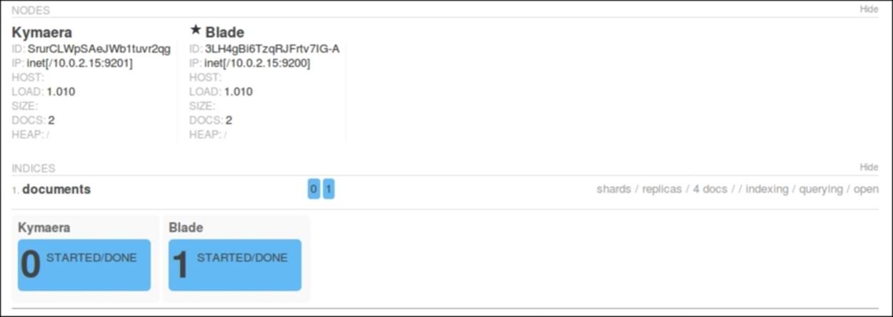
In the information about nodes, we can also find the information that we are currently interested in. Each of the nodes in the cluster holds exactly two documents. This leads us to the conclusion that the sharding algorithm did its work perfectly, and we have an index that is built of shards that have evenly redistributed documents.
Now, let's create some chaos and let's shut down the second node. Now, using Paramedic, we should see something like this:
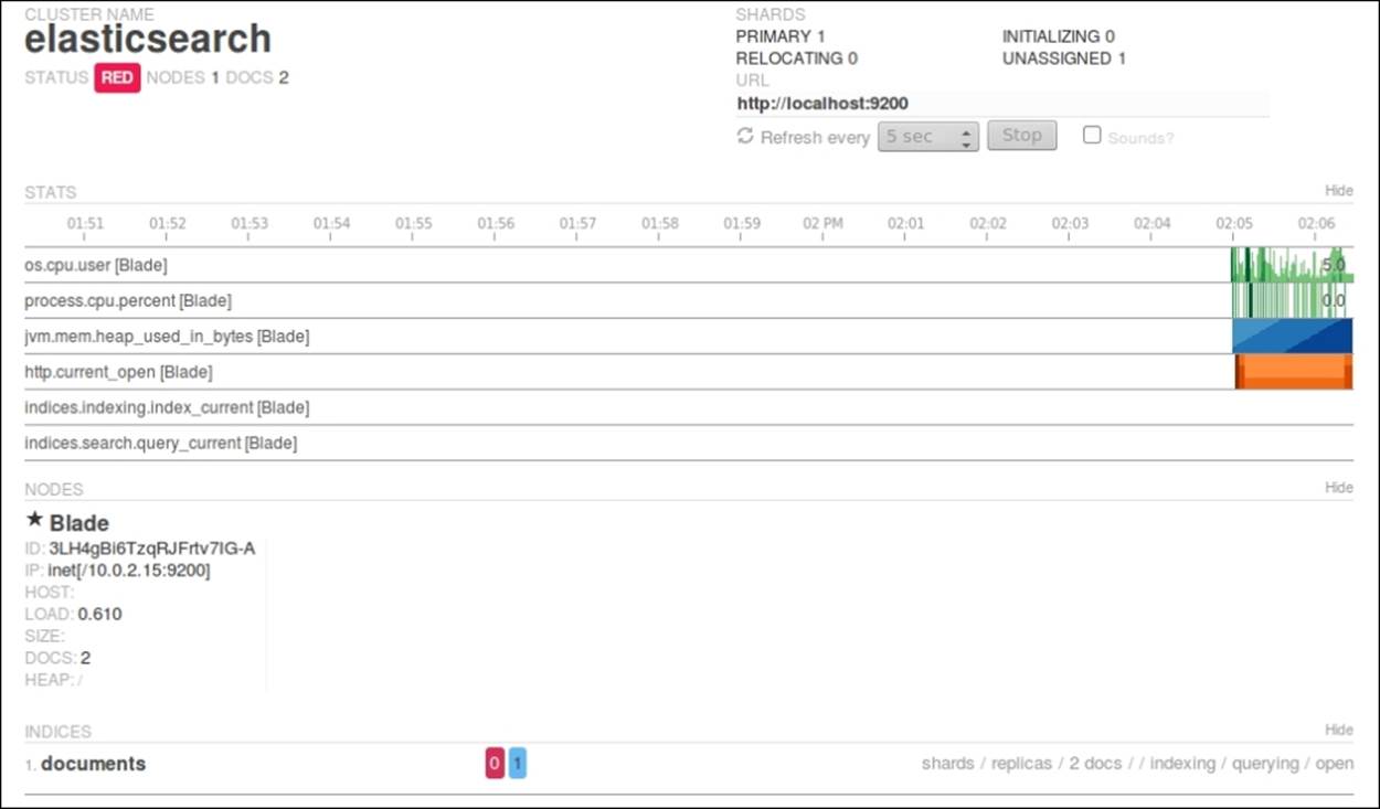
The first information we see is that the cluster is now in the red state. This means that at least one primary shard is missing, which tells us that some of the data is not available and some parts of the index are not available. Nevertheless, Elasticsearch allows us toexecute queries; it is our decision as to what applications should do—inform the user about the possibility of incomplete results or block querying attempts. Let's try to run a simple query by using the following command:
curl -XGET 'localhost:9200/documents/_search?pretty'
The response returned by Elasticsearch will look as follows:
{
"took" : 26,
"timed_out" : false,
"_shards" : {
"total" : 2,
"successful" : 1,
"failed" : 0
},
"hits" : {
"total" : 2,
"max_score" : 1.0,
"hits" : [ {
"_index" : "documents",
"_type" : "doc",
"_id" : "2",
"_score" : 1.0,
"_source":{ "title" : "Document No. 2" }
}, {
"_index" : "documents",
"_type" : "doc",
"_id" : "4",
"_score" : 1.0,
"_source":{ "title" : "Document No. 4" }
} ]
}
}
As you can see, Elasticsearch returned the information about failures; we can see that one of the shards is not available. In the returned result set, we can only see the documents with identifiers of 2 and 4. Other documents have been lost, at least until the failed primary shard is back online. If you start the second node, after a while (depending on the network and gateway module settings), the cluster should return to the green state and all documents should be available. Now, we will try to do the same using routing, and we will try to observe the difference in the Elasticsearch behavior.
Indexing with routing
With routing, we can control the target shard Elasticsearch will choose to send the documents to by specifying the routing parameter. The value of the routing parameter is irrelevant; you can use whatever value you choose. The important thing is that the same value of the routing parameter should be used to place different documents together in the same shard. To say it simply, using the same routing value for different documents will ensure us that these documents will be placed in the same shard.
There are a few possibilities as to how we can provide the routing information to Elasticsearch. The simplest way is add the routing URI parameter when indexing a document, for example:
curl -XPUT localhost:9200/books/doc/1?routing=A -d '{ "title" : "Document" }'
Of course, we can also provide the routing value when using bulk indexing. In such cases, routing is given in the metadata for each document by using the _routing property, for example:
curl -XPUT localhost:9200/_bulk --data-binary '
{ "index" : { "_index" : "books", "_type" : "doc", "_routing" : "A" }}
{ "title" : "Document" }
'
Another option is to place a _routing field inside the document. However, this will work properly only when the _routing field is defined in the mappings. For example, let's create an index called books_routing by using the following command:
curl -XPUT 'localhost:9200/books_routing' -d '{
"mappings": {
"doc": {
"_routing": {
"required": true,
"path": "_routing"
},
"properties": {
"title" : {"type": "string" }
}
}
}
}'
Now we can use _routing inside the document body, for example, like this:
curl -XPUT localhost:9200/books_routing/doc/1 -d '{ "title" : "Document", "_routing" : "A" }'
In the preceding example, we used a _routing field. It is worth mentioning that the path parameter can point to any field that's not analyzed from the document. This is a very powerful feature and one of the main advantages of the routing feature. For example, if we extend our document with the library_id field's indicated library where the book is available, it is logical that all queries based on library can be more effective when we set up routing based on this library_id field. However, you have to remember that getting the routing value from a field requires additional parsing.
Routing in practice
Now let's get back to our initial example and do the same as what we did but now using routing. The first thing is to delete the old documents. If we do not do this and add documents with the same identifier, routing may cause that same document to now be placed in the other shard. Therefore, we run the following command to delete all the documents from our index:
curl -XDELETE 'localhost:9200/documents/_query?q=*:*'
After that, we index our data again, but this time, we add the routing information. The commands used to index our documents now look as follows:
curl -XPUT localhost:9200/documents/doc/1?routing=A -d '{ "title" : "Document No. 1" }'
curl -XPUT localhost:9200/documents/doc/2?routing=B -d '{ "title" : "Document No. 2" }'
curl -XPUT localhost:9200/documents/doc/3?routing=A -d '{ "title" : "Document No. 3" }'
curl -XPUT localhost:9200/documents/doc/4?routing=A -d '{ "title" : "Document No. 4" }'
As we said, the routing parameter tells Elasticsearch in which shard the document should be placed. Of course, it may happen that more than a single document will be placed in the same shard. That's because you usually have less shards than routing values. If we now kill one node, Paramedic will again show you the red cluster and the state. If we query for all the documents, Elasticsearch will return the following response (of course, it depends which node you kill):
curl -XGET 'localhost:9200/documents/_search?q=*&pretty'
The response from Elasticsearch would be as follows:
{
"took" : 24,
"timed_out" : false,
"_shards" : {
"total" : 2,
"successful" : 1,
"failed" : 0
},
"hits" : {
"total" : 3,
"max_score" : 1.0,
"hits" : [ {
"_index" : "documents",
"_type" : "doc",
"_id" : "1",
"_score" : 1.0,
"_source":{ "title" : "Document No. 1" }
}, {
"_index" : "documents",
"_type" : "doc",
"_id" : "3",
"_score" : 1.0,
"_source":{ "title" : "Document No. 3" }
}, {
"_index" : "documents",
"_type" : "doc",
"_id" : "4",
"_score" : 1.0,
"_source":{ "title" : "Document No. 4" }
} ]
}
}
In our case, the document with the identifier 2 is missing. We lost a node with the documents that had the routing value of B. If we were less lucky, we could lose three documents!
Querying
Routing allows us to tell Elasticsearch which shards should be used for querying. Why send queries to all the shards that build the index if we want to get data from a particular subset of the whole index? For example, to get the data from a shard where routing Awas used, we can run the following query:
curl -XGET 'localhost:9200/documents/_search?pretty&q=*&routing=A'
We just added a routing parameter with the value we are interested in. Elasticsearch replied with the following result:
{
"took" : 0,
"timed_out" : false,
"_shards" : {
"total" : 1,
"successful" : 1,
"failed" : 0
},
"hits" : {
"total" : 3,
"max_score" : 1.0,
"hits" : [ {
"_index" : "documents",
"_type" : "doc",
"_id" : "1",
"_score" : 1.0, "_source" : { "title" : "Document No. 1" }
}, {
"_index" : "documents",
"_type" : "doc",
"_id" : "3",
"_score" : 1.0, "_source" : { "title" : "Document No. 3" }
}, {
"_index" : "documents",
"_type" : "doc",
"_id" : "4",
"_score" : 1.0, "_source" : { "title" : "Document No. 4" }
} ]
}
}
Everything works like a charm. But look closer! We forgot to start the node that holds the shard with the documents that were indexed with the routing value of B. Even though we didn't have a full index view, the reply from Elasticsearch doesn't contain information about shard failures. This is proof that queries with routing hit only a chosen shard and ignore the rest. If we run the same query with routing=B, we will get an exception like the following one:
{
"error" : "SearchPhaseExecutionException[Failed to execute phase [query_fetch], all shards failed]",
"status" : 503
}
We can test the preceding behavior by using the Search Shard API. For example, let's run the following command:
curl -XGET 'localhost:9200/documents/_search_shards?pretty&routing=A' -d '{"query":"match_all":{}}'
The response from Elasticsearch would be as follows:
{
"nodes" : {
"QK5r_d5CSfaV1Wx78k633w" : {
"name" : "Western Kid",
"transport_address" : "inet[/10.0.2.15:9301]"
}
},
"shards" : [ [ {
"state" : "STARTED",
"primary" : true,
"node" : "QK5r_d5CSfaV1Wx78k633w",
"relocating_node" : null,
"shard" : 0,
"index" : "documents"
} ] ]
}
As we can see, only a single node will be queried.
There is one important thing that we would like to repeat. Routing ensures us that, during indexing, documents with the same routing value are indexed in the same shard. However, you need to remember that a given shard may have many documents with different routing values. Routing allows you to limit the number of shards used during queries, but it cannot replace filtering! This means that a query with routing and without routing should have the same set of filters. For example, if we use user identifiers as routing values if we search for that user's data, we should also include filters on that identifier.
Aliases
If you work as a search engine specialist, you probably want to hide some configuration details from programmers in order to allow them to work faster and not care about search details. In an ideal world, they should not worry about routing, shards, and replicas. Aliases allow us to use shards with routing as ordinary indices. For example, let's create an alias by running the following command:
curl -XPOST 'http://localhost:9200/_aliases' -d '{
"actions" : [
{
"add" : {
"index" : "documents",
"alias" : "documentsA",
"routing" : "A"
}
}
]
}'
In the preceding example, we created a named documentsA alias from the documents index. However, in addition to that, searching will be limited to the shard used when routing value A is used. Thanks to this approach, you can give information about the documentsAalias to developers, and they may use it for querying and indexing like any other index.
Multiple routing values
Elasticsearch gives us the possibility to search with several routing values in a single query. Depending on which shard documents with given routing values are placed, it could mean searching on one or more shards. Let's look at the following query:
curl -XGET 'localhost:9200/documents/_search?routing=A,B'
After executing it, Elasticsearch will send the search request to two shards in our index (which in our case, happens to be the whole index), because the routing value of A covers one of two shards of our index and the routing value of B covers the second shard of our index.
Of course, multiple routing values are supported in aliases as well. The following example shows you the usage of these features:
curl -XPOST 'http://localhost:9200/_aliases' -d '{
"actions" : [
{
"add" : {
"index" : "documents",
"alias" : "documentsA",
"search_routing" : "A,B",
"index_routing" : "A"
}
}
]
}'
The preceding example shows you two additional configuration parameters we didn't talk about until now—we can define different values of routing for searching and indexing. In the preceding case, we've defined that during querying (the search_routing parameter) two values of routing (A and B) will be applied. When indexing (index_routing parameter), only one value (A) will be used. Note that indexing doesn't support multiple routing values, and you should also remember proper filtering (you can add it to your alias).
Altering the default shard allocation behavior
In Elasticsearch Server Second Edition, published by Packt Publishing, we talked about a number of things related to the shard allocation functionality provided by Elasticsearch. We discussed the Cluster Reroute API, shard rebalancing, and shard awareness. Although now very commonly used, these topics are very important if you want to be in full control of your Elasticsearch cluster. Because of that, we decided to extend the examples provided in Elasticsearch Server Second Edition and provide you with guidance on how to use Elasticsearch shards awareness and alter the default shard allocation mechanism.
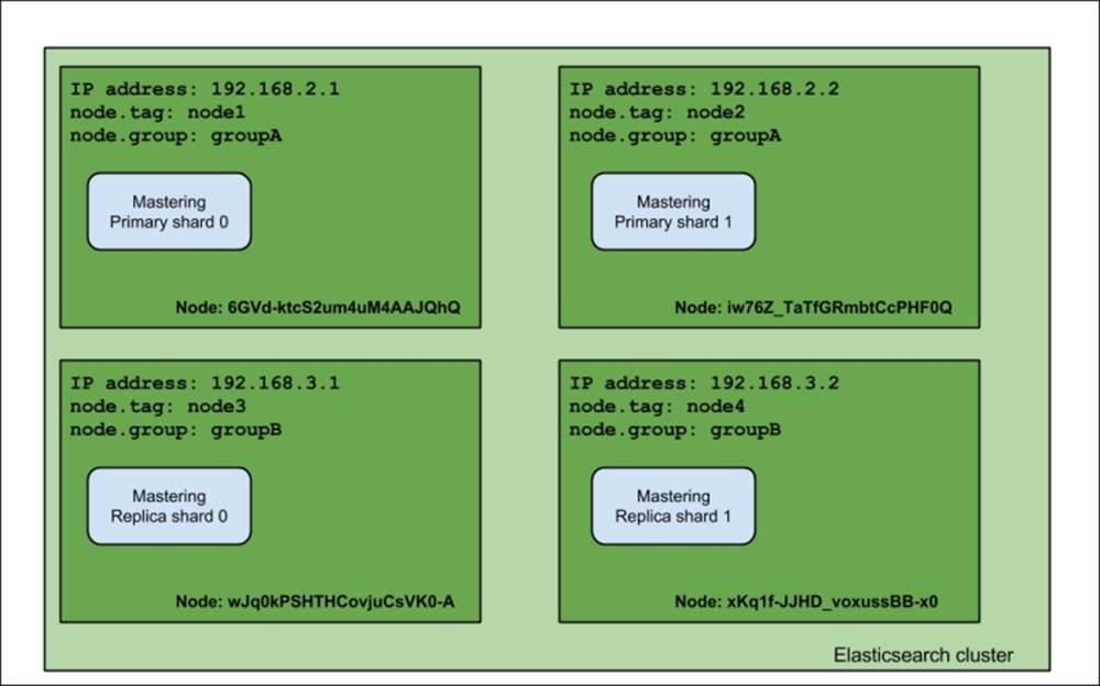
Let's start with a simple example. We assume that we have a cluster built of four nodes that looks as follows:
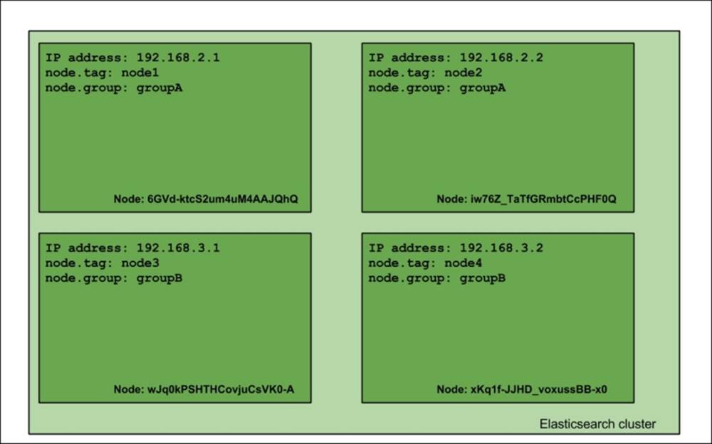
As you can see, our cluster is built of four nodes. Each node was bound to a specific IP address, and each node was given the tag property and a group property (added to elasticsearch.yml as node.tag and node.group properties). This cluster will serve the purpose of showing you how shard allocation filtering works. The group and tag properties can be given whatever names you want; you just need to prefix your desired property name with the node name; for example, if you would like to use a party property name, you would just add node.party: party1 to your elasticsearch.yml file.
Allocation awareness
Allocation awareness allows us to configure shards and their replicas' allocation with the use of generic parameters. In order to illustrate how allocation awareness works, we will use our example cluster. For the example to work, we should add the following property to the elasticsearch.yml file:
cluster.routing.allocation.awareness.attributes: group
This will tell Elasticsearch to use the node.group property as the awareness parameter.
Note
One can specify multiple attributes when setting the cluster.routing.allocation.awareness.attributes property, for example:
cluster.routing.allocation.awareness.attributes: group, node
After this, let's start the first two nodes, the ones with the node.group parameter equal to groupA, and let's create an index by running the following command:
curl -XPOST 'localhost:9200/mastering' -d '{
"settings" : {
"index" : {
"number_of_shards" : 2,
"number_of_replicas" : 1
}
}
}'
After this command, our two nodes' cluster will look more or less like this:
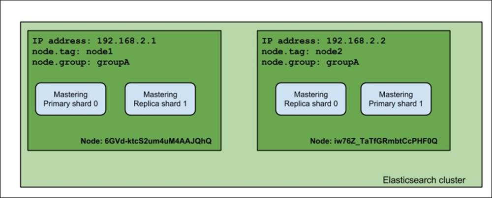
As you can see, the index was divided evenly between two nodes. Now let's see what happens when we launch the rest of the nodes (the ones with node.group set to groupB):
Notice the difference: the primary shards were not moved from their original allocation nodes, but the replica shards were moved to the nodes with a different node.group value. That's exactly right—when using shard allocation awareness, Elasticsearch won't allocate shards and replicas to the nodes with the same value of the property used to determine the allocation awareness (which, in our case, is node.group). One of the example usages of this functionality is to divide the cluster topology between virtual machines or physical locations in order to be sure that you don't have a single point of failure.
Note
Please remember that when using allocation awareness, shards will not be allocated to the node that doesn't have the expected attributes set. So, in our example, a node without the node.group property set will not be taken into consideration by the allocation mechanism.
Forcing allocation awareness
Forcing allocation awareness can come in handy when we know, in advance, how many values our awareness attributes can take, and we don't want more replicas than needed to be allocated in our cluster, for example, not to overload our cluster with too many replicas. To do this, we can force allocation awareness to be active only for certain attributes. We can specify these values using the cluster.routing.allocation.awareness.force.zone.values property and providing a list of comma-separated values to it. For example, if we would like allocation awareness to only use the groupA and groupB values of the node.group property, we would add the following to the elasticsearch.yml file:
cluster.routing.allocation.awareness.attributes: group
cluster.routing.allocation.awareness.force.zone.values: groupA, groupB
Filtering
Elasticsearch allows us to configure the allocation for the whole cluster or for the index level. In the case of cluster allocation, we can use the properties prefixes:
· cluster.routing.allocation.include
· cluster.routing.allocation.require
· cluster.routing.allocation.exclude
When it comes to index-specific allocation, we can use the following properties prefixes:
· index.routing.allocation.include
· index.routing.allocation.require
· index.routing.allocation.exclude
The previously mentioned prefixes can be used with the properties that we've defined in the elasticsearch.yml file (our tag and group properties) and with a special property called _ip that allows us to match or exclude IPs using nodes' IP address, for example, like this:
cluster.routing.allocation.include._ip: 192.168.2.1
If we would like to include nodes with a group property matching the groupA value, we would set the following property:
cluster.routing.allocation.include.group: groupA
Notice that we've used the cluster.routing.allocation.include prefix, and we've concatenated it with the name of the property, which is group in our case.
What include, exclude, and require mean
If you look closely at the parameters mentioned previously, you would notice that there are three kinds:
· include: This type will result in the inclusion of all the nodes with this parameter defined. If multiple include conditions are visible, then all the nodes that match at least one of these conditions will be taken into consideration when allocating shards. For example, if we would add two cluster.routing.allocation.include.tag parameters to our configuration, one with a property to the value of node1 and the second with the node2 value, we would end up with indices (actually, their shards) being allocated to the first and second node (counting from left to right). To sum up, the nodes that have the include allocation parameter type will be taken into consideration by Elasticsearch when choosing the nodes to place shards on, but that doesn't mean that Elasticsearch will put shards on them.
· require: This was introduced in the Elasticsearch 0.90 type of allocation filter, and it requires all the nodes to have the value that matches the value of this property. For example, if we would add one cluster.routing.allocation.require.tag parameter to our configuration with the value of node1 and a cluster.routing.allocation.require.group parameter, the value of groupA would end up with shards allocated only to the first node (the one with the IP address of 192.168.2.1).
· exclude: This allows us to exclude nodes with given properties from the allocation process. For example, if we set cluster.routing.allocation.include.tag to groupA, we would end up with indices being allocated only to nodes with IP addresses 192.168.3.1 and192.168.3.2 (the third and fourth node in our example).
Note
Property values can use simple wildcard characters. For example, if we would like to include all the nodes that have the group parameter value beginning with group, we could set the cluster.routing.allocation.include.group property to group*. In the example cluster case, it would result in matching nodes with the groupA and groupB group parameter values.
Runtime allocation updating
In addition to setting all discussed properties in the elasticsearch.yml file, we can also use the update API to update these settings in real-time when the cluster is already running.
Index level updates
In order to update settings for a given index (for example, our mastering index), we could run the following command:
curl -XPUT 'localhost:9200/mastering/_settings' -d '{
"index.routing.allocation.require.group": "groupA"
}'
As you can see, the command was sent to the _settings end-point for a given index. You can include multiple properties in a single call.
Cluster level updates
In order to update settings for the whole cluster, we could run the following command:
curl -XPUT 'localhost:9200/_cluster/settings' -d '{
"transient" : {
"cluster.routing.allocation.require.group": "groupA"
}
}'
As you can see, the command was sent to the cluster/_settings end-point. You can include multiple properties in a single call. Please remember that the transient name in the preceding command means that the property will be forgotten after the cluster restart. If you want to avoid this and set this property as a permanent one, use persistent instead of the transient one. An example command, which will keep the settings between restarts, could look like this:
curl -XPUT 'localhost:9200/_cluster/settings' -d '{
"persistent" : {
"cluster.routing.allocation.require.group": "groupA"
}
}'
Note
Please note that running the preceding commands, depending on the command and where your indices are located, can result in shards being moved between nodes.
Defining total shards allowed per node
In addition to the previously mentioned properties, we are also allowed to define how many shards (primaries and replicas) for an index can by allocated per node. In order to do that, one should set the index.routing.allocation.total_shards_per_node property to a desired value. For example, in elasticsearch.yml we could set this:
index.routing.allocation.total_shards_per_node: 4
This would result in a maximum of four shards per index being allocated to a single node.
This property can also be updated on a live cluster using the Update API, for example, like this:
curl -XPUT 'localhost:9200/mastering/_settings' -d '{
"index.routing.allocation.total_shards_per_node": "4"
}'
Now, let's see a few examples of what the cluster would look like when creating a single index and having the allocation properties used in the elasticsearch.yml file.
Defining total shards allowed per physical server
One of the properties that can be useful when having multiple nodes on a single physical server is cluster.routing.allocation.same_shard.host. When set to true, it prevents Elasticsearch from placing a primary shard and its replica (or replicas) on the same physical host. We really advise that you set this property to true if you have very powerful servers and that you go for multiple Elasticsearch nodes per physical server.
Inclusion
Now, let's use our example cluster to see how the allocation inclusion works. Let's start by deleting and recreating the mastering index by using the following commands:
curl -XDELETE 'localhost:9200/mastering'
curl -XPOST 'localhost:9200/mastering' -d '{
"settings" : {
"index" : {
"number_of_shards" : 2,
"number_of_replicas" : 0
}
}
}'
After this, let's try to run the following command:
curl -XPUT 'localhost:9200/mastering/_settings' -d '{
"index.routing.allocation.include.tag": "node1",
"index.routing.allocation.include.group": "groupA",
"index.routing.allocation.total_shards_per_node": 1
}'
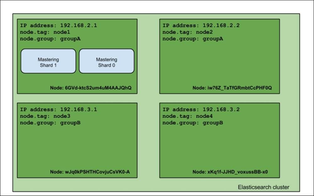
If we visualize the response of the index status, we would see that the cluster looks like the one in the following image:
As you can see, the mastering index shards are allocated to nodes with the tag property set to node1 or the group property set to groupA.
Requirement
Now, let's reuse our example cluster and try running the following command:
curl -XPUT 'localhost:9200/mastering/_settings' -d '{
"index.routing.allocation.require.tag": "node1",
"index.routing.allocation.require.group": "groupA"
}'
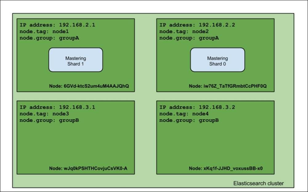
If we visualize the response of the index status command, we would see that the cluster looks like this:
As you can see, the view is different than the one when using include. This is because we tell Elasticsearch to allocate shards of the mastering index only to the nodes that match both the require parameters, and in our case, the only node that matches both is the first node.
Exclusion
Let's now look at exclusions. To test it, we try to run the following command:
curl -XPUT 'localhost:9200/mastering/_settings' -d '{
"index.routing.allocation.exclude.tag": "node1",
"index.routing.allocation.require.group": "groupA"
}'
Again, let's look at our cluster now:
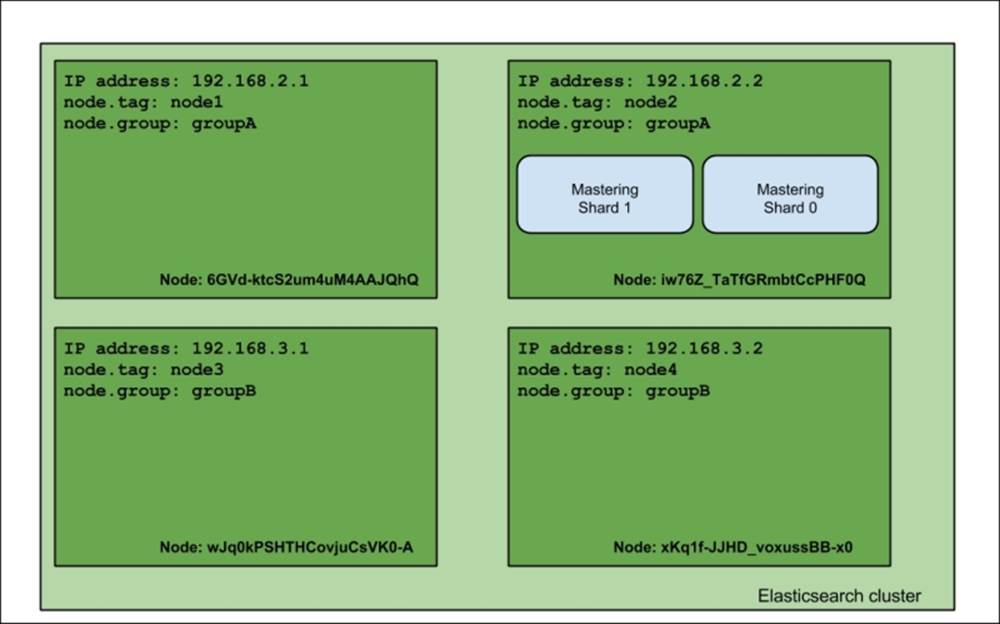
As you can see, we said that we require the group property to be equal to groupA, and we want to exclude the node with a tag equal to node1. This resulted in the shard of the mastering index being allocated to the node with the 192.168.2.2 IP address, which is what we wanted.
Disk-based allocation
Of course, the mentioned properties are not the only ones that can be used. With the release of Elasticsearch 1.3.0 we got the ability to configure awareness on the basis of the disk usage. By default, disk-based allocation is turned on, and if we want, we can turn it off by setting the cluster.routing.allocation.disk.threshold_enabled property to false.
There are three additional properties that can help us configure disk-based allocation. The cluster.routing.allocation.disk.watermark.low cluster controls when Elasticsearch does not allow you to allocate new shards on the node. By default, it is set to 85 percent and it means that when the disk usage is equal or higher than 85 percent, no new shards will be allocated on that node. The second property is cluster.routing.allocation.disk.watermark.high, which controls when Elasticsearch will try to move the shards out of the node and is set to 90 percent by default. This means that Elasticsearch will try to move the shard out of the node if the disk usage is 90 percent or higher.
Both cluster.routing.allocation.disk.watermark.low and cluster.routing.allocation.disk.watermark.high can be set to absolute values, for example, 1024mb.
Query execution preference
Let's forget about the shard placement and how to configure it—at least for a moment. In addition to all the fancy stuff that Elasticsearch allows us to set for shards and replicas, we also have the possibility to specify where our queries (and other operations, for example, the real-time GET) should be executed.
Before we get into the details, let's look at our example cluster:
As you can see, we have three nodes and a single index called mastering. Our index is divided into two primary shards, and there is one replica for each primary shard.
Introducing the preference parameter
In order to control where the query (and other operations) we are sending will be executed, we can use the preference parameter, which can be set to one of the following values:
· _primary: Using this property, the operations we are sending will only be executed on primary shards. So, if we send a query against mastering index with the preference parameter set to the _primary value, we would have it executed on the nodes with the names node1 and node2. For example, if you know that your primary shards are in one rack and the replicas are in other racks, you may want to execute the operation on primary shards to avoid network traffic.
· _primary_first: This option is similar to the _primary value's behavior but with a failover mechanism. If we ran a query against the mastering index with the preference parameter set to the _primary_first value, we would have it executed on the nodes with the names node1 and node2; however, if one (or more) of the primary shards fails, the query will be executed against the other shard, which in our case is allocated to a node named node3. As we said, this is very similar to the _primary value but with additional fallback to replicas if the primary shard is not available for some reason.
· _local: Elasticsearch will prefer to execute the operation on a local node, if possible. For example, if we send a query to node3 with the preference parameter set to _local, we would end up having that query executed on that node. However, if we send the same query to node2, we would end up with one query executed against the primary shard numbered 1 (which is located on that node) and the second part of the query will be executed against node1 or node3 where the shard numbered 0 resides. This is especially useful while trying to minimize the network latency; while using the _local preference, we ensure that our queries are executed locally whenever possible (for example, when running a client connection from a local node or sending a query to a node).
· _only_node:wJq0kPSHTHCovjuCsVK0-A: This operation will be only executed against a node with the provided identifier (which is wJq0kPSHTHCovjuCsVK0-A in this case). So in our case, the query would be executed against two replicas located on node3. Please remember that if there aren't enough shards to cover all the index data, the query will be executed against only the shard available in the specified node. For example, if we set the preference parameter to _only_node:6GVd-ktcS2um4uM4AAJQhQ, we would end up having our query executed against a single shard. This can be useful for examples where we know that one of our nodes is more powerful than the other ones and we want some of the queries to be executed only on that node.
· _prefer_node:wJq0kPSHTHCovjuCsVK0-A: This option sets the preference parameter to _prefer_node: the value followed by a node identifier (which is wJq0kPSHTHCovjuCsVK0-A in our case) will result in Elasticsearch preferring the mentioned node while executing the query, but if some shards are not available on the preferred node, Elasticsearch will send the appropriate query parts to nodes where the shards are available. Similar to the _only_node option, _prefer_node can be used while choosing a particular node, with a fall back to other nodes, however.
· _shards:0,1: This is the preference value that allows us to identify which shards the operation should be executed against (in our case, it will be all the shards, because we only have shards 0 and 1 in the mastering index). This is the only preference parameter value that can be combined with the other mentioned values. For example, in order to locally execute our query against the 0 and 1 shard, we should concatenate the 0,1 value with _local using the ; character, so the final value of the preference parameter should look like this: 0,1;_local. Allowing us to execute the operation against a single shard can be useful for diagnosis purposes.
· custom, string value: Setting the _preference parameter to a custom value will guarantee that the query with the same custom value will be executed against the same shards. For example, if we send a query with the _preference parameter set to themastering_elasticsearch value, we would end up having the query executed against primary shards located on nodes named node1 and node2. If we send another query with the same preference parameter value, then the second query will again be executed against the shards located on nodes named node1 and node2. This functionality can help us in cases where we have different refresh rates and we don't want our users to see different results while repeating requests. There is one more thing missing, which is the default behavior. What Elasticsearch will do by default is that it will randomize the operation between shards and replicas. If we sent many queries, we would end up having the same (or almost the same) number of queries run against each of the shards and replicas.
Summary
In this chapter, we talked about general shards and the index architecture. We chose the right amount of shards and replicas for our deployment, and we used routing during indexing and querying and in conjunction with aliases. We also discussed shard-allocation behavior adjustments, and finally, we looked at what query execution preference can bring us.
In the next chapter, we will take a deeper look, altering the Apache Lucene scoring mechanism by providing different similarity models. We will adjust our inverted index format by using codecs. We will discuss near real-time indexing and querying, flush and refresh operations, and transaction log configuration. We will talk about throttling and segment merges. Finally, we will discuss Elasticsearch caching—field data, filter, and query shard caches.
All materials on the site are licensed Creative Commons Attribution-Sharealike 3.0 Unported CC BY-SA 3.0 & GNU Free Documentation License (GFDL)
If you are the copyright holder of any material contained on our site and intend to remove it, please contact our site administrator for approval.
© 2016-2026 All site design rights belong to S.Y.A.