Mastering Elasticsearch, Second Edition (2015)
Chapter 8. Improving Performance
In the previous chapter, we looked at the discovery and recovery modules' configuration. We configured these modules and learned why they are important. We also saw additional discovery implementations available through plugins. We used the human-friendly Cat API to get information about the cluster in a human-readable form. We backed up our data to the external cloud storage, and we discussed tribe nodes—a federated search functionality allowing you to connect several Elasticsearch clusters together. By the end of this chapter, you will have learned the following things:
· What doc values can help us with when it comes to queries that are based on field data cache
· How garbage collector works
· How to benchmark your queries and fix performance problems before going to production
· What is the Hot Threads API and how it can help you with problems' diagnosis
· How to scale Elasticsearch and what to look at when doing that
· Preparing Elasticsearch for high querying throughput use cases
· Preparing Elasticsearch for high indexing throughput use cases
Using doc values to optimize your queries
In the Understanding Elasticsearch caching section of Chapter 6, Low-level Index Control we described caching: one of many ways that allow us to improve Elasticsearch's outstanding performance. Unfortunately, caching is not a silver bullet and, sometimes, it is better to avoid it. If your data is changing rapidly and your queries are very unique and not repeatable, then caching won't really help and can even make your performance worse sometimes.
The problem with field data cache
Every cache is based on a simple principle. The main assumption is that to improve performance, it is worth storing some part of the data in the memory instead of fetching from slow sources such as spinning disks, or to save the system a need to recalculate some processed data. However, caching is not free and it has its price—in terms of Elasticsearch, the cost of caching is mostly memory. Depending on the cache type, you may only need to store recently used data, but again, that's not always possible. Sometimes, it is necessary to hold all the information at once, because otherwise, the cache is just useless. For example, the field data cache used for sorting or aggregations—to make this functionality work, all values for a given field must be uninverted by Elasticsearch and placed in this cache. If we have a large number of documents and our shards are very large, we can be in trouble. The signs of such troubles may be something such as those in the response returned by Elasticsearch when running queries:
{
"error": "ReduceSearchPhaseException[Failed to execute phase [fetch], [reduce] ; shardFailures {[vWD3FNVoTy- 64r2vf6NwAw][dvt1][1]: ElasticsearchException[Java heap space]; nested: OutOfMemoryError[Java heap space]; }{[vWD3FNVoTy- 64r2vf6NwAw][dvt1][2]: ElasticsearchException[Java heap space]; nested: OutOfMemoryError[Java heap space]; }]; nested: OutOfMemoryError[Java heap space]; ",
"status": 500
}
The other indications of memory-related problems may be present in Elasticsearch logs and look as follows:
[2014-11-29 23:21:32,991][DEBUG][action.search.type ] [Abigail Brand] [dvt1][2], node[vWD3FNVoTy-64r2vf6NwAw], [P], s[STARTED]: Failed to execute [org.elasticsearch.action.search.SearchRequest@49d609d3] lastShard [true]
org.elasticsearch.ElasticsearchException: Java heap space
at org.elasticsearch.ExceptionsHelper.convertToRuntime (ExceptionsHelper.java:46)
at org.elasticsearch.search.SearchService.executeQueryPhase (SearchService.java:304)
at org.elasticsearch.search.action. SearchServiceTransportAction$5.call (SearchServiceTransportAction.java:231)
at org.elasticsearch.search.action. SearchServiceTransportAction$5.call (SearchServiceTransportAction.java:228)
at org.elasticsearch.search.action. SearchServiceTransportAction$23.run (SearchServiceTransportAction.java:559)
at java.util.concurrent.ThreadPoolExecutor.runWorker (ThreadPoolExecutor.java:1145)
at java.util.concurrent.ThreadPoolExecutor$Worker.run (ThreadPoolExecutor.java:615)
at java.lang.Thread.run(Thread.java:744)
Caused by: java.lang.OutOfMemoryError: Java heap space
This is where doc values can help us. Doc values are data structures in Lucene that are column-oriented, which means that they do not store the data in inverted index but keep them in a document-oriented data structure that is stored on the disk and calculated during the indexation. Because of this, doc values allow us to avoid keeping uninverted data in the field data cache and instead use doc values that access the data from the index, and since Elasticsearch 1.4.0, values are as fast as you would use in the memory field data cache.
The example of doc values usage
To show you the difference in memory consumption between the doc values-based approach and the field data cache-based approach, we indexed some simple documents into Elasticsearch. We indexed the same data to two indices: dvt1 and dvt2. Their structure is identical; the only difference is highlighted in the following code:
{
"t": {
"properties": {
"token": {
"type": "string",
"index": "not_analyzed",
"doc_values": true
}
}
}
}
The dvt2 index uses doc_values, while dtv1 doesn't use it, so the queries run against them (if they use sorting or aggregations) will use the field data cache.
Note
For the purpose of the tests, we've set the JVM heap lower than the default values given to Elasticsearch. The example Elasticsearch instance was run using:
bin/elasticsearch -Xmx16m -Xms16m
This seems somewhat insane for the first sight, but who said that we can't run Elasticsearch on the embedded device? The other way to simulate this problem is, of course, to index way more data. However, for the purpose of the test, keeping the memory low is more than enough.
Let's now see how Elasticsearch behaves when hitting our example indices. The query does not look complicated but shows the problem very well. We will try to sort our data on the basis of our single field in the document: the token type. As we know, sorting requires uninverted data, so it will use either the field data cache or doc values if they are available. The query itself looks as follows:
{
"sort": [
{
"token": {
"order": "desc"
}
}
]
}
It is a simple sort, but it is sufficient to take down our server when we try to search in the dvt1 index. At the same time, a query run against the dvt2 index returns the expected results without any sign of problems.
The difference in memory usage is significant. We can compare the memory usage for both indices after restarting Elasticsearch and removing the memory limit from the startup parameters. After running the query against both dvt1 and dvt2, we use the following command to check the memory usage:
curl -XGET 'localhost:9200/dvt1,dvt2/_stats/fielddata?pretty'
The response returned by Elasticsearch in our case was as follows:
{
"_shards" : {
"total" : 20,
"successful" : 10,
"failed" : 0
},
"_all" : {
"primaries" : {
"fielddata" : {
"memory_size_in_bytes" : 17321304,
"evictions" : 0
}
},
"total" : {
"fielddata" : {
"memory_size_in_bytes" : 17321304,
"evictions" : 0
}
}
},
"indices" : {
"dvt2" : {
"primaries" : {
"fielddata" : {
"memory_size_in_bytes" : 0,
"evictions" : 0
}
},
"total" : {
"fielddata" : {
"memory_size_in_bytes" : 0,
"evictions" : 0
}
}
},
"dvt1" : {
"primaries" : {
"fielddata" : {
"memory_size_in_bytes" : 17321304,
"evictions" : 0
}
},
"total" : {
"fielddata" : {
"memory_size_in_bytes" : 17321304,
"evictions" : 0
}
}
}
}
}
The most interesting parts are highlighted. As we can see, the indexes without doc_values use 17321304 bytes (16 MB) of memory for the field data cache. At the same time, the second index uses nothing; exactly no RAM memory is used to store the uninverted data.
Of course, as with most optimizations, doc values are not free to use when it comes to resources. Among the drawbacks of using doc values are speed—doc values are slightly slower compared to field data cache. The second drawback is the additional space needed for doc_values. For example, in our simple test case, the index with doc values was 41 MB, while the index without doc values was 34 MB. This gives us a bit more than 20 percent increase in the index size, but that usually depends on the data you have in your index. However, remember that if you have memory problems related to queries and field data cache, you may want to turn on doc values, reindex your data, and not worry about out-of-memory exceptions related to the field data cache anymore.
Knowing about garbage collector
You know that Elasticsearch is a Java application and, because of that, it runs in the Java Virtual Machine. Each Java application is compiled into a so-called byte code, which can be executed by the JVM. In the most general way of thinking, you can imagine that the JVM is just executing other programs and controlling their behavior. However, this is not what you will care about unless you develop plugins for Elasticsearch, which we will discuss in Chapter 9, Developing Elasticsearch Plugins. What you will care about is thegarbage collector—the piece of JVM that is responsible for memory management. When objects are de-referenced, they can be removed from the memory by the garbage collector. When the memory is running, the low garbage collector starts working and tries to remove objects that are no longer referenced. In this section, we will see how to configure the garbage collector, how to avoid memory swapping, how to log the garbage collector behavior, how to diagnose problems, and how to use some Java tools that will show you how it all works.
Note
You can learn more about the architecture of JVM in many places you find on the World Wide Web, for example, on Wikipedia: http://en.wikipedia.org/wiki/Java_virtual_machine.
Java memory
When we specify the amount of memory using the Xms and Xmx parameters (or the ES_MIN_MEM and ES_MAX_MEM properties), we specify the minimum and maximum size of the JVM heap space. It is basically a reserved space of physical memory that can be used by the Java program, which in our case, is Elasticsearch. A Java process will never use more heap memory than what we've specified with the Xmx parameter (or the ES_MAX_MEM property). When a new object is created in a Java application, it is placed in the heap memory. After it is no longer used, the garbage collector will try to remove that object from the heap to free the memory space and for JVM to be able to reuse it in the future. You can imagine that if you don't have enough heap memory for your application to create new objects on the heap, then bad things will happen. JVM will throw an OutOfMemory exception, which is a sign that something is wrong with the memory—either we don't have enough of it, or we have some memory leak and we don't release the object that we don't use.
Note
When running Elasticsearch on machines that are powerful and have a lot of free RAM memory, we may ask ourselves whether it is better to run a single large instance of Elasticsearch with plenty of RAM given to the JVM or a few instances with a smaller heap size. Before we answer this question, we need to remember that the more the heap memory is given to the JVM, the harder the work for the garbage collector itself gets. In addition to this, when setting the heap size to more than 31 GB, we don't benefit from the compressed operators, and JVM will need to use 64-bit pointers for the data, which means that we will use more memory to address the same amount of data. Given these facts, it is usually better to go for multiple smaller instances of Elasticsearch instead of one big instance.
The JVM memory (in Java 7) is divided into the following regions:
· eden space: This is the part of the heap memory where the JVM initially allocates most of the object types.
· survivor space: This is the part of the heap memory that stores objects that survived the garbage collection of the eden space heap. The survivor space is divided into survivor space 0 and survivor space 1.
· tenured generation: This is the part of the heap memory that holds objects that were living for some time in the survivor space heap part.
· permanent generation: This is the non-heap memory that stores all the data for the virtual machine itself, such as classes and methods for objects.
· code cache: This is the non-heap memory that is present in the HotSpot JVM that is used for the compilation and storage of native code.
The preceding classification can be simplified. The eden space and the survivor space is called the young generation heap space, and the tenured generation is often called old generation.
The life cycle of Java objects and garbage collections
In order to see how the garbage collector works, let's go through the life cycle of a sample Java object.
When a new object is created in a Java application, it is placed in the young generation heap space inside the eden space part. Then, when the next young generation garbage collection is run and the object survives that collection (basically, if it was not a one-time used object and the application still needs it), it will be moved to the survivor part of the young generation heap space (first to survivor 0 and then, after another young generation garbage collection, to survivor 1).
After living for sometime in the survivor 1 space, the object is moved to the tenured generation heap space, so it will now be a part of the old generation. From now on, the young generation garbage collector won't be able to move that object in the heap space. Now, this object will be live in the old generation until our application decides that it is not needed anymore. In such a case, when the next full garbage collection comes in, it will be removed from the heap space and will make place for new objects.
Note
There is one thing to remember: what you usually try to aim to do is smaller, but more garbage collections count rather than one but longer. This is because you want your application to be running at the same constant performance level and the garbage collector work to be transparent for Elasticsearch. When a big garbage collection happens, it can be a stop for the world garbage collection event, where Elasticsearch will be frozen for a short period of time, which will make your queries very slow and will stop your indexing process for some time.
Based on the preceding information, we can say (and it is actually true) that at least till now, Java used generational garbage collection; the more garbage collections our object survives, the further it gets promoted. Because of this, we can say that there are two types of garbage collectors working side by side: the young generation garbage collector (also called minor) and the old generation garbage collector (also called major).
Note
With the update 9 of Java 7, Oracle introduced a new garbage collector called G1. It is promised to be almost totally unaffected by stop the world events and should be working faster compared to other garbage collectors. To read more about G1, please refer tohttp://www.oracle.com/technetwork/tutorials/tutorials-1876574.html. Although Elasticsearch creators advise against using G1, numerous companies use it with success, and it allowed them to overcome problems with stop the world events when using Elasticsearch with large volumes of data and heavy queries.
Dealing with garbage collection problems
When dealing with garbage collection problems, the first thing you need to identify is the source of the problem. It is not straightforward work and usually requires some effort from the system administrator or the people responsible for handling the cluster. In this section, we will show you two methods of observing and identifying problems with the garbage collector; the first is to turn on logging for the garbage collector in Elasticsearch, and the second is to use the jstat command, which is present in most Java distributions.
In addition to the presented methods, please note that there are tools out there that can help you diagnose issues related to memory and the garbage collector. These tools are usually provided in the form of monitoring software solutions such as Sematext Group SPM (http://sematext.com/spm/index.html) or NewRelic (http://newrelic.com/). Such solutions provide sophisticated information not only related to garbage collection, but also the memory usage as a whole.
An example dashboard from the mentioned SPM application showing the garbage collector work looks as follows:
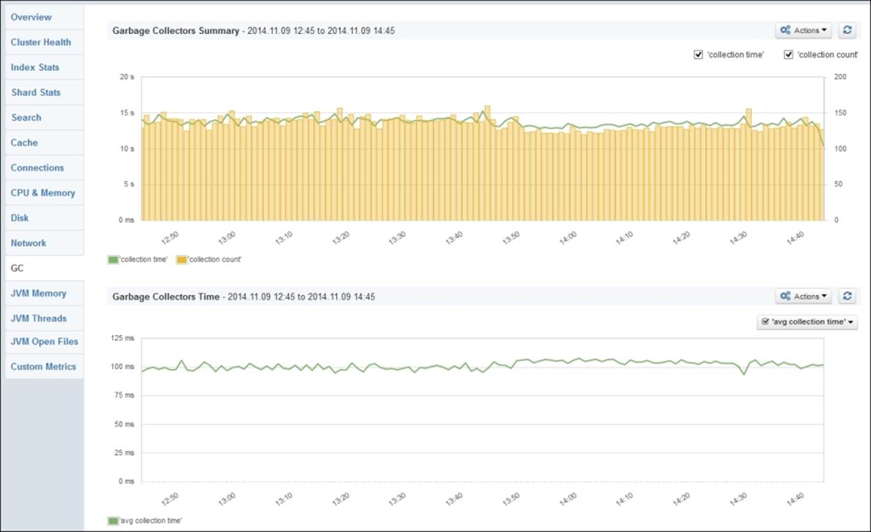
Turning on logging of garbage collection work
Elasticsearch allows us to observe periods when the garbage collector is working too long. In the default elasticsearch.yml configuration file, you can see the following entries, which are commented out by default:
monitor.jvm.gc.young.warn: 1000ms
monitor.jvm.gc.young.info: 700ms
monitor.jvm.gc.young.debug: 400ms
monitor.jvm.gc.old.warn: 10s
monitor.jvm.gc.old.info: 5s
monitor.jvm.gc.old.debug: 2s
As you can see, the configuration specifies three log levels and the thresholds for each of them. For example, for the info logging level, if the young generation collection takes 700 milliseconds or more, Elasticsearch will write the information to logs. In the case of the old generation, it will be written to logs if it will take more than five seconds.
Note
Please note that in older Elasticsearch versions (before 1.0), the prefix to log information related to young generation garbage collection was monitor.jvm.gc.ParNew.*, while the prefix to log old garbage collection information wasmonitor.jvm.gc.ConcurrentMarkSweep.*.
What you'll see in the logs is something like this:
[2014-11-09 15:22:52,355][WARN ][monitor.jvm ] [Lizard] [gc][old][964][1] duration [14.8s], collections [1]/[15.8s], total [14.8s]/[14.8s], memory [8.6gb]- >[3.4gb]/[11.9gb], all_pools {[Code Cache] [8.3mb]- >[8.3mb]/[48mb]}{[young] [13.3mb]->[3.2mb]/[266.2mb]}{[survivor] [29.5mb]->[0b]/[33.2mb]}{[old] [8.5gb]->[3.4gb]/[11.6gb]}
As you can see, the preceding line from the log file says that it is about the old garbage collector work. We can see that the total collection time took 14.8 seconds. Before the garbage collection operation, there was 8.6 GB of heap memory used (out of 11.9 GB). After the garbage collection work, the amount of heap memory used was reduced to 3.4 GB. After this, you can see information in more detailed statistics about which parts of the heap were taken into consideration by the garbage collector: the code cache, young generation space, survivor space, or old generation heap space.
When turning on the logging of the garbage collector work at a certain threshold, we can see when things don't run the way we would like by just looking at the logs. However, if you would like to see more, Java comes with a tool for that: jstat.
Using JStat
Running the jstat command to look at how our garbage collector works is as simple as running the following command:
jstat -gcutil 123456 2000 1000
The -gcutil switch tells the command to monitor the garbage collector work, 123456 is the virtual machine identifier on which Elasticsearch is running, 2000 is the interval in milliseconds between samples, and 1000 is the number of samples to be taken. So, in our case, the preceding command will run for a little more than 33 minutes (2000 * 1000 / 1000 / 60).
In most cases, the virtual machine identifier will be similar to your process ID or even the same but not always. In order to check which Java processes are running and what their virtual machines identifiers are, one can just run a jps command, which is provided with most JDK distributions. A sample command would be like this:
jps
The result would be as follows:
16232 Jps
11684 ElasticSearch
In the result of the jps command, we see that each line contains the JVM identifier, followed by the process name. If you want to learn more about the jps command, please refer to the Java documentation athttp://docs.oracle.com/javase/7/docs/technotes/tools/share/jps.html.
Note
Please remember to run the jstat command from the same account that Elasticsearch is running, or if that is not possible, run jstat with administrator privileges (for example, using the sudo command on Linux systems). It is crucial to have access rights to the process running Elasticsearch, or the jstat command won't be able to connect to that process.
Now, let's look at a sample output of the jstat command:
S0 S1 E O P YGC YGCT FGC FGCT GCT
12.44 0.00 27.20 9.49 96.70 78 0.176 5 0.495 0.672
12.44 0.00 62.16 9.49 96.70 78 0.176 5 0.495 0.672
12.44 0.00 83.97 9.49 96.70 78 0.176 5 0.495 0.672
0.00 7.74 0.00 9.51 96.70 79 0.177 5 0.495 0.673
0.00 7.74 23.37 9.51 96.70 79 0.177 5 0.495 0.673
0.00 7.74 43.82 9.51 96.70 79 0.177 5 0.495 0.673
0.00 7.74 58.11 9.51 96.71 79 0.177 5 0.495 0.673
The preceding example comes from the Java documentation and we decided to take it because it nicely shows us what jstat is all about. Let's start by saying what each of the columns mean:
· S0: This means that survivor space 0 utilization is a percentage of the space capacity
· S1: This means that survivor space 1 utilization is a percentage of the space capacity
· E: This means that the eden space utilization is a percentage of the space capacity
· O: This means that the old space utilization is a percentage of the space capacity
· YGC: This refers to the number of young garbage collection events
· YGCT: This is the time of young garbage collections in seconds
· FGC: This is the number of full garbage collections
· FGCT: This is the time of full garbage collections in seconds
· GCT: This is the total garbage collection time in seconds
Now, let's get back to our example. As you can see, there was a young garbage collection event after sample three and before sample four. We can see that the collection took 0.001 of a second (0.177 YGCT in the fourth sample minus 0.176 YGCT in the third sample). We also know that the collection promoted objects from the eden space (which is 0 percent in the fourth sample and was 83.97 percent in the third sample) to the old generation heap space (which was increased from 9.49 percent in the third sample to 9.51percent in the fourth sample). This example shows you how you can analyze the output of jstat. Of course, it can be time consuming and requires some knowledge about how garbage collector works, and what is stored in the heap. However, sometimes, it is the only way to see why Elasticsearch is stuck at certain moments.
Remember that if you ever see Elasticsearch not working correctly—the S0, S1 or E columns at 100 percent and the garbage collector working and not being able to handle these heap spaces—then either your young is too small and you should increase it (of course, if you have sufficient physical memory available), or you have run into some memory problems. These problems can be related to memory leaks when some resources are not releasing the unused memory. On the other hand, when your old generation space is at 100 percent and the garbage collector is struggling with releasing it (frequent garbage collections) but it can't, then it probably means that you just don't have enough heap space for your Elasticsearch node to operate properly. In such cases, what you can do without changing your index architecture is to increase the heap space that is available for the JVM that is running Elasticsearch (for more information about JVM parameters, refer to http://www.oracle.com/technetwork/java/javase/tech/vmoptions-jsp-140102.html).
Creating memory dumps
One additional thing that we didn't mention till now is the ability to dump the heap memory to a file. Java allows us to get a snapshot of the memory for a given point in time, and we can use that snapshot to analyze what is stored in the memory and find problems. In order to dump the Java process memory, one can use the jmap (http://docs.oracle.com/javase/7/docs/technotes/tools/share/jmap.html) command, for example, like this:
jmap -dump:file=heap.dump 123456
The 123456 heap dump, in our case, is the identifier of the Java process we want to get the memory dump for, and -dump:file=heap.dump specifies that we want the dump to be stored in the file named heap.dump. Such a dump can be further analyzed by specialized software, such as jhat (http://docs.oracle.com/javase/7/docs/technotes/tools/share/jhat.html), but the usage of such programs are beyond the scope of this book.
More information on the garbage collector work
Tuning garbage collection is not a simple process. The default options set for us in Elasticsearch deployment are usually sufficient for most cases, and the only thing you'll need to do is adjust the amount of memory for your nodes. The topic of tuning the garbage collector work is beyond the scope of the book; it is very broad and is called black magic by some developers. However, if you would like to read more about garbage collector, what the options are, and how they affect your application, I can suggest a great article that can be found at http://www.oracle.com/technetwork/java/javase/gc-tuning-6-140523.html. Although the article in the link is concentrated on Java 6, most of the options, if not all, can be successfully used with deployments running on Java 7.
Adjusting the garbage collector work in Elasticsearch
We now know how the garbage collector works and how to diagnose problems with it, so it would be nice to know how we can change Elasticsearch start up parameters to change how garbage collector works. It depends on how you run Elasticsearch. We will look at the two most common ones: standard start up script provided with the Elasticsearch distribution package and when using the service wrapper.
Using a standard start up script
When using a standard start up script in order to add additional JVM parameters, we should include them in the JAVA_OPTS environment property. For example, if we would like to include -XX:+UseParNewGC -XX:+UseConcMarkSweepGC in our Elasticsearch start up parameters in Linux-like systems, we would do the following:
export JAVA_OPTS="-XX:+UseParNewGC -XX:+UseConcMarkSweepGC"
In order to check whether the property was properly considered, we can just run another command:
echo $JAVA_OPTS
The preceding command should result in the following output in our case:
-XX:+UseParNewGC -XX:+UseConcMarkSweepGC
Service wrapper
Elasticsearch allows the user to install it as a service using the Java service wrapper (https://github.com/elasticsearch/elasticsearch-servicewrapper). If you are using the service wrapper, setting up JVM parameters is different when compared to the method shown previously. What we need to do is modify the elasticsearch.conf file, which will probably be located in /opt/elasticsearch/bin/service/ (if your Elasticsearch was installed in /opt/elasticsearch). In the mentioned file, you will see properties such as:
set.default.ES_HEAP_SIZE=1024
You will see properties such as these as well:
wrapper.java.additional.1=-Delasticsearch-service
wrapper.java.additional.2=-Des.path.home=%ES_HOME%
wrapper.java.additional.3=-Xss256k
wrapper.java.additional.4=-XX:+UseParNewGC
wrapper.java.additional.5=-XX:+UseConcMarkSweepGC
wrapper.java.additional.6=-XX:CMSInitiatingOccupancyFraction=75
wrapper.java.additional.7=-XX:+UseCMSInitiatingOccupancyOnly
wrapper.java.additional.8=-XX:+HeapDumpOnOutOfMemoryError
wrapper.java.additional.9=-Djava.awt.headless=true
The first property is responsible for setting the heap memory size for Elasticsearch, while the rest are additional JVM parameters. If you would like to add another parameter, you can just add another wrapper.java.additional property, followed by a dot and the next available number, for example:
wrapper.java.additional.10=-server
Note
One thing to remember is that tuning the garbage collector work is not something that you do once and forget. It requires experimenting, as it is very dependent on your data, queries and all that combined. Don't fear making changes when something is wrong, but also observe them and look how Elasticsearch works after making changes.
Avoid swapping on Unix-like systems
Although this is not strict about garbage collection and heap memory usage, we think that it is crucial to see how to disable swap. Swapping is the process of writing memory pages to the disk (swap partition in Unix-based systems) when the amount of physical memory is not sufficient or the operating system decides that for some reason, it is better to have some part of the RAM memory written into the disk. If the swapped memory pages will be needed again, the operating system will load them from the swap partition and allow processes to use them. As you can imagine, such processes take time and resources.
When using Elasticsearch, we want to avoid its process memory being swapped. You can imagine that having parts of memory used by Elasticsearch written to the disk and then again read from it can hurt the performance of both searching and indexing. Because of this, Elasticsearch allows us to turn off swapping for it. In order to do that, one should set bootstrap.mlockall to true in the elasticsearch.yml file.
However, the preceding setting is only the beginning. You also need to ensure that the JVM won't resize the heap by setting the Xmx and Xms parameters to the same values (you can do that by specifying the same values for the ES_MIN_MEM and ES_MAX_MEM environment variables for Elasticsearch). Also remember that you need to have enough physical memory to handle the settings you've set.
Now if we run Elasticsearch, we can run into the following message in the logs:
[2013-06-11 19:19:00,858][WARN ][common.jna ] Unknown mlockall error 0
This means that our memory locking is not working. So now, let's modify two files on our Linux operating system (this will require administration rights). We assume that the user who will run Elasticsearch is elasticsearch.
First, we modify /etc/security/limits.conf and add the following entries:
elasticsearch - nofile 64000
elasticsearch - memlock unlimited
The second thing is to modify the /etc/pam.d/common-session file and add the following:
session required pam_limits.so
After re-logging to the elasticsearch user account, you should be able to start Elasticsearch and not see the mlockall error message.
Benchmarking queries
There are a few important things when dealing with search or data analysis. We need the results to be precise, we need them to be relevant, and we need them to be returned as soon as possible. If you are a person responsible for designing queries that are run against Elasticsearch, sooner or later, you will find yourself in a position where you will need to improve the performance of your queries. The reasons can vary from hardware-based problems to bad data architecture to poor query design. When writing this book, the benchmark API was only available in the trunk of Elasticsearch, which means that it was not a part of official Elasticsearch distribution. For now we can either use tools like jMeter or ab (the Apache benchmark ishttp://httpd.apache.org/docs/2.2/programs/ab.html) or use trunk version of Elasticsearch. Please also note that the functionality we are describing can change with the final release, so keeping an eye onhttp://www.elasticsearch.org/guide/en/elasticsearch/reference/master/search-benchmark.html is a good idea if you want to use benchmarking functionality.
Preparing your cluster configuration for benchmarking
By default, the benchmarking functionality is disabled. Any attempt to use benchmarking on the Elasticsearch node that is not configured properly will lead to an error similar to the following one:
{
"error" : "BenchmarkNodeMissingException[No available nodes for executing benchmark [benchmark_name]]",
"status" : 503
}
This is okay; no one wants to take a risk of running potentially dangerous functionalities on production cluster. During performance testing and benchmarking, you will want to run many complicated and heavy queries, so running such benchmarks on the Elasticsearch cluster that is used by real users doesn't seem like a good idea. It will lead to the slowness of the cluster, and it could result in crashes and a bad user experience. To use benchmarking, you have to inform Elasticsearch which nodes can run the generated queries. Every instance we want to use for benchmarking should be run with the --node.bench option set to true. For example, we could run an Elasticsearch instance like this:
bin/elasticsearch --node.bench true
The other possibility is to add the node.bench property to the elasticsearch.yml file and, of course, set it to true. Whichever way we choose, we are now ready to run our first benchmark.
Running benchmarks
Elasticsearch provides the _bench REST endpoint, which allows you to define the task to run on benchmarking-enabled nodes in the cluster. Let's look at a simple example to learn how to do that. We will show you something practical; in the Handling filters and why it matters section in Chapter 2, Power User Query DSL, we talked about filtering. We tried to convince you that, in most cases, post filtering is bad. We can now check it ourselves and see whether the queries with post filtering are really slower. The command that allows us to test this looks as follows (we have used the Wikipedia database):
curl -XPUT 'localhost:9200/_bench/?pretty' -d '{
"name": "firstTest",
"competitors": [ {
"name": "post_filter",
"requests": [ {
"post_filter": {
"term": {
"link": "Toyota Corolla"
}
}
}]
},
{
"name": "filtered",
"requests": [ {
"query": {
"filtered": {
"query": {
"match_all": {}
},
"filter": {
"term": {
"link": "Toyota Corolla"
}
}
}
}
}]
}]
}'
The structure of a request to the _bench REST endpoint is pretty simple. It contains a list of competitors—queries or sets of queries (because each competitor can have more than a single query)—that will be compared to each other by the Elasticsearch benchmarking functionality. Each competitor has its name to allow easier results analysis. Now, let's finally look at the results returned by the preceding request:
{
"status": "COMPLETE",
"errors": [],
"competitors": {
"filtered": {
"summary": {
"nodes": [
"Free Spirit"
],
"total_iterations": 5,
"completed_iterations": 5,
"total_queries": 5000,
"concurrency": 5,
"multiplier": 1000,
"avg_warmup_time": 6,
"statistics": {
"min": 1,
"max": 5,
"mean": 1.9590000000000019,
"qps": 510.4645227156713,
"std_dev": 0.6143244085137575,
"millis_per_hit": 0.0009694501018329939,
"percentile_10": 1,
"percentile_25": 2,
"percentile_50": 2,
"percentile_75": 2,
"percentile_90": 3,
"percentile_99": 4
}
}
},
"post_filter": {
"summary": {
"nodes": [
"Free Spirit"
],
"total_iterations": 5,
"completed_iterations": 5,
"total_queries": 5000,
"concurrency": 5,
"multiplier": 1000,
"avg_warmup_time": 74,
"statistics": {
"min": 66,
"max": 217,
"mean": 120.88000000000022,
"qps": 8.272667107875579,
"std_dev": 18.487886855778815,
"millis_per_hit": 0.05085254582484725,
"percentile_10": 98,
"percentile_25": 109.26595744680851,
"percentile_50": 120.32258064516128,
"percentile_75": 131.3181818181818,
"percentile_90": 143,
"percentile_99": 171.01000000000022
}
}
}
}
}
As you can see, the test was successful; Elasticsearch returned an empty errors table. For every test we've run with both post_filter and filtered queries, only a single node named Free Spirit was used for benchmarking. In both cases, the same number of queries was used (5000) with the same number of simultaneous requests (5). Comparing the warm-up time and statistics, you can easily draw conclusions about which query is better. We would like to choose the filtered query; what about you?
Our example was quite simple (actually it was very simple), but it shows you the usefulness of benchmarking. Of course, our initial request didn't use all the configuration options exposed by the Elasticsearch benchmarking API. To summarize all the options, we've prepared a list of the available global options for the _bench REST endpoint:
· name: This is the name of the benchmark, making it easy to distinguish multiple benchmarks (refer to the Controlling currently run benchmarks section).
· competitors: This is the definition of tests that Elasticsearch should perform. It is the array of objects describing each test.
· num_executor_nodes: This is the maximum number of Elasticsearch nodes that will be used during query tests as a source of queries. It defaults to 1.
· percentiles: This is an array defining percentiles Elasticsearch should compute and return in results with the query execution time. The default value is [10, 25, 50, 75, 90, 99].
· iteration: This defaults to 5 and defines the number of repetitions for each competitor that Elasticsearch should perform.
· concurrency: This is the concurrency for each iteration and it defaults to 5, which means that five concurrent threads will be used by Elasticsearch.
· multiplier: This is the number of repetitions of each query in the given iteration. By default, the query is run 1000 times.
· warmup: This informs you that Elasticsearch should perform the warm-up of the query. By default, the warm-up is performed, which means that this value is set to true.
· clear_caches: By default, this is set to false, which means that before each iteration, Elasticsearch will not clean the caches. We can change this by setting the value to true. This parameter is connected with a series of parameters saying which cache should or should not be cleared. These additional parameters are clear_caches.filter (the filter cache), clear_caches.field_data (the field data cache), clear_caches.id (the ID cache), and clear_caches.recycler (the recycler cache). In addition, there are two parameters that can take an array of names: clear_caches.fields specifies the names of fields and which cache should be cleared and clear_caches.filter_keys specifies the names of filter keys to clear. For more information about caches, refer to the Understanding Elasticsearch caching section in Chapter 6, Low-level Index Control.
In addition to the global options, each competitor is an object that can contain the following parameters:
· name: Like its equivalent on the root level, this helps distinguish several competitors from each other.
· requests: This is a table of objects defining queries that should be run within given competitors. Each object is a standard Elasticsearch query that is defined using the query DSL.
· num_slowest: This is the number of the slowest queries tracked. It defaults to 1. If we want Elasticsearch to track and record more than one slow query, we should increase the value of that parameter.
· search_type: This indicates the type of searches that should be performed. Few of the options are query_then_fetch, dfs_query_then_fetch, and count. It defaults to query_then_fetch.
· indices: This is an array with indices names to which the queries should be limited.
· types: This is an array with type names to which the queries should be limited.
· iteration, concurrency, multiplier, warmup, clear_caches: These parameters override their version defined on the global level.
Controlling currently run benchmarks
Depending on the parameters we've used to execute our benchmark, a single benchmarking command containing several queries with thousands of repeats can run for several minutes or even hours. It is very handy to have a possibility to check how the tests run and estimate how long it will take for the benchmark command to end. As you can expect, Elasticsearch provides such information. To get this, the only thing we need to do is run the following command:
curl -XGET 'localhost:9200/_bench?pretty'
The output generated for the preceding command can look as follows (it was taken during the execution of our sample benchmark):
{
"active_benchmarks" : {
"firstTest" : {
"status" : "RUNNING",
"errors" : [ ],
"competitors" : {
"post_filter" : {
"summary" : {
"nodes" : [
"James Proudstar" ],
"total_iterations" : 5,
"completed_iterations" : 3,
"total_queries" : 3000,
"concurrency" : 5,
"multiplier" : 1000,
"avg_warmup_time" : 137.0,
"statistics" : {
"min" : 39,
"max" : 146,
"mean" : 78.95077720207264,
"qps" : 32.81378178835111,
"std_dev" : 17.42543552392229,
"millis_per_hit" : 0.031591310251188054,
"percentile_10" : 59.0,
"percentile_25" : 66.86363636363637,
"percentile_50" : 77.0,
"percentile_75" : 89.22727272727272,
"percentile_90" : 102.0,
"percentile_99" : 124.86000000000013
}
}
}
}
}
}
}
Thanks to it, you can see the progress of tests and try to estimate how long you will have to wait for the benchmark to finish and return the results. If you would like to abort the currently running benchmark (for example, it takes too long and you already see that the tested query is not optimal), Elasticsearch has a solution. For example, to abort our benchmark called firstTest, we run a POST request to the _bench/abort REST endpoint, just like this:
curl -XPOST 'localhost:9200/_bench/abort/firstTest?pretty'
The response returned by Elasticsearch will show you a partial result of the test. It is almost the same as what we've seen in the preceding example, except that the status of the benchmark will be set to ABORTED.
Very hot threads
When you are in trouble and your cluster works slower than usual and uses large amounts of CPU power, you know you need to do something to make it work again. This is the case when the Hot Threads API can give you the information necessary to find the root cause of problems. A hot thread in this case is a Java thread that uses a high CPU volume and executes for longer periods of time. Such a thread doesn't mean that there is something wrong with Elasticsearch itself; it gives you information on what can be a possible hotspot and allows you to see which part of your deployment you need to look more deeply at, such as query execution or Lucene segments merging. The Hot Threads API returns information about which parts of the Elasticsearch code are hot spots from the CPU side or where Elasticsearch is stuck for some reason.
When using the Hot Threads API, you can examine all nodes, a selected few of them, or a particular node using the /_nodes/hot_threads or /_nodes/{node or nodes}/hot_threads endpoints. For example, to look at hot threads on all the nodes, we would run the following command:
curl 'localhost:9200/_nodes/hot_threads'
The API supports the following parameters:
· threads (the default: 3): This is the number of threads that should be analyzed. Elasticsearch takes the specified number of the hottest threads by looking at the information determined by the type parameter.
· interval (the default: 500ms): Elasticsearch checks threads twice to calculate the percentage of time spent in a particular thread on an operation defined by the type parameter. We can use the interval parameter to define the time between these checks.
· type (the default: cpu): This is the type of thread state to be examined. The API can check the CPU time taken by the given thread (cpu), the time in the blocked state (block), or the time in the waiting (wait) state. If you would like to know more about the thread states, refer to http://docs.oracle.com/javase/7/docs/api/java/lang/Thread.State.html.
· snapshots (the default: 10): This is the number of stack traces (a nested sequence of method calls at a certain point of time) snapshots to take.
Using the Hot Threads API is very simple; for example, to look at hot threads on all the nodes that are in the waiting state with check intervals of one second, we would use the following command:
curl 'localhost:9200/_nodes/hot_threads?type=wait&interval=1s'
Usage clarification for the Hot Threads API
Unlike other Elasticsearch API responses where you can expect JSON to be returned, the Hot Threads API returns formatted text, which contains several sections. Before we discuss the response structure itself, we would like to tell you a bit about the logic that is responsible for generating this response. Elasticsearch takes all the running threads and collects various information about the CPU time spent in each thread, the number of times the particular thread was blocked or was in the waiting state, how long it was blocked or was in the waiting state, and so on. The next thing is to wait for a particular amount of time (specified by the interval parameter), and after that time passes, collect the same information again. After this is done, threads are sorted on the basis of time each particular thread was running. The sort is done in a descending order so that the threads running for the longest period of time are on top of the list. Of course, the mentioned time is measured for a given operation type specified by the type parameter. After this, the first N threads (where N is the number of threads specified by the threads parameter) are analyzed by Elasticsearch. What Elasticsearch does is that, at every few milliseconds, it takes a few snapshots (the number of snapshots is specified by the snapshotparameter) of stack traces of the threads that were selected in the previous step. The last thing that needs to be done is the grouping of stack traces in order to visualize changes in the thread state and return the response to the caller.
The Hot Threads API response
Now, let's go through the sections of the response returned by the Hot Threads API. For example, the following screenshot is a fragment of the Hot Threads API response generated for Elasticsearch that was just started:
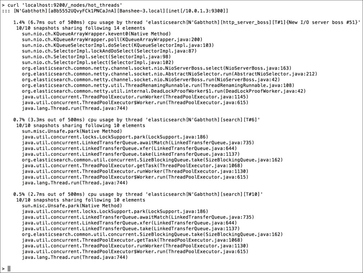
Now, let's discuss the sections of the response. To do that, we will use a slightly different response compared to the one shown previously. We do this to better visualize what is happening inside Elasticsearch. However, please remember that the general structure of the response will not change.
The first section of the Hot Threads API response shows us which node the thread is located on. For example, the first line of the response can look as follows:
::: [N'Gabthoth][aBb5552UQvyFCk1PNCaJnA][Banshee- 3.local][inet[/10.0.1.3:9300]]
Thanks to it, we can see which node the Hot Threads API returns information about and which node is very handy when the Hot Threads API call goes to many nodes.
The next lines of the Hot Threads API response can be divided into several sections, each starting with a line similar to the following one:
0.5% (2.7ms out of 500ms) cpu usage by thread 'elasticsearch[N'Gabthoth][search][T#10]'
In our case, we see a thread named search, which takes 0.5 percent of all the CPU time at the time when the measurement was done. The cpu usage part of the preceding line indicates that we are using type equal to cpu (other values you can expect here are block usage for threads in the blocked state and wait usage for threads in the waiting states). The thread name is very important here, because by looking at it, we can see which Elasticsearch functionality is the hot one. In our example, we see that this thread is all about searching (the search value). Other example values that you can expect to see are recovery_stream (for recovery module events), cache (for caching events), merge (for segments merging threads), index (for data indexing threads), and so on.
The next part of the Hot Threads API response is the section starting with the following information:
10/10 snapshots sharing following 10 elements
This information will be followed by a stack trace. In our case, 10/10 means that 10 snapshots have been taken for the same stack trace. In general, this means that all the examination time was spent in the same part of the Elasticsearch code.
Scaling Elasticsearch
As we already said multiple times both in this book and in Elasticsearch Server Second Edition, Elasticsearch is a highly scalable search and analytics platform. We can scale it both horizontally and vertically.
Vertical scaling
When we talk about vertical scaling, we often mean adding more resources to the server Elasticsearch is running on: we can add memory and we can switch to a machine with better CPU or faster disk storage. Of course, with better machines, we can expect increase in performance; depending on our deployment and its bottleneck, there can be smaller or higher improvement. However, there are limitations when it comes to vertical scaling. For example, one of such is the maximum amount of physical memory available for your servers or the total memory required by the JVM to operate. When you have large enough data and complicated queries, you can very soon run into memory issues, and adding new memory may not be helpful at all.
For example, you may not want to go beyond 31 GB of physical memory given to the JVM because of garbage collection and the inability to use compressed ops, which basically means that to address the same memory space, JVM will need to use twice the memory. Even though it seems like a very big issue, vertical scaling is not the only solution we have.
Horizontal scaling
The other solution available to us Elasticsearch users is horizontal scaling. To give you a comparison, vertical scaling is like building a sky scrapper, while horizontal scaling is like having many houses in a residential area. Instead of investing in hardware and having powerful machines, we choose to have multiple machines and our data split between them. Horizontal scaling gives us virtually unlimited scaling possibilities. Even with the most powerful hardware time, a single machine is not enough to handle the data, the queries, or both of them. If a single machine is not able to handle the amount of data, we have such cases where we divide our indices into multiple shards and spread them across the cluster, just like what is shown in the following figure:
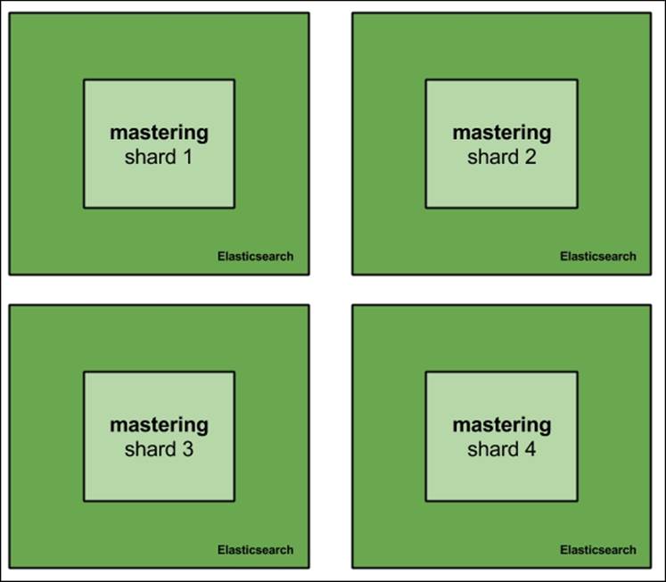
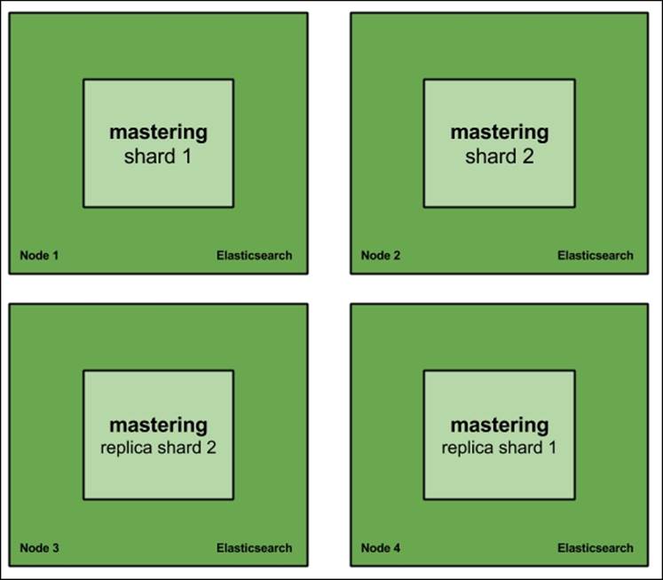
When we don't have enough processing power to handle queries, we can always create more replicas of the shards we have. We have our cluster: four Elasticsearch nodes with the mastering index created and running on it and built of four shards.
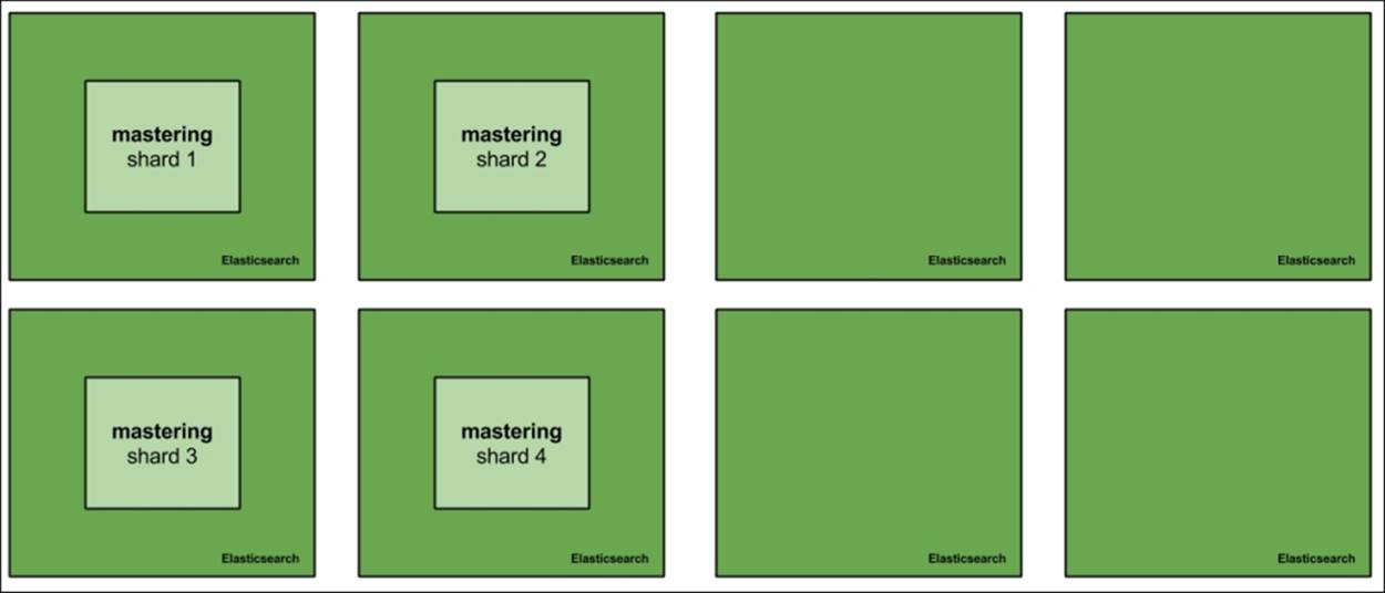
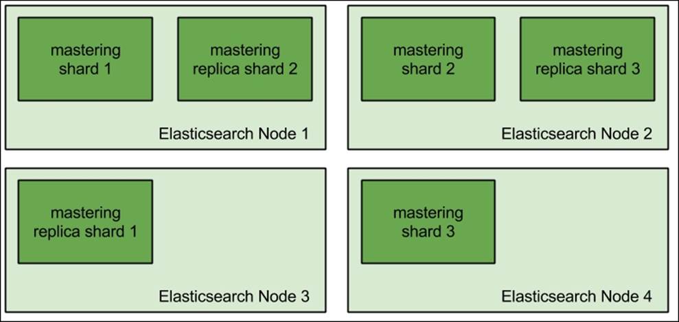
If we want to increase the querying capabilities of our cluster, we would just add additional nodes, for example, four of them. After adding new nodes to the cluster, we can either create new indices that will be built of more shards to spread the load more evenly, or add replicas to already existing shards. Both options are viable. We should go for more primary shards when our hardware is not enough to handle the amount of data it holds. In such cases, we usually run into out-of-memory situations, long shard query execution time, swapping, or high I/O waits. The second option—having replicas—is a way to go when our hardware is happily handling the data we have, but the traffic is so high that the nodes just can't keep up. The first option is simple, but let's look at the second case: having more replicas. So, with four additional nodes, our cluster would look as follows:
Now, let's run the following command to add a single replica:
curl -XPUT 'localhost:9200/mastering/_settings' -d '{
"index" : {
"number_of_replicas" : 1
}
}'
Our cluster view would look more or less as follows:
As you can see, each of the initial shards building the mastering index has a single replica stored on another node. Because of this, Elasticsearch is able to round robin the queries between the shard and its replicas so that the queries don't always hit one node. Because of this, we are able to handle almost double the query load compared to our initial deployment.
Automatically creating replicas
Elasticsearch allows us to automatically expand replicas when the cluster is big enough. You might wonder where such functionality can be useful. Imagine a situation where you have a small index that you would like to be present on every node so that your plugins don't have to run distributed queries just to get data from it. In addition to this, your cluster is dynamically changing; you add and remove nodes from it. The simplest way to achieve such a functionality is to allow Elasticsearch to automatically expand replicas. To do this, we would need to set index.auto_expand_replicas to 0-all, which means that the index can have 0 replicas or be present on all the nodes. So if our small index is called mastering_meta and we would like Elasticsearch to automatically expand its replicas, we would use the following command to create the index:
curl -XPOST 'localhost:9200/mastering_meta/' -d '{
"settings" : {
"index" : {
"auto_expand_replicas" : "0-all"
}
}
}'
We can also update the settings of that index if it is already created by running the following command:
curl -XPUT 'localhost:9200/mastering_meta/_settings' -d '{
"index" : {
"auto_expand_replicas" : "0-all"
}
}'
Redundancy and high availability
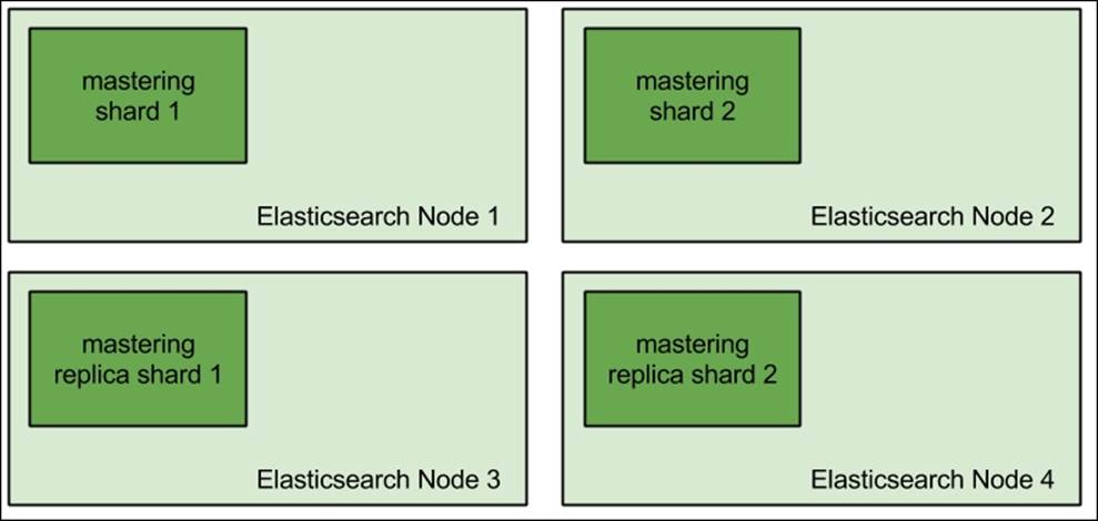
The Elasticsearch replication mechanism not only gives us the ability to handle higher query throughput, but also gives us redundancy and high availability. Imagine an Elasticsearch cluster hosting a single index called mastering that is built of 2 shards and 0 replicas. Such a cluster could look as follows:
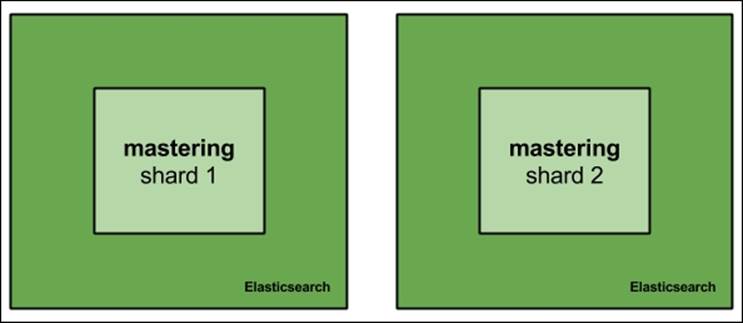
Now, what would happen when one of the nodes fails? The simplest answer is that we lose about 50 percent of the data, and if the failure is fatal, we lose that data forever. Even when having backups, we would need to spin up another node and restore the backup; this takes time. If your business relies on Elasticsearch, downtime means money loss.
Now let's look at the same cluster but with one replica:
Now, losing a single Elasticsearch node means that we still have the whole data available and we can work on restoring the full cluster structure without downtime. What's more, with such deployment, we can live with two nodes failing at the same time in some cases, for example, Node 1 and Node 3 or Node 2 and Node 4. In both the mentioned cases, we would still be able to access all the data. Of course, this will lower performance because of less nodes in the cluster, but this is still better than not handling queries at all.
Because of this, when designing your architecture and deciding on the number of nodes, how many nodes indices will have, and the number of shards for each of them, you should take into consideration how many nodes' failure you want to live with. Of course, you can't forget about the performance part of the equation, but redundancy and high availability should be one of the factors of the scaling equation.
Cost and performance flexibility
The default distributed nature of Elasticsearch and its ability to scale horizontally allow us to be flexible when it comes to performance and costs that we have when running our environment. First of all, high-end servers with highly performant disks, numerous CPU cores, and a lot of RAM are expensive. In addition to this, cloud computing is getting more and more popular and it not only allows us to run our deployment on rented machines, but it also allows us to scale on demand. We just need to add more machines, which is a few clicks away or can even be automated with some degree of work.
Getting this all together, we can say that having a horizontally scalable solution, such as Elasticsearch, allows us to bring down the costs of running our clusters and solutions. What's more, we can easily sacrifice performance if costs are the most crucial factor in our business plan. Of course, we can also go the other way. If we can afford large clusters, we can push Elasticsearch to hundreds of terabytes of data stored in the indices and still get decent performance (of course, with proper hardware and property distributed).
Continuous upgrades
High availability, cost, performance flexibility, and virtually endless growth are not the only things worth saying when discussing the scalability side of Elasticsearch. At some point in time, you will want to have your Elasticsearch cluster to be upgraded to a new version. It can be because of bug fixes, performance improvements, new features, or anything that you can think of. The thing is that when having a single instance of each shard, an upgrade without replicas means the unavailability of Elasticsearch (or at least its parts), and that may mean downtime of the applications that use Elasticsearch. This is another point why horizontal scaling is so important; you can perform upgrades, at least to the point where software such as Elasticsearch is supported. For example, you could take Elasticsearch 1.0 and upgrade it to Elasticsearch 1.4 with only rolling restarts, thus having all the data still available for searching and indexing happening at the same time.
Multiple Elasticsearch instances on a single physical machine
Although we previously said that you shouldn't go for the most powerful machines for different reasons (such as RAM consumption after going above 31 GB JVM heap), we sometimes don't have much choice. This is out of the scope of the book, but because we are talking about scaling, we thought it may be a good thing to mention what can be done in such cases.
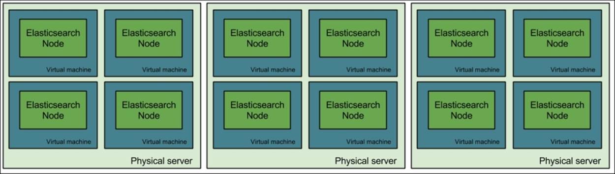
In cases such as the ones we are discussing, when we have high-end hardware with a lot of RAM memory, a lot of high speed disk, numerous CPU cores, among others, we should think about diving the physical server into multiple virtual machines and running a single Elasticsearch server on each of the virtual machines.
Note
There is also a possibility of running multiple Elasticsearch servers on a single physical machine without running multiple virtual machines. Which road to take—virtual machines or multiple instances—is really your choice; however, we like to keep things separate and, because of that, we are usually going to divide any large server into multiple virtual machines. When dividing a large server into multiple smaller virtual machines, remember that the I/O subsystem will be shared across these smaller virtual machines. Because of this, it may be good to wisely divide the disks between virtual machines.
To illustrate such a deployment, please look at the following provided figure. It shows how you could run Elasticsearch on three large servers, each divided into four separate virtual machines. Each virtual machine would be responsible for running a single instance of Elasticsearch.
Preventing the shard and its replicas from being on the same node
There is one additional thing worth mentioning. When having multiple physical servers divided into virtual machines, it is crucial to ensure that the shard and its replica won't end up on the same physical machine. This would be tragic if a server crashes or is restarted. We can tell Elasticsearch to separate shards and replicas using cluster allocation awareness. In our preceding case, we have three physical servers; let's call them server1, server2, and server3.
Now for each Elasticsearch on a physical server, we define the node.server_name property and we set it to the identifier of the server. So, for the example of all Elasticsearch nodes on the first physical server, we would set the following property in theelasticsearch.yml configuration file:
node.server_name: server1
In addition to this, each Elasticsearch node (no matter on which physical server) needs to have the following property added to the elasticsearch.yml configuration file:
cluster.routing.allocation.awareness.attributes: server_name
It tells Elasticsearch not to put the primary shard and its replicas on the nodes with the same value in the node.server_name property. This is enough for us, and Elasticsearch will take care of the rest.
Designated nodes' roles for larger clusters
There is one more thing that we wanted to tell you; actually, we already mentioned that both in the book you are holding in your hands and in Elasticsearch Server Second Edition, Packt Publishing. To have a fully fault-tolerant and highly available cluster, we should divide the nodes and give each node a designated role. The roles we can assign to each Elasticsearch node are as follows:
· The master eligible node
· The data node
· The query aggregator node
By default, each Elasticsearch node is master eligible (it can serve as a master node), can hold data, and can work as a query aggregator node, which means that it can send partial queries to other nodes, gather and merge the results, and respond to the client sending the query. You may wonder why this is needed. Let's give you a simple example: if the master node is under a lot of stress, it may not be able to handle the cluster state-related command fast enough and the cluster can become unstable. This is only a single, simple example, and you can think of numerous others.
Because of this, most Elasticsearch clusters that are larger than a few nodes usually look like the one presented in the following figure:
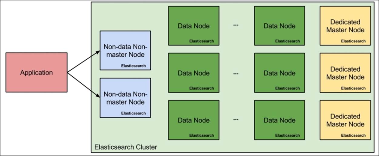
As you can see, our hypothetical cluster contains two aggregator nodes (because we know that there will not be too many queries, but we want redundancy), a dozen of data nodes because the amount of data will be large, and at least three master eligible nodes that shouldn't be doing anything else. Why three master nodes when Elasticsearch will only use a single one at any given time? Again, this is because of redundancy and to be able to prevent split brain situations by setting the discovery.zen.minimum_master_nodes to2, which would allow us to easily handle the failure of a single master eligible node in the cluster.
Let's now give you snippets of the configuration for each type of node in our cluster. We already talked about this in the Discovery and recovery modules section in Chapter 7, Elasticsearch Administration, but we would like to mention it once again.
Query aggregator nodes
The query aggregator nodes' configuration is quite simple. To configure them, we just need to tell Elasticsearch that we don't want these nodes to be master eligible and hold data. This corresponds to the following configuration in the elasticsearch.yml file:
node.master: false
node.data: false
Data nodes
Data nodes are also very simple to configure; we just need to say that they should not be master eligible. However, we are not big fans of default configurations (because they tend to change) and, thus, our Elasticsearch data nodes' configuration looks as follows:
node.master: false
node.data: true
Master eligible nodes
We've left the master eligible nodes for the end of the general scaling section. Of course, such Elasticsearch nodes shouldn't be allowed to hold data, but in addition to that, it is good practice to disable the HTTP protocol on such nodes. This is done in order to avoid accidentally querying these nodes. Master eligible nodes can be smaller in resources compared to data and query aggregator nodes, and because of that, we should ensure that they are only used for master-related purposes. So, our configuration for master eligible nodes looks more or less as follows:
node.master: true
node.data: false
http.enabled: false
Using Elasticsearch for high load scenarios
Now that we know the theory (and some examples of Elasticsearch scaling), we are ready to discuss the different aspects of Elasticsearch preparation for high load. We decided to split this part of the chapter into three sections: one dedicated to preparing Elasticsearch for a high indexing load, one dedicated for the preparation of Elasticsearch for a high query load, and one that can be taken into consideration in both cases. This should give you an idea of what to think about when preparing your cluster for your use case.
Please consider that performance testing should be done after preparing the cluster for production use. Don't just take the values from the book and go for them; try them with your data and your queries and try altering them, and see the differences. Remember that giving general advices that works for everyone is not possible, so treat the next two sections as general advices instead of ready for use recipes.
General Elasticsearch-tuning advices
In this section, we will look at the general advices related to tuning Elasticsearch. They are not connected to indexing performance only or querying performance only but to both of them.
Choosing the right store
One of the crucial aspects of this is that we should choose the right store implementation. This is mostly important when running an Elasticsearch version older than 1.3.0. In general, if you are running a 64-bit operating system, you should again go for mmapfs. If you are not running a 64-bit operating system, choose the niofs store for Unix-based systems and simplefs for Windows-based ones. If you can allow yourself to have a volatile store, but a very fast one, you can look at the memory store: it will give you the best index access performance but requires enough memory to handle not only all the index files, but also to handle indexing and querying.
With the release of Elasticsearch 1.3.0, we've got a new store type called default, which is the new default store type. As Elasticsearch developers said, it is a hybrid store type. It uses memory-mapped files to read term dictionaries and doc values, while the rest of the files are accessed using the NIOFSDirectory implementation. In most cases, when using Elasticsearch 1.3.0 or higher, the default store type should be used.
The index refresh rate
The second thing we should pay attention to is the index refresh rate. We know that the refresh rate specifies how fast documents will be visible for search operations. The equation is quite simple: the faster the refresh rate, the slower the queries will be and the lower the indexing throughput. If we can allow ourselves to have a slower refresh rate, such as 10s or 30s, it may be a good thing to set it. This puts less pressure on Elasticsearch, as the internal objects will have to be reopened at a slower pace and, thus, more resources will be available both for indexing and querying. Remember that, by default, the refresh rate is set to 1s, which basically means that the index searcher object is reopened every second.
To give you a bit of an insight into what performance gains we are talking about, we did some performance tests, including Elasticsearch and a different refresh rate. With a refresh rate of 1s, we were able to index about 1.000 documents per second using a single Elasticsearch node. Increasing the refresh rate to 5s gave us an increase in the indexing throughput of more than 25 percent, and we were able to index about 1280 documents per second. Setting the refresh rate to 25s gave us about 70 percent of throughput more compared to a 1s refresh rate, which was about 1700 documents per second on the same infrastructure. It is also worth remembering that increasing the time indefinitely doesn't make much sense, because after a certain point (depending on your data load and the amount of data you have), the increase in performance is negligible.
Thread pools tuning
This is one of the things that is very dependent on your deployment. By default, Elasticsearch comes with a very good default when it comes to all thread pools' configuration. However, there are times when these defaults are not enough. You should remember that tuning the default thread pools' configuration should be done only when you really see that your nodes are filling up the queues and they still have processing power left that could be designated to the processing of the waiting operations.
For example, if you did your performance tests and you see your Elasticsearch instances not being saturated 100 percent, but on the other hand, you've experienced rejected execution errors, then this is a point where you should start adjusting the thread pools. You can either increase the amount of threads that are allowed to be executed at the same time, or you can increase the queue. Of course, you should also remember that increasing the number of concurrently running threads to very high numbers will lead to many CPU context switches (http://en.wikipedia.org/wiki/Context_switch), which will result in a drop in performance. Of course, having massive queues is also not a good idea; it is usually better to fail fast rather than overwhelm Elasticsearch with several thousands of requests waiting in the queue. However, this all depends on your particular deployment and use case. We would really like to give you a precise number, but in this case, giving general advice is rarely possible.
Adjusting the merge process
Lucene segments' merging adjustments is another thing that is highly dependent on your use case and several factors related to it, such as how much data you add, how often you do that, and so on. There are two things to remember when it comes to Lucene segments and merging. Queries run against an index with multiple segments are slower than the ones with a smaller number of segments. Performance tests show that queries run against an index built of several segments are about 10 to 15 percent slower than the ones run against an index built of only a single segment. On the other hand, though, merging is not free and the fewer segments we want to have in our index, the more aggressive a merge policy should be configured.
Generally, if you want your queries to be faster, aim for fewer segments for your indices. For example, for log_byte_size or log_doc merge policies, setting the index.merge.policy.merge_factor property to a value lower than the default of 10 will result in less segments, lower RAM consumption, faster queries, and slower indexing. Setting the index.merge.policy.merge_factor property to a value higher than 10 will result in more segments building the index, higher RAM consumption, slower queries, and faster indexing.
There is one more thing: throttling. By default, Elasticsearch will throttle merging to 20mb/s. Elasticsearch uses throttling so that your merging process doesn't affect searching too much. What's more, if merging is not fast enough, Elasticsearch will throttle the indexing to be single threaded so that the merging could actually finish and not have an extensive number of segments. However, if you are running SSD drives, the default 20mb/s throttling is probably too much and you can set it to 5 to 10 times more (at least). To adjust throttling, we need to set the indices.store.throttle.max_bytes_per_sec property in elasticsearch.yml (or using the Cluster Settings API) to the desired value, such as 200mb/s.
In general, if you want indexing to be faster, go for more segments for indices. If you want your queries to be faster, your I/O can handle more work because of merging, and you can live with Elasticsearch consuming a bit more RAM memory, go for more aggressive merge policy settings. If you want Elasticsearch to index more documents, go for a less aggressive merge policy, but remember that this will affect your queries' performance. If you want both of these things, you need to find a golden spot between them so that the merging is not too often but also doesn't result in an extensive number of segments.
Data distribution
As we know, each index in the Elasticsearch world can be divided into multiple shards, and each shard can have multiple replicas. In cases where you have multiple Elasticsearch nodes and indices divided into shards, proper data distribution may be crucial to even the load the cluster and not have some nodes doing more work than the other ones.
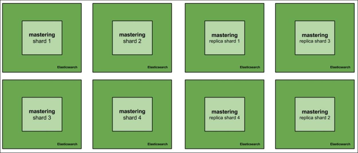
Let's take the following example—imagine that we have a cluster that is built of four nodes, and it has a single index built of three shards and one replica allocated. Such deployment could look as follows:
As you can see, the first two nodes have two physical shards allocated to them, while the last two nodes have one shard each. So the actual data allocation is not even. When sending the queries and indexing data, we will have the first two nodes do more work than the other two; this is what we want to avoid. We could make the mastering index have two shards and one replica so that it would look like this:
Or, we could have the mastering index divided into four shards and have one replica.
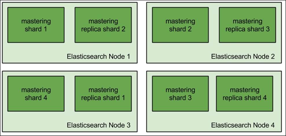
In both cases, we will end up with an even distribution of shards and replicas, with Elasticsearch doing a similar amount of work on all the nodes. Of course, with more indices (such as having daily indices), it may be trickier to get the data evenly distributed, and it may not be possible to have evenly distributed shards, but we should try to get to such a point.
One more thing to remember when it comes to data distribution, shards, and replicas is that when designing your index architecture, you should remember what you want to achieve. If you are going for a very high indexing use case, you may want to spread the index into multiple shards to lower the pressure that is put on the CPU and the I/O subsystem of the server. This is also true in order to run expensive queries, because with more shards, you can lower the load on a single server. However, with queries, there is one more thing: if your nodes can't keep up with the load caused by queries, you can add more Elasticsearch nodes and increase the number of replicas so that physical copies of the primary shards are placed on these nodes. This will make the indexing a bit slower but will give you the capacity to handle more queries at the same time.
Advices for high query rate scenarios
One of the great features of Elasticsearch is its ability to search and analyze the data that was indexed. However, sometimes, the user is needed to adjust Elasticsearch, and our queries to not only get the results of the query, but also get them fast (or in a reasonable amount of time). In this section, we will not only look at the possibilities but also prepare Elasticsearch for high query throughput use cases. We will also look at general performance tips when it comes to querying.
Filter caches and shard query caches
The first cache that can help with query performance is the filter cache (if our queries use filters, and if not, they should probably use filters). We talked about filters in the Handling filters and why it matters section in Chapter 2, Power User Query DSL. What we didn't talk about is the cache that is responsible for storing results of the filters: the filter cache. By default, Elasticsearch uses the filter cache implementation that is shared among all the indices on a single node, and we can control its size using theindices.cache.filter.size property. It defaults to 10 percent by default and specifies the total amount of memory that can be used by the filter cache on a given node. In general, if your queries are already using filters, you should monitor the size of the cache and evictions. If you see that you have many evictions, then you probably have a cache that's too small, and you should consider having a larger one. Having a cache that's too small may impact the query performance in a bad way.
The second cache that has been introduced in Elasticsearch is the shard query cache. It was added to Elasticsearch in Version 1.4.0, and its purpose is to cache aggregations, suggester results, and the number of hits (it will not cache the returned documents and, thus, it only works with search_type=count). When your queries are using aggregations or suggestions, it may be a good idea to enable this cache (it is disabled by default) so that Elasticsearch can reuse the data stored there. The best thing about the cache is that it promises the same near real-time search as search that is not cached.
To enable the shard query cache, we need to set the index.cache.query.enable property to true. For example, to enable the cache for our mastering index, we could issue the following command:
curl -XPUT 'localhost:9200/mastering/_settings' -d '{
"index.cache.query.enable": true
}'
Please remember that using the shard query cache doesn't make sense if we don't use aggregations or suggesters.
One more thing to remember is that, by default, the shard query cache is allowed to take no more than 1 percent of the JVM heap given to the Elasticsearch node. To change the default value, we can use the indices.cache.query.size property. By using theindices.cache.query.expire property, we can specify the expiration date of the cache, but it is not needed, and in most cases, results stored in the cache are invalidated with every index refresh operation.
Think about the queries
This is the most general advice we can actually give: you should always think about optimal query structure, filter usage, and so on. We talked about it extensively in the Handling filters and why it matters section in Chapter 2, Power User Query DSL, but we would like to mention that once again, because we think it is very important. For example, let's look at the following query:
{
"query" : {
"bool" : {
"must" : [
{
"query_string" : {
"query" : "name:mastering AND department:it AND category:book"
}
},
{
"term" : {
"tag" : "popular"
}
},
{
"term" : {
"tag" : "2014"
}
}
]
}
}
}
It returns the book name that matches a few conditions. However, there are a few things we can improve in the preceding query. For example, we could move a few things to filtering so that the next time we use some parts of the query, we save CPU cycles and reuse the information stored in the cache. For example, this is what the optimized query could look like:
{
"query" : {
"filtered" : {
"query" : {
"match" : {
"name" : "mastering"
}
},
"filter" : {
"bool" : {
"must" : [
{
"term" : {
"department" : "it"
}
},
{
"term" : {
"category" : "book"
}
},
{
"terms" : {
"tag" : [ "popular", "2014" ]
}
}
]
}
}
}
}
}
As you can see, there are a few things that we did. First of all, we used the filtered query to introduce filters and we moved most of the static, non-analyzed fields to filters. This allows us to easily reuse the filters in the next queries that we execute. Because of such query restructuring, we were able to simplify the main query, so we changed query_string_query to the match query, because it is enough for our use case. This is exactly what you should be doing when optimizing your queries or designing them—have optimization and performance in mind and try to keep them as optimal as they can be. This will result in faster query execution, lower resource consumption, and better health of the whole Elasticsearch cluster.
However, performance is not the only difference when it comes to the outcome of queries. As you know, filters don't affect the score of the documents returned and are not taken into consideration when calculating the score. Because of this, if you compare the scores returned by the preceding queries for the same documents, you would notice that they are different. This is worth remembering.
Using routing
If your data allows routing, you should consider using it. The data with the same routing value will always end up in the same shard. Because of this, we can save ourselves the need to query all the shards when asking for certain data. For example, if we store the data of our clients, we may use a client identifier as the routing value. This will allow us to store the data of a single client inside a single shard. This means that during querying, Elasticsearch needs to fetch data from only a single shard, as shown in the following figure:
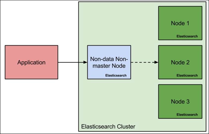
If we assume that the data lives in a shard allocated to Node 2, we can see that Elasticsearch only needed to run the query against that one particular node to get all the data for the client. If we don't use routing, the simplified query execution could look as follows:

In the case of nonrouting, Elasticsearch first needs to query all the index shards. If your index contains dozen of shards, the performance improvement will be significant as long as a single Elasticsearch instance can handle the shard size.
Note
Please remember that not every use case is eligible to use routing. To be able to use it, your data needs to be virtually divided so that it is spread across the shards. For example, it usually doesn't make sense to have dozens of very small shards and one massive one, because for the massive one, performance may not be decent.
Parallelize your queries
One thing that is usually forgotten is the need to parallelize queries. Imagine that you have a dozen nodes in your cluster, but your index is built of a single shard. If the index is large, your queries will perform worse than you would expect. Of course, you can increase the number of replicas, but that won't help; a single query will still go to a single shard in that index, because replicas are not more than the copies of the primary shard, and they contain the same data (or at least they should).
One thing that will actually help is dividing your index into multiple shards—the number of shards depends on the hardware and deployment. In general, it is advised to have the data evenly divided so that nodes are equally loaded. For example, if you have four Elasticsearch nodes and two indices, you may want to have four shards for each index, just like what is shown in the following figure:
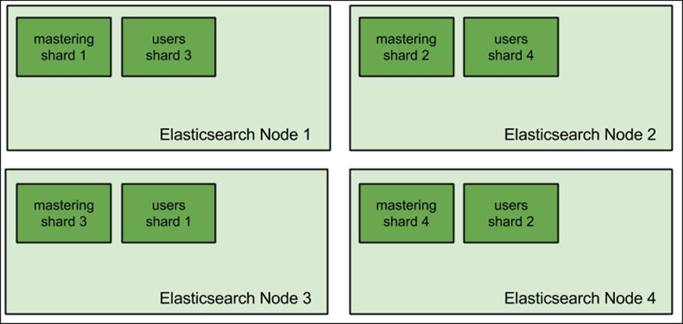
Field data cache and breaking the circuit
By default, the field data cache in Elasticsearch is unbounded. This can be very dangerous, especially when you are using faceting and sorting on many fields. If these fields are high cardinality ones, then you can run into even more trouble. By trouble, we mean running out of memory.
We have two different factors we can tune to be sure that we won't run into out-of-memory errors. First of all, we can limit the size of the field data cache. The second thing is the circuit breaker, which we can easily configure to just throw an exception instead of loading too much data. Combining these two things will ensure that we don't run into memory issues.
However, we should also remember that Elasticsearch will evict data from the field data cache if its size is not enough to handle faceting request or sorting. This will affect the query performance, because loading field data information is not very efficient. However, we think that it is better to have our queries slower rather than having our cluster blown up because of out-of-memory errors.
Finally, if your queries are using field data cache extensively (such as aggregations or sorting) and you are running into memory-related issues (such as OutOfMemory exceptions or GC pauses), consider using doc values that we already talked about. Doc values should give you performance that's similar to field data cache, and support for doc values is getting better and better with each Elasticsearch release (improvements to doc values are made in Lucene itself).
Keeping size and shard_size under control
When dealing with queries that use aggregations, for some of them, we have the possibility of using two properties: size and shard_size. The size parameter defines how many buckets should be returned by the final aggregation results; the node that aggregates the final results will get the top buckets from each shard that returns the result and will only return the top size of them to the client. The shard_size parameter tells Elasticsearch about the same but on the shard level. Increasing the value of the shard_size parameter will lead to more accurate aggregations (such as in the case of significant terms' aggregation) at the cost of network traffic and memory usage. Lowering this parameter will cause aggregation results to be less precise, but we will benefit from lower memory consumption and lower network traffic. If we see that the memory usage is too large, we can lower the size and shard_size properties of problematic queries and see whether the quality of the results is still acceptable.
High indexing throughput scenarios and Elasticsearch
In this section, we will discuss some optimizations that will allow us to concentrate on the indexing throughput and speed. Some use cases are highly dependent on the amount of data you can push to Elasticsearch every second, and the next few topics should cover some information regarding indexing.
Bulk indexing
This is very obvious advice, but you would be surprised by how many Elasticsearch users forget about indexing data in bulk instead of sending the documents one by one. The thing to remember, though, is to not overload Elasticsearch with too many bulk requests. Remember about the bulk thread pool and its size (equal to the number of CPU cores in the system by default with a queue of 50 requests), and try to adjust your indexers so that they don't to go beyond it. Or, you will first start to queue their requests and if Elasticsearch is not able to process them, you will quickly start seeing rejected execution exceptions, and your data won't be indexed. On the other hand, remember that your bulk requests can't be too large, or Elasticsearch will need a lot of memory to process them.
Just as an example, I would like to show you two types of indexing happening. In the first figure, we have indexing throughput when running the indexation one document by one. In the second figure, we do the same, but instead of indexing documents one by one, we index them in batches of 10 documents.
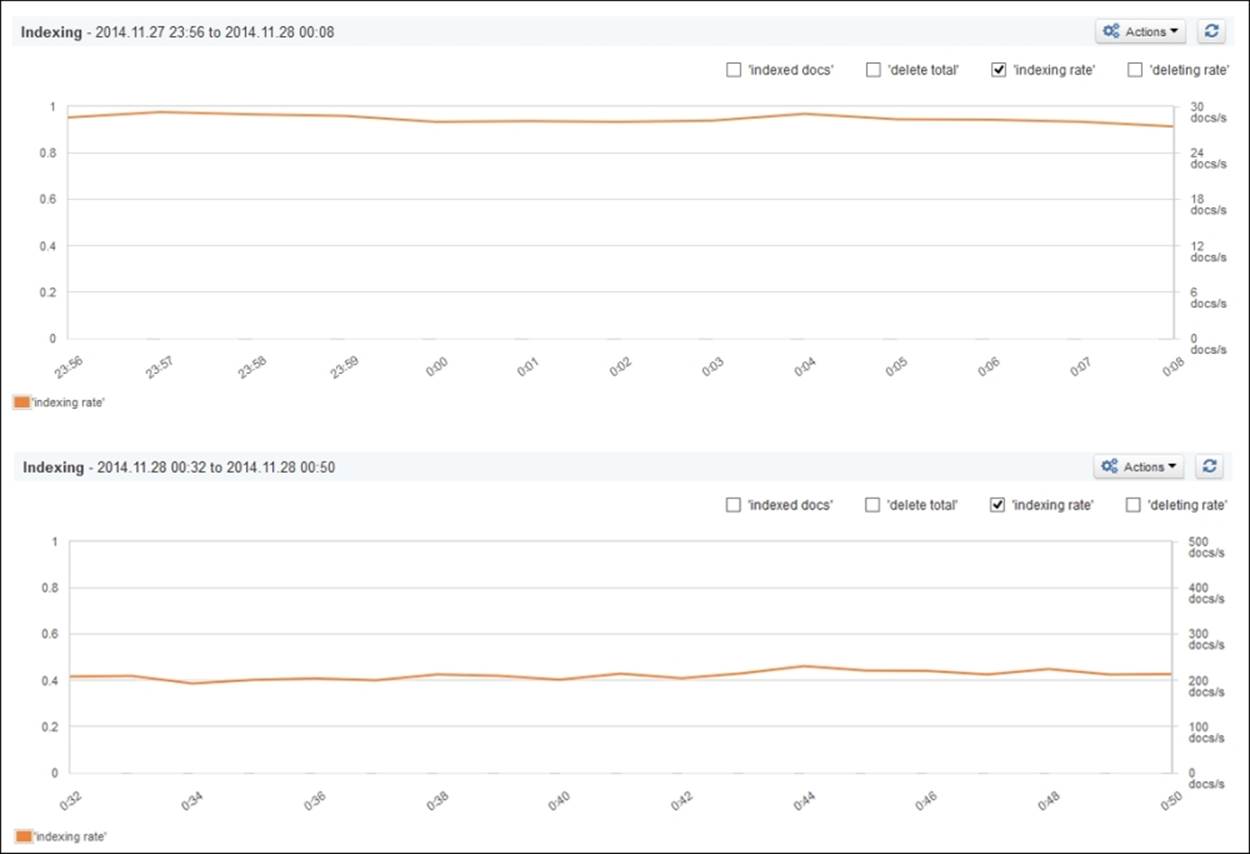
As you can see, when indexing documents one by one, we were able to index about 30 documents per second and it was stable. The situation changed with bulk indexing and batches of 10 documents. We were able to index slightly more than 200 documents per second, so the difference can be clearly seen.
Of course, this is a very basic comparison of indexing speed, and in order to show you the real difference, we should use dozens of threads and push Elasticsearch to its limits. However, the preceding comparison should give you a basic view of the indexing throughput gains when using bulk indexing.
Doc values versus indexing speed
When talking about indexing speed, we have to talk about doc values. As we already said a few times in the book, doc values allows us to fight gigantic JVM heap requirements when Elasticsearch needs to uninvert fields for functionalities such as sorting, aggregations, or faceting. However, writing doc values requires some additional work during the indexation. If we are all about the highest indexing speed and the most indexing throughput, you should consider not going for doc values. On the other hand, if you have a lot of data—and you probably have when you are indexing fast—using doc values may be the only way that will allow using aggregations or sorting on field values without running into memory-related problems.
Keep your document fields under control
The amount of data you index makes the difference, which is understandable. However, this is not the only factor; the size of the documents and their analysis matters as well. With larger documents, you can expect not only your index to grow, but also make the indexation slightly slower. This is why you may sometimes want to look at all the fields you are indexing and storing. Keep your stored fields to a minimum or don't use them at all; the only stored field you need in most cases is the _source field.
There is one more thing—apart from the _source field, Elasticsearch indexes the _all field by default. Let's remind you: the _all field is used by Elasticsearch to gather data from all the other textual fields. In some cases, this field is not used at all and because of that, it is nice to turn it off. Turning it off is simple and the only thing to do is add the following entry to the type mappings:
"_all" : {"enabled" : false}
We can do this during the index creation, for example, like this:
curl -XPOST 'localhost:9200/disabling_all' -d '{
"mappings" : {
"test_type" : {
"_all" : { "enabled" : false },
"properties" : {
"name" : { "type" : "string" },
"tag" : { "type" : "string", "index" : "not_analyzed" }
}
}
}
}'
The indexing should be slightly faster depending on the size of your documents and the number of textual fields in it.
There is an additional thing, which is good practice when disabling the _all field: setting a new default search field. We can do this by setting the index.query.default_field property. For example, in our case, we can set it in the elasticsearch.yml file and set it to thename field from our preceding mappings:
index.query.default_field: name
The index architecture and replication
When designing the index architecture, one of the things you need to think about is the number of shards and replicas that the index is built of. During that time, we also need to we think about data distribution among Elasticsearch nodes, optimal performance, high availability, reliability, and so on. First of all, distributing primary shards of the index across all nodes we have will parallelize indexing operations and will make them faster.
The second thing is data replication. What we have to remember is that too many replicas will cause the indexation speed to drop. This is because of several reasons. First of all, you need to transfer the data between primary shards and replicas. The second thing is that, usually, replicas and primary shards may live on the same nodes (not primary shards and its replicas, of course, but replicas of other primaries). For example, take a look at what is shown in the following figure:
Because of this, Elasticsearch will need the data for both primary shards and replicas and, thus, it will use the disk. Depending on the cluster setup, the indexing throughput may drop in such cases (depends on the disks, number of documents indexed at the same time, and so on).
Tuning write-ahead log
We already talked about transaction logs in the Data flushing, index refresh and transaction log handling section of Chapter 6, Low-level Index Control. Elasticsearch has an internal module called translog (http://www.elasticsearch.org/guide/en/elasticsearch/reference/current/index-modules-translog.html). It is a per-shard structure that serves the purpose of write-ahead logging (http://en.wikipedia.org/wiki/Write-ahead_logging). Basically, it allows Elasticsearch to expose the newest updates for GET operations, ensure data durability, and optimize writing to Lucene indices.
By default, Elasticsearch keeps a maximum of 5000 operations in the transaction log with a maximum size of 200 MB. However, if we can pay the price of data not being available for search operations for longer periods of time but we want more indexing throughput, we can increase these defaults. By specifying the index.translog.flush_threshold_ops and index.translog.flush_threshold_size properties (both are set per index and can be updated in real time using the Elasticsearch API), we can set the maximum number of operations allowed to be stored in the transaction log and its maximum size. We've seen deployments having this property values set to 10 times the default values.
One thing to remember is that in case of failure, shard initialization will be slower—of course on the ones that had large transaction logs. This is because Elasticsearch needs to process all the information from the transaction log before the shard is ready for use.
Think about storage
One of the crucial things when it comes to high indexing use cases is the storage type and its configuration. If your organization can afford SSD disks (solid state drives), go for them. They are superior in terms of speed compared to the traditional spinning disks, but of course, that comes at the cost of price. If you can't afford SSD drives, configure your spinning disks to work in RAID 0 (http://en.wikipedia.org/wiki/RAID) or point Elasticsearch to use multiple data paths.
What's more, don't use shared or remote filesystems for Elasticsearch indices; use local storage instead. Remote and shared filesystems are usually slower compared to local disk drives and will cause Elasticsearch to wait for read and write, and thus result in a general slowdown.
RAM buffer for indexing
Remember that the more the available RAM for the indexing buffer (the indices.memory.index_buffer_size property), the more documents Elasticsearch can hold in the memory, but of course, we don't want to occupy 100 percent of the available memory only to Elasticsearch. By default, this is set to 10 percent, but if you really need a high indexing rate, you can increase it. It is advisable to have approximately 512 MB of RAM for each active shard that takes part in the indexing process, but remember that theindices.memory.index_buffer_size property is per node and not per shard. So, if you have 20 GB of heap given to the Elasticsearch node and 10 shards active on the node, Elasticsearch will give each shard about 200 MB of RAM for indexing buffering (10 percent of 20 GB / 10 shards) by default.
Summary
In this chapter, we were focused on the performance and scaling of Elasticsearch. We looked at how doc values can help us with improving the query performance, how garbage collector works, and what to look at when changing its configuration. We benchmarked our queries and we saw what the Hot Threads API is. Finally, we discussed how to scale Elasticsearch and how to prepare it for high querying and indexing use cases.
In the next chapter, we will write some code. We will create the Apache Maven project used to write Elasticsearch plugins. We will write a custom REST action to extend the Elasticsearch functionality. In addition to this, we will learn what needs to be done in order to introduce new analysis plugins for Elasticsearch, and we will create such plugins.
All materials on the site are licensed Creative Commons Attribution-Sharealike 3.0 Unported CC BY-SA 3.0 & GNU Free Documentation License (GFDL)
If you are the copyright holder of any material contained on our site and intend to remove it, please contact our site administrator for approval.
© 2016-2026 All site design rights belong to S.Y.A.