Elasticsearch Server, Second Edition (2014)
Chapter 2. Indexing Your Data
In the previous chapter, we learned the basics about full text search and Elasticsearch. We also saw what Apache Lucene is. In addition to that, we saw how to install Elasticsearch, what the standard directory layout is, and what to pay attention to. We created an index, and we indexed and updated our data. Finally, we used the simple URI query to get data from Elasticsearch. By the end of this chapter, you will learn the following topics:
· Elasticsearch indexing
· Configuring your index structure mappings and knowing what field types we are allowed to use
· Using batch indexing to speed up the indexing process
· Extending your index structure with additional internal information
· Understanding what segment merging is, how to configure it, and what throttling is
· Understanding how routing works and how we can configure it to our needs
Elasticsearch indexing
We have our Elasticsearch cluster up and running, and we also know how to use the Elasticsearch REST API to index our data, delete it, and retrieve it. We also know how to use search to get our documents. If you are used to SQL databases, you might know that before you can start putting the data there, you need to create a structure, which will describe what your data looks like. Although Elasticsearch is a schema-less search engine and can figure out the data structure on the fly, we think that controlling the structure and thus defining it ourselves is a better way. In the following few pages, you'll see how to create new indices (and how to delete them). Before we look closer at the available API methods, let's see what the indexing process looks like.
Shards and replicas
As you recollect from the previous chapter, the Elasticsearch index is built of one or more shards and each of them contains part of your document set. Each of these shards can also have replicas, which are exact copies of the shard. During index creation, we can specify how many shards and replicas should be created. We can also omit this information and use the default values either defined in the global configuration file (elasticsearch.yml) or implemented in Elasticsearch internals. If we rely on Elasticsearch defaults, our index will end up with five shards and one replica. What does that mean? To put it simply, we will end up with having 10 Lucene indices distributed among the cluster.
Note
Are you wondering how we did the calculation and got 10 Lucene indices from five shards and one replica? The term "replica" is somewhat misleading. It means that every shard has its copy, so it means there are five shards and five copies.
Having a shard and its replica, in general, means that when we index a document, we will modify them both. That's because to have an exact copy of a shard, Elasticsearch needs to inform all the replicas about the change in shard contents. In the case of fetching a document, we can use either the shard or its copy. In a system with many physical nodes, we will be able to place the shards and their copies on different nodes and thus use more processing power (such as disk I/O or CPU). To sum up, the conclusions are as follows:
· More shards allow us to spread indices to more servers, which means we can handle more documents without losing performance.
· More shards means that fewer resources are required to fetch a particular document because fewer documents are stored in a single shard compared to the documents stored in a deployment with fewer shards.
· More shards means more problems when searching across the index because we have to merge results from more shards and thus the aggregation phase of the query can be more resource intensive.
· Having more replicas results in a fault tolerance cluster, because when the original shard is not available, its copy will take the role of the original shard. Having a single replica, the cluster may lose the shard without data loss. When we have two replicas, we can lose the primary shard and its single replica and still everything will work well.
· The more the replicas, the higher the query throughput will be. That's because the query can use either a shard or any of its copies to execute the query.
Of course, these are not the only relationships between the number of shards and replicas in Elasticsearch. We will talk about most of them later in the book.
So, how many shards and replicas should we have for our indices? That depends. We believe that the defaults are quite good but nothing can replace a good test. Note that the number of replicas is less important because you can adjust it on a live cluster after index creation. You can remove and add them if you want and have the resources to run them. Unfortunately, this is not true when it comes to the number of shards. Once you have your index created, the only way to change the number of shards is to create another index and reindex your data.
Creating indices
When we created our first document in Elasticsearch, we didn't care about index creation at all. We just used the following command:
curl -XPUT http://localhost:9200/blog/article/1 -d '{"title": "New version of Elasticsearch released!", "content": "...", "tags": ["announce", "elasticsearch", "release"] }'
This is fine. If such an index does not exist, Elasticsearch automatically creates the index for us. We can also create the index ourselves by running the following command:
curl -XPUT http://localhost:9200/blog/
We just told Elasticsearch that we want to create the index with the blog name. If everything goes right, you will see the following response from Elasticsearch:
{"acknowledged":true}
When is manual index creation necessary? There are many situations. One of them can be the inclusion of additional settings such as the index structure or the number of shards.
Altering automatic index creation
Sometimes, you can come to the conclusion that automatic index creation is a bad thing. When you have a big system with many processes sending data into Elasticsearch, a simple typo in the index name can destroy hours of script work. You can turn off automatic index creation by adding the following line in the elasticsearch.yml configuration file:
action.auto_create_index: false
Note
Note that action.auto_create_index is more complex than it looks. The value can be set to not only false or true. We can also use index name patterns to specify whether an index with a given name can be created automatically if it doesn't exist. For example, the following definition allows automatic creation of indices with the names beginning with a, but disallows the creation of indices starting with an. The other indices aren't allowed and must be created manually (because of -*).
action.auto_create_index: -an*,+a*,-*
Note that the order of pattern definitions matters. Elasticsearch checks the patterns up to the first pattern that matches, so if you move -an* to the end, it won't be used because of +a*, which will be checked first.
Settings for a newly created index
The manual creation of an index is also necessary when you want to set some configuration options, such as the number of shards and replicas. Let's look at the following example:
curl -XPUT http://localhost:9200/blog/ -d '{"settings" : {
"number_of_shards" : 1,
"number_of_replicas" : 2
}
}'
The preceding command will result in the creation of the blog index with one shard and two replicas, so it makes a total of three physical Lucene indices. Also, there are other values that can be set in this way; we will talk about those later in the book.
So, we already have our new, shiny index. But there is a problem; we forgot to provide the mappings, which are responsible for describing the index structure. What can we do? Since we have no data at all, we'll go for the simplest approach – we will just delete the index. To do that, we will run a command similar to the preceding one, but instead of using the PUT HTTP method, we use DELETE. So the actual command is as follows:
curl –XDELETE http://localhost:9200/posts
And the response will be the same as the one we saw earlier, as follows:
{"acknowledged":true}
Now that we know what an index is, how to create it, and how to delete it, we are ready to create indices with the mappings we have defined. It is a very important part because data indexation will affect the search process and the way in which documents are matched.
Mappings configuration
If you are used to SQL databases, you may know that before you can start inserting the data in the database, you need to create a schema, which will describe what your data looks like. Although Elasticsearch is a schema-less search engine and can figure out the data structure on the fly, we think that controlling the structure and thus defining it ourselves is a better way. In the following few pages, you'll see how to create new indices (and how to delete them) and how to create mappings that suit your needs and match your data structure.
Note
Note that we didn't include all the information about the available types in this chapter and some features of Elasticsearch, such as nested type, parent-child handling, storing geographical points, and search, are described in the following chapters of this book.
Type determining mechanism
Before we start describing how to create mappings manually, we wanted to write about one thing. Elasticsearch can guess the document structure by looking at JSON, which defines the document. In JSON, strings are surrounded by quotation marks, Booleans are defined using specific words, and numbers are just a few digits. This is a simple trick, but it usually works. For example, let's look at the following document:
{
"field1": 10,
"field2": "10"
}
The preceding document has two fields. The field1 field will be determined as a number (to be precise, as long type), but field2 will be determined as a string, because it is surrounded by quotation marks. Of course, this can be the desired behavior, but sometimes the data source may omit the information about the data type and everything may be present as strings. The solution to this is to enable more aggressive text checking in the mapping definition by setting the numeric_detection property to true. For example, we can execute the following command during the creation of the index:
curl -XPUT http://localhost:9200/blog/?pretty -d '{
"mappings" : {
"article": {
"numeric_detection" : true
}
}
}'
Unfortunately, the problem still exists if we want the Boolean type to be guessed. There is no option to force the guessing of Boolean types from the text. In such cases, when a change of source format is impossible, we can only define the field directly in themappings definition.
Another type that causes trouble is a date-based one. Elasticsearch tries to guess dates given as timestamps or strings that match the date format. We can define the list of recognized date formats using the dynamic_date_formats property, which allows us to specifythe formats array. Let's look at the following command for creating the index and type:
curl -XPUT 'http://localhost:9200/blog/' -d '{
"mappings" : {
"article" : {
"dynamic_date_formats" : ["yyyy-MM-dd hh:mm"]
}
}
}'
The preceding command will result in the creation of an index called blog with the single type called article. We've also used the dynamic_date_formats property with a single date format that will result in Elasticsearch using the date core type (please refer to the Core types section in this chapter for more information about field types) for fields matching the defined format. Elasticsearch uses the joda-time library to define date formats, so please visit http://joda-time.sourceforge.net/api-release/org/joda/time/format/DateTimeFormat.html if you are interested in finding out more about them.
Note
Remember that the dynamic_date_format property accepts an array of values. That means that we can handle several date formats simultaneously.
Disabling field type guessing
Let's think about the following case. First we index a number, an integer. Elasticsearch will guess its type and will set the type to integer or long (refer to the Core types section in this chapter for more information about field types). What will happen if we index a document with a floating point number into the same field? Elasticsearch will just remove the decimal part of the number and store the rest. Another reason for turning it off is when we don't want to add new fields to an existing index—the fields that were not known during application development.
To turn off automatic field adding, we can set the dynamic property to false. We can add the dynamic property as the type property. For example, if we would like to turn off automatic field type guessing for the article type in the blog index, our command will look as follows:
curl -XPUT 'http://localhost:9200/blog/' -d '{
"mappings" : {
"article" : {
"dynamic" : "false",
"properties" : {
"id" : { "type" : "string" },
"content" : { "type" : "string" },
"author" : { "type" : "string" }
}
}
}
}'
After creating the blog index using the preceding command, any field that is not mentioned in the properties section (we will discuss this in the next section) will be ignored by Elasticsearch. So any field apart from id, content, and author will just be ignored. Of course, this is only true for the article type in the blog index.
Index structure mapping
The schema mapping (or in short, mappings) is used to define the index structure. As you may recall, each index can have multiple types, but we will concentrate on a single type for now—just for simplicity. Let's assume that we want to create an index called poststhat will hold data for blog posts. It could have the following structure:
· Unique identifier
· Name
· Publication date
· Contents
In Elasticsearch, mappings are sent as JSON objects in a file. So, let's create a mapping file that will match the aforementioned needs—we will call it posts.json. Its content is as follows:
{
"mappings": {
"post": {
"properties": {
"id": {"type":"long", "store":"yes",
"precision_step":"0" },
"name": {"type":"string", "store":"yes",
"index":"analyzed" },
"published": {"type":"date", "store":"yes",
"precision_step":"0" },
"contents": {"type":"string", "store":"no",
"index":"analyzed" }
}
}
}
}
To create our posts index with the preceding file, run the following command (assuming that we stored the mappings in the posts.json file):
curl -XPOST 'http://localhost:9200/posts' -d @posts.json
Note
Note that you can store your mappings and set a file named anyway you want.
And again, if everything goes well, we see the following response:
{"acknowledged":true}
Now we have our index structure and we can index our data. Let's take a break to discuss the contents of the posts.json file.
Type definition
As you can see, the contents of the posts.json file are JSON objects and therefore it starts and ends with curly brackets (if you want to learn more about JSON, please visit http://www.json.org/). All the type definitions inside the mentioned file are nested in themappings object. You can define multiple types inside the mappings JSON object. In our example, we have a single post type. But, for example, if we would also like to include the user type, the file will look as follows:
{
"mappings": {
"post": {
"properties": {
"id": { "type":"long", "store":"yes",
"precision_step":"0" },
"name": { "type":"string", "store":"yes",
"index":"analyzed" },
"published": { "type":"date", "store":"yes",
"precision_step":"0" },
"contents": { "type":"string", "store":"no",
"index":"analyzed" }
}
},
"user": {
"properties": {
"id": { "type":"long", "store":"yes",
"precision_step":"0" },
"name": { "type":"string", "store":"yes",
"index":"analyzed" }
}
}
}
}
Fields
Each type is defined by a set of properties—fields that are nested inside the properties object. So let's concentrate on a single field now; for example, the contents field, whose definition is as follows:
"contents": { "type":"string", "store":"yes", "index":"analyzed" }
It starts with the name of the field, which is contents in the preceding case. After the name of the field, we have an object defining the behavior of the field. The attributes are specific to the types of fields we are using and we will discuss them in the next section. Of course, if you have multiple fields for a single type (which is what we usually have), remember to separate them with a comma.
Core types
Each field type can be specified to a specific core type provided by Elasticsearch. The core types in Elasticsearch are as follows:
· String
· Number
· Date
· Boolean
· Binary
So, now let's discuss each of the core types available in Elasticsearch and the attributes it provides to define their behavior.
Common attributes
Before continuing with all the core type descriptions, we would like to discuss some common attributes that you can use to describe all the types (except for the binary one).
· index_name: This defines the name of the field that will be stored in the index. If this is not defined, the name will be set to the name of the object that the field is defined with.
· index: This can take the values analyzed and no. Also, for string-based fields, it can also be set to not_analyzed. If set to analyzed, the field will be indexed and thus searchable. If set to no, you won't be able to search on such a field. The default value is analyzed. In the case of string-based fields, there is an additional option, not_analyzed. This, when set, will mean that the field will be indexed but not analyzed. So, the field is written in the index as it was sent to Elasticsearch and only a perfect match will be counted during a search. Setting the index property to no will result in the disabling of the include_in_all property of such a field.
· store: This can take the values yes and no and specifies if the original value of the field should be written into the index. The default value is no, which means that you can't return that field in the results (although, if you use the _source field, you can return the value even if it is not stored), but if you have it indexed, you can still search the data on the basis of it.
· boost: The default value of this attribute is 1. Basically, it defines how important the field is inside the document; the higher the boost, the more important the values in the field.
· null_value: This attribute specifies a value that should be written into the index in case that field is not a part of an indexed document. The default behavior will just omit that field.
· copy_to: This attribute specifies a field to which all field values will be copied.
· include_in_all: This attribute specifies if the field should be included in the _all field. By default, if the _all field is used, all the fields will be included in it. The _all field will be described in more detail in the Extending your index structure with additional internal information section.
String
String is the most basic text type, which allows us to store one or more characters inside it. A sample definition of such a field can be as follows:
"contents" : { "type" : "string", "store" : "no", "index" : "analyzed" }
In addition to the common attributes, the following attributes can also be set for string-based fields:
· term_vector: This attribute can take the values no (the default one), yes, with_offsets, with_positions, and with_positions_offsets. It defines whether or not to calculate the Lucene term vectors for that field. If you are using highlighting, you will need to calculate the term vector.
· omit_norms: This attribute can take the value true or false. The default value is false for string fields that are analyzed and true for string fields that are indexed but not analyzed. When this attribute is set to true, it disables the Lucene norms calculation for that field (and thus you can't use index-time boosting), which can save memory for fields used only in filters (and thus not being taken into consideration when calculating the score of the document).
· analyzer: This attribute defines the name of the analyzer used for indexing and searching. It defaults to the globally-defined analyzer name.
· index_analyzer: This attribute defines the name of the analyzer used for indexing.
· search_analyzer: This attribute defines the name of the analyzer used for processing the part of the query string that is sent to a particular field.
· norms.enabled: This attribute specifies whether the norms should be loaded for a field. By default, it is set to true for analyzed fields (which means that the norms will be loaded for such fields) and to false for non-analyzed fields.
· norms.loading: This attribute takes the values eager and lazy. The first value means that the norms for such fields are always loaded. The second value means that the norms will be loaded only when needed.
· position_offset_gap: This attribute defaults to 0 and specifies the gap in the index between instances of the given field with the same name. Setting this to a higher value may be useful if you want position-based queries (like phrase queries) to match only inside a single instance of the field.
· index_options: This attribute defines the indexing options for the postings list—the structure holding the terms (we will talk about this more in The postings format section of this chapter). The possible values are docs (only document numbers are indexed), freqs(document numbers and term frequencies are indexed), positions (document numbers, term frequencies, and their positions are indexed), and offsets (document numbers, term frequencies, their positions, and offsets are indexed). The default value for this property is positions for analyzed fields and docs for fields that are indexed but not analyzed.
· ignore_above: This attribute defines the maximum size of the field in characters. Fields whose size is above the specified value will be ignored by the analyzer.
Number
This is the core type that gathers all numeric field types that are available to be used. The following types are available in Elasticsearch (we specify them by using the type property):
· byte: This type defines a byte value; for example, 1
· short: This type defines a short value; for example, 12
· integer: This type defines a integer value; for example, 134
· long: This type defines a long value; for example, 123456789
· float: This type defines a float value; for example, 12.23
· double: This type defines a double value; for example, 123.45
Note
You can learn more about the mentioned Java types at http://docs.oracle.com/javase/tutorial/java/nutsandbolts/datatypes.html.
A sample definition of a field based on one of the numeric types is as follows:
"price" : { "type" : "float", "store" : "yes", "precision_step" : "4"}
In addition to the common attributes, the following ones can also be set for the numeric fields:
· precision_step: This attribute specifies the number of terms generated for each value in a field. The lower the value, the higher the number of terms generated. For fields with a higher number of terms per value, range queries will be faster at the cost of a slightly larger index. The default value is 4.
· ignore_malformed: This attribute can take the value true or false. The default value is false. It should be set to true in order to omit badly formatted values.
Boolean
The boolean core type is designed for indexing Boolean values (true or false). A sample definition of a field based on the boolean type can be as follows:
"allowed" : { "type" : "boolean", "store": "yes" }
Binary
The binary field is a Base64 representation of the binary data stored in the index. You can use it to store data that is normally written in binary form, such as images. Fields based on this type are by default stored and not indexed, so you can only retrieve them and cannot perform search operations on them. The binary type only supports the index_name property. The sample field definition based on the binary field may look like the following:
"image" : { "type" : "binary" }
Date
The date core type is designed to be used for date indexing. It follows a specific format that can be changed and is stored in UTC by default.
The default date format understood by Elasticsearch is quite universal and allows the specifying of the date and optionally the time, for example, 2012-12-24T12:10:22. A sample definition of a field based on the date type is as follows:
"published" : { "type" : "date", "store" : "yes", "format" : "YYYY-mm-dd" }
A sample document that uses the preceding field is as follows:
{
"name" : "Sample document",
"published" : "2012-12-22"
}
In addition to the common attributes, the following ones can also be set for the fields based on the date type:
· format: This attribute specifies the format of the date. The default value is dateOptionalTime. For a full list of formats, please visit http://www.elasticsearch.org/guide/en/elasticsearch/reference/current/mapping-date-format.html.
· precision_step: This attribute specifies the number of terms generated for each value in that field. The lower the value, the higher the number of terms generated, and thus the faster the range queries (but with a higher index size). The default value is 4.
· ignore_malformed: This attribute can take the value true or false. The default value is false. It should be set to true in order to omit badly formatted values.
Multifields
Sometimes, you would like to have the same field values in two fields; for example, one for searching and one for sorting, or one analyzed with the language analyzer and one only on the basis of whitespace characters. Elasticsearch addresses this need by allowing the addition of the fields object to the field definition. It allows the mapping of several core types into a single field and having them analyzed separately. For example, if we would like to calculate faceting and search on our name field, we can define the following field:
"name": {
"type": "string",
"fields": {
"facet": { "type" : "string", "index": "not_analyzed" }
}
}
The preceding definition will create two fields: we will refer to the first as name and the second as name.facet. Of course, you don't have to specify two separate fields during indexing—a single one named name is enough; Elasticsearch will do the rest, which means copying the value of the field to all the fields from the preceding definition.
The IP address type
The ip field type was added to Elasticsearch to simplify the use of IPv4 addresses in a numeric form. This field type allows us to search data that is indexed as an IP address, sort on this data, and use range queries using IP values.
A sample definition of a field based on one of the numeric types is as follows:
"address" : { "type" : "ip", "store" : "yes" }
In addition to the common attributes, the precision_step attribute can also be set for the numeric fields. This attribute specifies the number of terms generated for each value in a field. The lower the value, the higher the number of terms generated. For fields with a higher number of terms per value, range queries will be faster at the cost of a slightly larger index. The default value is 4.
A sample document that uses the preceding field is as follows:
{
"name" : "Tom PC",
"address" : "192.168.2.123"
}
The token_count type
The token_count field type allows us to store index information about how many words the given field has instead of storing and indexing the text provided to the field. It accepts the same configuration options as the number type, but in addition to that, it allows us to specify the analyzer by using the analyzer property.
A sample definition of a field based on the token_count field type looks as follows:
"address_count" : { "type" : "token_count", "store" : "yes" }
Using analyzers
As we mentioned, for the fields based on the string type, we can specify which analyzer the Elasticsearch should use. As you remember from the Full-text searching section of Chapter 1, Getting Started with the Elasticsearch Cluster, the analyzer is a functionality that is used to analyze data or queries in a way we want. For example, when we divide words on the basis of whitespaces and lowercase characters, we don't have to worry about users sending words in lowercase or uppercase. Elasticsearch allows us to use different analyzers at the time of indexing and different analyzers at the time of querying—we can choose how we want our data to be processed at each stage of the search process. To use one of the analyzers, we just need to specify its name to the correct property of the field and that's all.
Out-of-the-box analyzers
Elasticsearch allows us to use one of the many analyzers defined by default. The following analyzers are available out of the box:
· standard: This is a standard analyzer that is convenient for most European languages (please refer to http://www.elasticsearch.org/guide/en/elasticsearch/reference/current/analysis-standard-analyzer.html for the full list of parameters).
· simple: This is an analyzer that splits the provided value depending on non-letter characters and converts them to lowercase.
· whitespace: This is an analyzer that splits the provided value on the basis of whitespace characters
· stop: This is similar to a simple analyzer, but in addition to the functionality of the simple analyzer, it filters the data on the basis of the provided set of stop words (please refer to http://www.elasticsearch.org/guide/en/elasticsearch/reference/current/analysis-stop-analyzer.html for the full list of parameters).
· keyword: This is a very simple analyzer that just passes the provided value. You'll achieve the same by specifying a particular field as not_analyzed.
· pattern: This is an analyzer that allows flexible text separation by the use of regular expressions (please refer to http://www.elasticsearch.org/guide/en/elasticsearch/reference/current/analysis-pattern-analyzer.html for the full list of parameters).
· language: This is an analyzer that is designed to work with a specific language. The full list of languages supported by this analyzer can be found at http://www.elasticsearch.org/guide/en/elasticsearch/reference/current/analysis-lang-analyzer.html.
· snowball: This is an analyzer that is similar to standard, but additionally provides the stemming algorithm (please refer to http://www.elasticsearch.org/guide/en/elasticsearch/reference/current/analysis-snowball-analyzer.html for the full list of parameters).
Note
Stemming is the process of reducing inflected and derived words to their stem or base form. Such a process allows for the reduction of words, for example, with cars and car. For the mentioned words, stemmer (which is an implementation of the stemming algorithm) will produce a single stem, car. After indexing, documents containing such words will be matched while using any of them. Without stemming, documents with the word "cars" will only be matched by a query containing the same word.
Defining your own analyzers
In addition to the analyzers mentioned previously, Elasticsearch allows us to define new ones without the need to write a single line of Java code. In order to do that, we need to add an additional section to our mappings file; that is, the settings section, which holds useful information required by Elasticsearch during index creation. The following is how we define our custom settings section:
"settings" : {
"index" : {
"analysis": {
"analyzer": {
"en": {
"tokenizer": "standard",
"filter": [
"asciifolding",
"lowercase",
"ourEnglishFilter"
]
}
},
"filter": {
"ourEnglishFilter": {
"type": "kstem"
}
}
}
}
}
We specified that we want a new analyzer named en to be present. Each analyzer is built from a single tokenizer and multiple filters. A complete list of default filters and tokenizers can be found athttp://www.elasticsearch.org/guide/en/elasticsearch/reference/current/analysis.html. Our en analyzer includes the standard tokenizer and three filters: asciifolding and lowercase, which are the ones available by default, and ourEnglishFilter, which is a filter we have defined.
To define a filter, we need to provide its name, its type (the type property), and any number of additional parameters required by that filter type. The full list of filter types available in Elasticsearch can be found athttp://www.elasticsearch.org/guide/en/elasticsearch/reference/current/analysis.html. This list changes constantly, so we'll skip commenting on it.
So, the final mappings file with the analyzer defined will be as follows:
{
"settings" : {
"index" : {
"analysis": {
"analyzer": {
"en": {
"tokenizer": "standard",
"filter": [
"asciifolding",
"lowercase",
"ourEnglishFilter"
]
}
},
"filter": {
"ourEnglishFilter": {
"type": "kstem"
}
}
}
}
},
"mappings" : {
"post" : {
"properties" : {
"id": { "type" : "long", "store" : "yes",
"precision_step" : "0" },
"name": { "type" : "string", "store" : "yes", "index" :
"analyzed", "analyzer": "en" }
}
}
}
}
We can see how our analyzer works by using the Analyze API (http://www.elasticsearch.org/guide/en/elasticsearch/reference/current/indices-analyze.html). For example, let's look at the following command:
curl -XGET 'localhost:9200/posts/_analyze?pretty&field=post.name' -d 'robots cars'
The command asks Elasticsearch to show the content of the analysis of the given phrase (robots cars) with the use of the analyzer defined for the post type and its name field. The response that we will get from Elasticsearch is as follows:
{
"tokens" : [ {
"token" : "robot",
"start_offset" : 0,
"end_offset" : 6,
"type" : "<ALPHANUM>",
"position" : 1
}, {
"token" : "car",
"start_offset" : 7,
"end_offset" : 11,
"type" : "<ALPHANUM>",
"position" : 2
} ]
}
As you can see, the robots cars phrase was divided into two tokens. In addition to that, the robots word was changed to robot and the cars word was changed to car.
Analyzer fields
An analyzer field (_analyzer) allows us to specify a field value that will be used as the analyzer name for the document to which the field belongs. Imagine that you have a software running that detects the language the document is written in and you store that information in the language field in the document. In addition to that, you would like to use that information to choose the right analyzer. To do that, just add the following lines to your mappings file:
"_analyzer" : {
"path" : "language"
}
The mappings file that includes the preceding information is as follows:
{
"mappings" : {
"post" : {
"_analyzer" : {
"path" : "language"
},
"properties" : {
"id": { "type" : "long", "store" : "yes",
"precision_step" : "0" },
"name": { "type" : "string", "store" : "yes",
"index" : "analyzed" },
"language": { "type" : "string", "store" : "yes",
"index" : "not_analyzed"}
}
}
}
}
Note that there has to be an analyzer defined with the same name as the value provided in the language field or else the indexing will fail.
Default analyzers
There is one more thing to say about analyzers—the ability to specify the analyzer that should be used by default if no analyzer is defined. This is done in the same way as we configured a custom analyzer in the settings section of the mappings file, but instead of specifying a custom name for the analyzer, a default keyword should be used. So to make our previously defined analyzer the default, we can change the en analyzer to the following:
{
"settings" : {
"index" : {
"analysis": {
"analyzer": {
"default": {
"tokenizer": "standard",
"filter": [
"asciifolding",
"lowercase",
"ourEnglishFilter"
]
}
},
"filter": {
"ourEnglishFilter": {
"type": "kstem"
}
}
}
}
}
}
Different similarity models
With the release of Apache Lucene 4.0 in 2012, all the users of this great full text search library were given the opportunity to alter the default TF/IDF-based algorithm (we've mentioned it in the Full-text searching section of Chapter 1, Getting Started with the Elasticsearch Cluster. However, it was not the only change. Lucene 4.0 was shipped with additional similarity models, which basically allows us to use different scoring formulas for our documents.
Setting per-field similarity
Since Elasticsearch 0.90, we are allowed to set a different similarity for each of the fields that we have in our mappings file. For example, let's assume that we have the following simple mappings that we use in order to index blog posts:
{
"mappings" : {
"post" : {
"properties" : {
"id" : { "type" : "long", "store" : "yes", "precision_step" : "0" },
"name" : { "type" : "string", "store" : "yes", "index" : "analyzed" },
"contents" : { "type" : "string", "store" : "no", "index" : "analyzed" }
}
}
}
}
To do this, we will use the BM25 similarity model for the name field and the contents field. In order to do that, we need to extend our field definitions and add the similarity property with the value of the chosen similarity name. Our changed mappings will look like the following:
{
"mappings" : {
"post" : {
"properties" : {
"id" : { "type" : "long", "store" : "yes", "precision_step" : "0" },
"name" : { "type" : "string", "store" : "yes", "index" : "analyzed", "similarity" : "BM25" },
"contents" : { "type" : "string", "store" : "no", "index" : "analyzed", "similarity" : "BM25" }
}
}
}
}
And that's all, nothing more is needed. After the preceding change, Apache Lucene will use the BM25 similarity to calculate the score factor for the name and contents fields.
Available similarity models
The three new similarity models available are as follows:
· Okapi BM25 model: This similarity model is based on a probabilistic model that estimates the probability of finding a document for a given query. In order to use this similarity in Elasticsearch, you need to use the BM25 name. The Okapi BM25 similarity is said to perform best when dealing with short text documents where term repetitions are especially hurtful to the overall document score. To use this similarity, you need to set the similarity property for a field to BM25. This similarity is defined out of the box and doesn't need additional properties to be set.
· Divergence from randomness model: This similarity model is based on the probabilistic model of the same name. In order to use this similarity in Elasticsearch, you need to use the DFR name. It is said that the divergence from randomness similarity model performs well on text that is similar to natural language.
· Information-based model: This is the last model of the newly introduced similarity models and is very similar to the divergence from randomness model. In order to use this similarity in Elasticsearch, you need to use the IB name. Similar to the DFR similarity, it is said that the information-based model performs well on data similar to natural language text.
Configuring DFR similarity
In the case of the DFR similarity, we can configure the basic_model property (which can take the value be, d, g, if, in, or ine), the after_effect property (with values of no, b, or l), and the normalization property (which can be no, h1, h2, h3, or z). If we choose anormalization value other than no, we need to set the normalization factor. Depending on the chosen normalization value, we should use normalization.h1.c (float value) for h1 normalization, normalization.h2.c (float value) for h2 normalization, normalization.h3.c (float value) for h3 normalization, and normalization.z.z (float value) for z normalization. For example, the following is how the example similarity configuration will look (we put this into the settings section of our mappings file):
"similarity" : {
"esserverbook_dfr_similarity" : {
"type" : "DFR",
"basic_model" : "g",
"after_effect" : "l",
"normalization" : "h2",
"normalization.h2.c" : "2.0"
}
}
Configuring IB similarity
In case of IB similarity, we have the following parameters through which we can configure the distribution property (which can take the value of ll or spl) and the lambda property (which can take the value of df or tff). In addition to that, we can choose thenormalization factor, which is the same as for the DFR similarity, so we'll omit describing it the second time. The following is how the example IB similarity configuration will look (we put this into the settings section of our mappings file):
"similarity" : {
"esserverbook_ib_similarity" : {
"type" : "IB",
"distribution" : "ll",
"lambda" : "df",
"normalization" : "z",
"normalization.z.z" : "0.25"
}
}
Note
The similarity model is a fairly complicated topic and will require a whole chapter to be properly described. If you are interested in it, please refer to our book, Mastering ElasticSearch, Packt Publishing, or go to http://elasticsearchserverbook.com/elasticsearch-0-90-similarities/ to read more about them.
The postings format
One of the most significant changes introduced with Apache Lucene 4.0 was the ability to alter how index files are written. Elasticsearch leverages this functionality by allowing us to specify the postings format for each field. You may want to change how fields are indexed for performance reasons; for example, to have faster primary key lookups.
The following postings formats are included in Elasticsearch:
· default: This is a postings format that is used when no explicit format is defined. It provides on-the-fly stored fields and term vectors compression. If you want to read about what to expect from the compression, please refer to http://solr.pl/en/2012/11/19/solr-4-1-stored-fields-compression/.
· pulsing: This is a postings format that encodes the post listing into the terms array for high cardinality fields, which results in one less seek that Lucene needs to perform when retrieving a document. Using this postings format for high cardinality fields can speed up queries on such fields.
· direct: This is a postings format that loads terms into arrays during read operations. These arrays are held in the memory uncompressed. This format may give you a performance boost on commonly used fields, but should be used with caution as it is very memory intensive, because the terms and postings arrays needs to be stored in the memory. Please remember that since all the terms are held in the byte array, you can have up to 2.1 GB of memory used for this per segment.
· memory: This postings format, as its name suggests, writes all the data to disk, but reads the terms and post listings into the memory using a structure called FST (Finite State Transducers). You can read more about this structure in a great post by Mike McCandless, available at http://blog.mikemccandless.com/2010/12/using-finite-state-transducers-in.html. Because the data is stored in memory, this postings format may result in a performance boost for commonly used terms.
· bloom_default: This is an extension of the default postings format that adds the functionality of a bloom filter written to disk. While reading, the bloom filter is read and held into memory to allow very fast checking if a given value exists. This postings format is very useful for high cardinality fields such as the primary key. If you want to know more about what the bloom filter is, please refer to http://en.wikipedia.org/wiki/Bloom_filter. This postings format uses the bloom filter in addition to what the default format does.
· bloom_pulsing: This is an extension of the pulsing postings format and uses the bloom filter in addition to what the pulsing format does.
Configuring the postings format
The postings format is a per-field property, just like type or name. In order to configure our field to use a different format than the default postings format, we need to add a property called postings_format with the name of the chosen postings format as a value. For example, if we would like to use the pulsing postings format for the id field, the mappings will look as follows:
{
"mappings" : {
"post" : {
"properties" : {
"id" : { "type" : "long", "store" : "yes",
"precision_step" : "0", "postings_format" : "pulsing" },
"name" : { "type" : "string", "store" : "yes", "index" : "analyzed" },
"contents" : { "type" : "string", "store" : "no", "index" : "analyzed" }
}
}
}
}
Doc values
The doc values is the last field property we will discuss in this section. The doc values format is another new feature introduced in Lucene 4.0. It allows us to define that a given field's values should be written in a memory efficient, column-stride structure for efficient sorting and faceting. The field with doc values enabled will have a dedicated field data cache instances that doesn't need to be inverted (so that they won't be stored in a way we described in the Full-text searching section in Chapter 1, Getting Started with the Elasticsearch Cluster) like standard fields. Therefore, it makes the index refresh operation faster and allows you to store the field data for such fields on disk and thus save heap memory for such fields.
Configuring the doc values
Let's extend our posts index example by adding a new field called votes. Let's assume that the newly added field contains the number of votes a given post was given and we want to sort on it. Because we are sorting on it, it is a good candidate for doc values. To use doc values on a given field, we need to add the doc_values_format property to its definition and specify the format. For example, our mappings will look as follows:
{
"mappings" : {
"post" : {
"properties" : {
"id" : { "type" : "long", "store" : "yes", "precision_step" : "0" },
"name" : { "type" : "string", "store" : "yes", "index" : "analyzed" },
"contents" : { "type" : "string", "store" : "no", "index" : "analyzed" },
"votes" : { "type" : "integer", "doc_values_format" : "memory" }
}
}
}
}
As you can see, the definition is very simple. So let's see what options we have when it comes to the value of the doc_values_format property.
Doc values formats
Currently, there are three values for the doc_values_format property that can be used, as follows:
· default: This is a doc values format that is used when no format is specified. It offers good performance with low memory usage.
· disk: This is a doc values format that stores the data on disk. It requires almost no memory. However, there is a slight performance degradation when using this data structure for operations like faceting and sorting. Use this doc values format if you are struggling with memory issues while using faceting or sorting operations.
· memory: This is a doc values format that stores data in memory. Using this format will result in sorting and faceting functions that give performance that is comparable to standard inverted index fields. However, because the data structure is stored in memory, the index refresh operation will be faster, which can help with rapidly changing indices and short index refresh values.
Batch indexing to speed up your indexing process
In the first chapter, we've seen how to index a particular document into Elasticsearch. Now, it's time to find out how to index many documents in a more convenient and efficient way than doing it one by one.
Preparing data for bulk indexing
Elasticsearch allows us to merge many requests into one packet. These packets can be sent as a single request. In this way, we can mix the following operations:
· Adding or replacing the existing documents in the index (index)
· Removing documents from the index (delete)
· Adding new documents to the index when there is no other definition of the document in the index (create)
The format of the request was chosen for processing efficiency. It assumes that every line of the request contains a JSON object with the description of the operation followed by the second line with a JSON object itself. We can treat the first line as a kind of information line and the second as the data line. The exception to this rule is the delete operation, which contains only the information line. Let's look at the following example:
{ "index": { "_index": "addr", "_type": "contact", "_id": 1 }}
{ "name": "Fyodor Dostoevsky", "country": "RU" }
{ "create": { "_index": "addr", "_type": "contact", "_id": 2 }}
{ "name": "Erich Maria Remarque", "country": "DE" }
{ "create": { "_index": "addr", "_type": "contact", "_id": 2 }}
{ "name": "Joseph Heller", "country": "US" }
{ "delete": { "_index": "addr", "_type": "contact", "_id": 4 }}
{ "delete": { "_index": "addr", "_type": "contact", "_id": 1 }}
It is very important that every document or action description be placed in one line (ended by a newline character). This means that the document cannot be pretty-printed. There is a default limitation on the size of the bulk indexing file, which is set to 100 megabytes and can be changed by specifying the http.max_content_length property in the Elasticsearch configuration file. This lets us avoid issues with possible request timeouts and memory problems when dealing with requests that are too large.
Note
Note that with a single batch indexing file, we can load the data into many indices and documents can have different types.
Indexing the data
In order to execute the bulk request, Elasticsearch provides the _bulk endpoint. This can be used as /_bulk, with the index name /index_name/_bulk, or even with a type and index name /index_name/type_name/_bulk. The second and third forms define the default values for the index name and type name. We can omit these properties in the information line of our request and Elasticsearch will use the default values.
Assuming we've stored our data in the documents.json file, we can run the following command to send this data to Elasticsearch:
curl -XPOST 'localhost:9200/_bulk?pretty' --data-binary @documents.json
The ?pretty parameter is of course not necessary. We've used this parameter only for the ease of analyzing the response of the preceding command. In this case, using curl with the --data-binary parameter instead of using -d is important. This is because the standard –d parameter ignores newline characters, which, as we said earlier, are important for parsing Elasticsearch's bulk request content. Now let's look at the response returned by Elasticsearch:
{
"took" : 139,
"errors" : true,
"items" : [ {
"index" : {
"_index" : "addr",
"_type" : "contact",
"_id" : "1",
"_version" : 1,
"status" : 201
}
}, {
"create" : {
"_index" : "addr",
"_type" : "contact",
"_id" : "2",
"_version" : 1,
"status" : 201
}
}, {
"create" : {
"_index" : "addr",
"_type" : "contact",
"_id" : "2",
"status" : 409,
"error" : "DocumentAlreadyExistsException[[addr][3] [contact][2]: document already exists]"
}
}, {
"delete" : {
"_index" : "addr",
"_type" : "contact",
"_id" : "4",
"_version" : 1,
"status" : 404,
"found" : false
}
}, {
"delete" : {
"_index" : "addr",
"_type" : "contact",
"_id" : "1",
"_version" : 2,
"status" : 200,
"found" : true
}
} ]
}
As we can see, every result is a part of the items array. Let's briefly compare these results with our input data. The first two commands, named index and create, were executed without any problems. The third operation failed because we wanted to create a record with an identifier that already existed in the index. The next two operations were deletions. Both succeeded. Note that the first of them tried to delete a nonexistent document; as you can see, this wasn't a problem for Elasticsearch. As you can see, Elasticsearch returns information about each operation, so for large bulk requests, the response can be massive.
Even quicker bulk requests
Bulk operations are fast, but if you are wondering if there is a more efficient and quicker way of indexing, you can take a look at the User Datagram Protocol (UDP) bulk operations. Note that using UDP doesn't guarantee that no data will be lost during communication with the Elasticsearch server. So, this is useful only in some cases where performance is critical and more important than accuracy and having all the documents indexed.
Extending your index structure with additional internal information
Apart from the fields that are used to hold data, we can store additional information along with the documents. We already talked about different mapping options and what data type we can use. We would like to discuss in more detail some functionalities of Elasticsearch that are not used every day, but can make your life easier when it comes to data handling.
Note
Each of the field types discussed in the following sections should be defined on an appropriate type level—they are not index wide
Identifier fields
As you may recall, each document indexed in Elasticsearch has its own identifier and type. In Elasticsearch, there are two types of internal identifiers for the documents.
The first one is the _uid field, which is the unique identifier of the document in the index and is composed of the document's identifier and document type. This basically means that documents of different types that are indexed into the same index can have the same document identifier, yet Elasticsearch will be able to distinguish them. This field doesn't require any additional settings; it is always indexed, but it's good to know that it exists.
The second field that holds the identifier is the _id field. This field stores the actual identifier set during index time. In order to enable the _id field indexing (and storing, if needed), we need to add the _id field definition just like any other property in our mappings file (although, as said before, add it in the body of the type definition). So, our sample book type definition will look like the following:
{
"book" : {
"_id" : {
"index": "not_analyzed",
"store" : "no"
},
"properties" : {
.
.
.
}
}
}
As you can see, in the preceding example, we coded that we want our _id field to be indexed but not analyzed and we don't want to store the index.
In addition to specifying the identifier during indexing time, we can specify that we want it to be fetched from one of the fields of the indexed documents (although it will be slightly slower because of the additional parsing needed). In order to do that, we need to specify the path property and set its value to the name of the field whose value we want to set as the identifier. For example, if we have the book_id field in our index and we want to use it as the value for the _id field, we can change the preceding mappings file as follows:
{
"book" : {
"_id" : {
"path": "book_id"
},
"properties" : {
.
.
.
}
}
}
One last thing—remember that even when disabling the _id field, all the functionalities requiring the document's unique identifier will still work, because they will be using the _uid field instead.
The _type field
We already said that each document in Elasticsearch is at least described by its identifier and type. By default, the document type is indexed but not analyzed and stored. If we would like to store that field, we will change our mappings file as follows:
{
"book" : {
"_type" : {
"store" : "yes"
},
"properties" : {
.
.
.
}
}
}
We can also change the _type field to not be indexed, but then some queries such as term queries and filters will not work.
The _all field
The _all field is used by Elasticsearch to store data from all the other fields in a single field for ease of searching. This kind of field may be useful when we want to implement a simple search feature and we want to search all the data (or only the fields we copy to the _all field), but we don't want to think about field names and things like that. By default, the _all field is enabled and contains all the data from all the fields from the index. However, this field will make the index a bit bigger and that is not always needed. We can either disable the _all field completely or exclude the copying of certain fields to it. In order not to include a certain field in the _all field, we will use the include_in_all property, which was discussed earlier in this chapter. To completely turn off the _all field functionality, we will modify our mappings file as follows:
{
"book" : {
"_all" : {
"enabled" : "false"
},
"properties" : {
.
.
.
}
}
}
In addition to the enabled property, the _all field supports the following ones:
· store
· term_vector
· analyzer
· index_analyzer
· search_analyzer
For information about the preceding properties, please refer to the Mappings configuration section in this chapter.
The _source field
The _source field allows us to store the original JSON document that was sent to Elasticsearch during indexation. By default, the _source field is turned on because some of the Elasticsearch functionalities depend on it (for example, the partial update feature). In addition to that, the _source field can be used as the source of data for the highlighting functionality if a field is not stored. But if we don't need such a functionality, we can disable the _source field as it causes some storage overhead. In order to do that, we need to set the _source object's enabled property to false, as follows:
{
"book" : {
"_source" : {
"enabled" : false
},
"properties" : {
.
.
.
}
}
}
Exclusion and inclusion
We can also tell Elasticsearch which fields we want to exclude from the _source field and which fields we want to include. We do that by adding the includes and excludes properties to the _source field definition. For example, if we want to exclude all the fields in theauthor path from the _source field, our mappings will look as follows:
{
"book" : {
"_source" : {
"excludes" : [ "author.*" ]
},
"properties" : {
.
.
.
}
}
}
The _index field
Elasticsearch allows us to store the information about the index that the documents are indexed to. We can do that by using the internal _index field. Imagine that we create daily indices, we use aliasing, and we are interested in the daily index in which the returned document is stored. In such cases, the _index field can be useful, because it may help us identify the index the document comes from.
By default, the indexing of the _index field is disabled. In order to enable it, we need to set the enabled property of the _index object to true, as follows:
{
"book" : {
"_index" : {
"enabled" : true
},
"properties" : {
.
.
.
}
}
}
The _size field
By default, the _size field is not enabled; it enables us to automatically index the original size of the _source field and store it along with the documents. If we would like to enable the _size field, we need to add the _size property and wrap the enabled property with the value true. In addition to that, we can also set the _size field to be stored by using the usual store property. So, if we want our mapping to include the _size field and we want it to be stored, we will change our mappings file to something like the following:
{
"book" : {
"_size" : {
"enabled": true,
"store" : "yes"
},
"properties" : {
.
.
.
}
}
}
The _timestamp field
Disabled by default, the _timestamp field allows us to store when the document was indexed. Enabling this functionality is as simple as adding the _timestamp section to our mappings file and setting the enabled property to true, as follows:
{
"book" : {
"_timestamp" : {
"enabled" : true
},
"properties" : {
.
.
.
}
}
}
The _timestamp field is, by default, not stored, indexed, but not analyzed and you can change these two parameters to match your needs. In addition to that, the _timestamp field is just like the normal date field, so we can change its format just like we do with usual date-based fields. In order to change the format, we need to specify the format property with the desired format (please refer to the date core type description earlier in this chapter to read more about date formats).
One more thing—instead of automatically creating the _timestamp field during document indexation, we can add the path property and set it to the name of the field, which should be used to get the date. So if we want our _timestamp field to be based on the year field, we will modify our mappings file to something like the following:
{
"book" : {
"_timestamp" : {
"enabled" : true,
"path" : "year",
"format" : "YYYY"
},
"properties" : {
.
.
.
}
}
}
As you may have noticed, we also modify the format of the _timestamp field in order to match the values stored in the year field.
Note
If you use the _timestamp field and you let Elasticsearch create it automatically, the value of that field will be set to the time of indexation of that document. Please note that when using the partial document update functionality, the _timestamp field will also be updated.
The _ttl field
The _ttl field stands for time to live, a functionality that allows us to define the life period of a document, after which it will be automatically deleted. As you may expect, by default, the _ttl field is disabled. And to enable it, we need to add the _ttl JSON object and set its enabled property to true, just as in the following example:
{
"book" : {
"_ttl" : {
"enabled" : true
},
"properties" : {
.
.
.
}
}
}
If you need to provide the default expiration time for documents, just add the default property to the _ttl field definition with the desired expiration time. For example, to have our documents deleted after 30 days, we will set the following:
{
"book" : {
"_ttl" : {
"enabled" : true,
"default" : "30d"
},
"properties" : {
.
.
.
}
}
}
The _ttl value, by default, is stored and indexed, but not analyzed and you can change these two parameters, but remember that this field needs to be not analyzed to work.
Introduction to segment merging
In the Full-text searching section of Chapter 1, Getting Started with the Elasticsearch Cluster, we mentioned segments and their immutability. We wrote that the Lucene library, and thus Elasticsearch, writes data to certain structures that are written once and never changed. This allows for some simplification, but also introduces the need for additional work. One such example is deletion. Because a segment cannot be altered, information about deletions must be stored alongside and dynamically applied during search. This is done to eliminate deleted documents from the returned result set. The other example is the inability to modify documents (however, some modifications are possible, such as modifying numeric doc values). Of course, one can say that Elasticsearch supports document updates (please refer to the Manipulating data with the REST API section of Chapter 1, Getting Started with the Elasticsearch Cluster). However, under the hood, the old document is deleted and the one with the updated contents is indexed.
As time passes and you continue to index your data, more and more segments are created. Because of that, the search performance may be lower and your index may be larger than it should be—it still contains the deleted documents. This is when segment merging comes into play.
Segment merging
Segment merging is the process during which the underlying Lucene library takes several segments and creates a new segment based on the information found in them. The resulting segment has all the documents stored in the original segments except the ones that were marked for deletion. After the merge operation, the source segments are deleted from the disk. Because segment merging is rather costly in terms of CPU and I/O usage, it is crucial to appropriately control when and how often this process is invoked.
The need for segment merging
You may ask yourself why you have to bother with segment merging. First of all, the more segments the index is built of, the slower the search will be and the more memory Lucene will use. The second is the disk space and resources, such as file descriptors, used by the index. If you delete many documents from your index, until the merge happens, those documents are only marked as deleted and not deleted physically. So, it may happen that most of the documents that use our CPU and memory don't exist! Fortunately, Elasticsearch uses reasonable defaults for segment merging and it is very probable that no changes are necessary.
The merge policy
The merge policy describes when the merging process should be performed. Elasticsearch allows us to configure the following three different policies:
· tiered: This is the default merge policy that merges segments of approximately similar size, taking into account the maximum number of segments allowed per tier.
· log_byte_size: This is a merge policy that, over time, will produce an index that will be built of a logarithmic size of indices. There will be a few large segments, a few merge factor smaller segments, and so on.
· log_doc: This policy is similar to the log_byte_size merge policy, but instead of operating on the actual segment size in bytes, it operates on the number of documents in the index.
Each of the preceding policies has their own parameters, which define their behavior and whose default values can be overridden. In this book, we will skip the detailed description. If you want to learn more, check our book, Mastering ElasticSearch, Packt Publishing, or go to http://www.elasticsearch.org/guide/en/elasticsearch/reference/current/index-modules-merge.html.
The merge policy we want to use can be set using the index.merge.policy.type property as follows:
index.merge.policy.type: tiered
It is worth mentioning that the value cannot be changed after index creation.
The merge scheduler
The merge scheduler tells Elasticsearch how the merge process should occur. There are two possibilities:
· Concurrent merge scheduler: This is the default merge process that starts in a separate thread, and the defined number of threads can do the merges in parallel.
· Serial merge scheduler: This process of merging runs in the calling thread (the one executing indexing). The merge process will block the thread until the merge is finished.
The scheduler can be set using the index.merge.scheduler.type parameter. The values that we can use are serial for the serial merge scheduler or concurrent for the concurrent one. For example, consider the following scheduler:
index.merge.scheduler.type: concurrent
The merge factor
Each of the policies has several settings. We already told that we don't want to describe them, but there is an exception – the merge factor, which specifies how often segments are merged during indexing. With a smaller merge factor value, the searches are faster and less memory is used, but that comes with the cost of slower indexing. With larger values, it is the opposite—indexing is faster (because less merging being done), but the searches are slower and more memory is used. This factor can be set for the log_byte_sizeand log_doc merge policies using the index.merge.policy.merge_factor parameter as follows:
index.merge.policy.merge_factor: 10
The preceding example will set the merge factor to 10, which is also the default value. It is advised to use larger values of merge_factor for batch indexing and lower values of this parameter for normal index maintenance.
Throttling
As we have already mentioned, merging may be expensive when it comes to server resources. The merge process usually works in parallel to other operations, so theoretically it shouldn't have too much influence. In practice, the number of disk input/output operations can be so large that it will significantly affect the overall performance. In such cases, throttling is something that may help. In fact, this feature can be used for limiting the speed of the merge, but also may be used for all the operations using the data store. Throttling can be set in the Elasticsearch configuration file (the elasticsearch.yml file) or dynamically using the settings API (refer to the The update settings API section of Chapter 8, Administrating Your Cluster). There are two settings that adjust throttling:type and value.
To set the throttling type, set the indices.store.throttle.type property, which allows us to use the following values:
· none: This value defines that no throttling is on
· merge: This value defines that throttling affects only the merge process
· all: This value defines that throttling is used for all data store activities
The second property—indices.store.throttle.max_bytes_per_sec—describes how much the throttling limits I/O operations. As its name suggests, it tells us how many bytes can be processed per second. For example, let's look at the following configuration:
indices.store.throttle.type: merge
indices.store.throttle.max_bytes_per_sec: 10mb
In this example, we limit the merge operations to 10 megabytes per second. By default, Elasticsearch uses the merge throttling type with the max_bytes_per_sec property set to 20mb. That means that all the merge operations are limited to 20 megabytes per second.
Introduction to routing
By default, Elasticsearch will try to distribute your documents evenly among all the shards of the index. However, that's not always the desired situation. In order to retrieve the documents, Elasticsearch must query all the shards and merge the results. However, if you can divide your data on some basis (for example, the client identifier), you can use a powerful document and query distribution control mechanism—routing. In short, it allows us to choose a shard that will be used to index or search data.
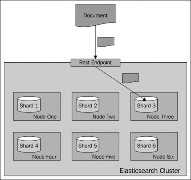
Default indexing
During indexing operations, when you send a document for indexing, Elasticsearch looks at its identifier to choose the shard in which the document should be indexed. By default, Elasticsearch calculates the hash value of the document's identifier and on the basis of that, it puts the document in one of the available primary shards. Then, those documents are redistributed to the replicas. The following diagram shows a simple illustration of how indexing works by default:
Default searching
Searching is a bit different from indexing, because in most situations, you need to query all the shards to get the data you are interested in. Imagine a situation when you have the following mappings describing your index:
{
"mappings" : {
"post" : {
"properties" : {
"id" : { "type" : "long", "store" : "yes",
"precision_step" : "0" },
"name" : { "type" : "string", "store" : "yes",
"index" : "analyzed" },
"contents" : { "type" : "string", "store" : "no",
"index" : "analyzed" },
"userId" : { "type" : "long", "store" : "yes",
"precision_step" : "0" }
}
}
}
}
As you can see, our index consists of four fields—the identifier (the id field), name of the document (the name field), contents of the document (the contents field), and the identifier of the user to which the documents belong (the userId field). To get all the documents for a particular user—one with userId equal to 12—you can run the following query:
curl –XGET 'http://localhost:9200/posts/_search?q=userId:12'
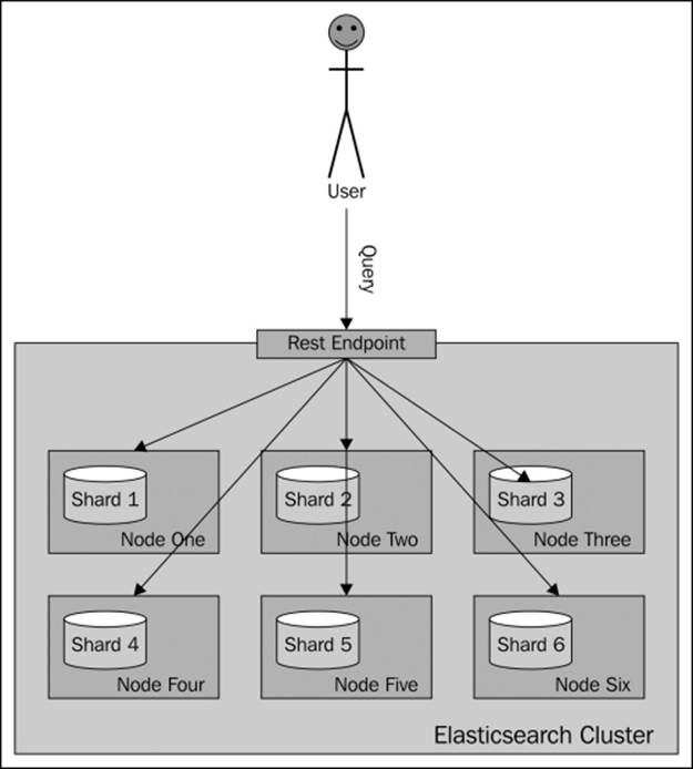
In general, you will send your query to one of the Elasticsearch nodes and Elasticsearch will do the rest. Depending on the search type (we will talk more about it in Chapter 3, Searching Your Data), Elasticsearch will run your query, which usually means that it will first query all the nodes for the identifier and score of the matching documents. Then, it will send an internal query again, but only to the relevant shards (the ones containing the needed documents) to get the documents needed to build the response.
A very simplified view of how default routing works during searching is shown in the following illustration:
What if we could put all the documents for a single user into a single shard and query on that shard? Wouldn't that be wise for performance? Yes, that is handy and that is what routing allows you do to.
Routing
Routing can control to which shard your documents and queries will be forwarded. By now, you will probably have guessed that we can specify the routing value both during indexing and during querying, and in fact if you decide to specify explicit routing values, you'll probably do that during indexing and searching.
In our case, we will use the userId value to set routing during indexing and the same value during searching. You can imagine that for the same userId value, the same hash value will be calculated and thus all the documents for that particular user will be placed in the same shard. Using the same value during search will result in searching a single shard instead of the whole index.
Remember that when using routing, you should still add a filter for the same value as the routing one. This is because you'll probably have more distinct routing values than the number of shards your index will be built with. Because of that, a few distinct values can point to the same shard, and if you omit filtering, you will get data not for a single value you route on, but for all those that reside in a particular shard.
The following diagram shows a very simple illustration of how searching works with a provided custom routing value:

As you can see, Elasticsearch will send our query to a single shard. Now let's look at how we can specify the routing values.
The routing parameters
The simplest way (but not always the most convenient one) is to provide the routing value using the routing parameter. When indexing or querying, you can add the routing parameter to your HTTP or set it by using the client library of your choice.
So, in order to index a sample document to the previously shown index, we will use the following lines of command:
curl -XPUT 'http://localhost:9200/posts/post/1?routing=12' -d '{
"id": "1",
"name": "Test document",
"contents": "Test document",
"userId": "12"
}'
This is how our previous query will look if we add the routing parameter:
curl -XGET 'http://localhost:9200/posts/_search?routing=12&q=userId:12'
As you can see, the same routing value was used during indexing and querying. We did that because we knew that during indexing we have used the value 12, so we wanted to point our query to the same shard and therefore we used exactly the same value.
Please note that you can specify multiple routing values separated by commas. For example, if we want the preceding query to be additionally routed with the use of the section parameter (if it existed) and we also want to filter by this parameter, our query will look like the following:
curl -XGET 'http://localhost:9200/posts/_search?routing=12,6654&q=userId:12+AND+section:6654'
Note
Remember that routing is not the only thing that is required to get results for a given user. That's because usually we have less shards that have unique routing values. This means that we will have data from multiple users in a single shard. So when using routing, you should also filter the results. You'll learn more about filtering in the Filtering your results section in Chapter 3, Searching Your Data.
Routing fields
Specifying the routing value with each request that we send to Elasticsearch works, but it is not convenient. In fact, Elasticsearch allows us to define a field whose value will be used as the routing value during indexing, so we only need to provide the routingparameter during querying. To do that, we need to add the following section to our type definition:
"_routing" : {
"required" : true,
"path" : "userId"
}
The preceding definition means that the routing value needs to be provided (the "required": true property); without it, an index request will fail. In addition to that, we specified the path attribute, which says which field value of the document will be used as the routing value. In our case, the userId field value will be used. These two parameters mean that each document we send for indexing needs to have the userId field defined. This is convenient, because we can now use batch indexing without the limitation of having all the documents from a single branch using the same routing value (which would be the case with the routing parameter). However, please remember that when using the routing field, Elasticsearch needs to do some additional parsing, and therefore it's a bit slower than when using the routing parameter.
After adding the routing part, the whole updated mappings file will be as follows:
{
"mappings" : {
"post" : {
"_routing" : {
"required" : true,
"path" : "userId"
},
"properties" : {
"id" : { "type" : "long", "store" : "yes",
"precision_step" : "0" },
"name" : { "type" : "string", "store" : "yes",
"index" : "analyzed" },
"contents" : { "type" : "string", "store" : "no",
"index" : "analyzed" },
"userId" : { "type" : "long", "store" : "yes",
"precision_step" : "0" }
}
}
}
}
If we want to create the posts index using the preceding mappings, use the following command to index a single, test document:
curl -XPOST 'localhost:9200/posts/post/1' -d '{
"id":1,
"name":"New post",
"contents": "New test post",
"userId":1234567
}'
Elasticsearch will end up using 1234567 as the routing value for indexing.
Summary
In this chapter, we learned how Elasticsearch indexing works. We learned to create our own mappings that define index structure and create indices using them. We learned what batch indexing is and how to use it, and how we can index our data efficiently. We also learned what additional information can be stored along with the documents. In addition to that, we've seen what segment merging is, how to configure it, and what throttling is. Finally, we used and configured routing.
In the next chapter, we will concentrate on searching. We will start with how to query Elasticsearch and what the basic queries we can use are. In addition to that, we will use filters and learn why they are important. We will see how we can validate our queries and how to use the highlighting functionality. Finally, we will use compound queries, we will get into querying internals, and we will sort our results.
All materials on the site are licensed Creative Commons Attribution-Sharealike 3.0 Unported CC BY-SA 3.0 & GNU Free Documentation License (GFDL)
If you are the copyright holder of any material contained on our site and intend to remove it, please contact our site administrator for approval.
© 2016-2026 All site design rights belong to S.Y.A.