Elasticsearch Server, Second Edition (2014)
Chapter 3. Searching Your Data
In the previous chapter, we learned how Elasticsearch indexing works, how to create our own mappings, and what data types we can use. We also stored additional information in our index and used routing, both default and nondefault. By the end of this chapter, we will have learned about the following topics:
· Querying Elasticsearch and choosing the data to be returned
· The working of the Elasticsearch querying process
· Understanding the basic queries exposed by Elasticsearch
· Filtering our results
· Understanding how highlighting works and how to use it
· Validating our queries
· Exploring compound queries
· Sorting our data
Querying Elasticsearch
So far, when we searched our data we used the REST API and a simple query or the GET request. Similarly, when we changed the index, we also used the REST API and sent the JSON-structured data to Elasticsearch, regardless of the type of operation we wanted to perform—whether it was a mapping change or document indexation. A similar situation happens when we want to send more than a simple query to Elasticsearch—we structure it using JSON objects and send it to Elasticsearch. This is called the query DSL. In a broader view, Elasticsearch supports two kinds of queries: basic ones and compound ones. Basic queries such as the term query are used for querying the actual data. We will cover these in the Basic queries section of this chapter. The second type of query is the compound query, such as the bool query, which can combine multiple queries. We will cover these in the Compound queries section of this chapter.
However, this is not the whole picture. In addition to these two types of queries, your query can have filter queries that are used to narrow down your results with certain criteria. Unlike other queries, filter queries don't affect scoring and are usually very efficient.
To make it even more complicated, queries can contain other queries. (Don't worry; we will try to explain this!) Furthermore, some queries can contain filters and others can contain both queries and filters. Although this is not everything, we will stick with this working explanation for now. We will go over this in detail in the Compound queries and Filtering your results sections of this chapter.
The example data
If not stated otherwise, the following mappings will be used for the rest of the chapter:
{
"book" : {
"_index" : {
"enabled" : true
},
"_id" : {
"index": "not_analyzed",
"store" : "yes"
},
"properties" : {
"author" : {
"type" : "string"
},
"characters" : {
"type" : "string"
},
"copies" : {
"type" : "long",
"ignore_malformed" : false
},
"otitle" : {
"type" : "string"
},
"tags" : {
"type" : "string"
},
"title" : {
"type" : "string"
},
"year" : {
"type" : "long",
"ignore_malformed" : false,
"index" : "analyzed"
},
"available" : {
"type" : "boolean"
}
}
}
}
Note
The string-based fields will be analyzed if not stated otherwise.
The preceding mappings (which are stored in the mapping.json file) were used to create the library index. In order to run them, use the following commands:
curl -XPOST 'localhost:9200/library'
curl -XPUT 'localhost:9200/library/book/_mapping' -d @mapping.json
If not stated otherwise, the following data will be used for the rest of the chapter:
{ "index": {"_index": "library", "_type": "book", "_id": "1"}}
{ "title": "All Quiet on the Western Front","otitle": "Im Westen nichts Neues","author": "Erich Maria Remarque","year": 1929,"characters": ["Paul Bäumer", "Albert Kropp", "Haie Westhus", "Fredrich Müller", "Stanislaus Katczinsky", "Tjaden"],"tags": ["novel"],"copies": 1, "available": true, "section" : 3}
{ "index": {"_index": "library", "_type": "book", "_id": "2"}}
{ "title": "Catch-22","author": "Joseph Heller","year": 1961,"characters": ["John Yossarian", "Captain Aardvark", "Chaplain Tappman", "Colonel Cathcart", "Doctor Daneeka"],"tags": ["novel"],"copies": 6, "available" : false, "section" : 1}
{ "index": {"_index": "library", "_type": "book", "_id": "3"}}
{ "title": "The Complete Sherlock Holmes","author": "Arthur Conan Doyle","year": 1936,"characters": ["Sherlock Holmes","Dr. Watson", "G. Lestrade"],"tags": [],"copies": 0, "available" : false, "section" : 12}
{ "index": {"_index": "library", "_type": "book", "_id": "4"}}
{ "title": "Crime and Punishment","otitle": "Преступлéние и наказáние","author": "Fyodor Dostoevsky","year": 1886,"characters": ["Raskolnikov", "Sofia Semyonovna Marmeladova"],"tags": [],"copies": 0, "available" : true}
We stored our data in the documents.json file, and we use the following command to index it:
curl -s -XPOST 'localhost:9200/_bulk' --data-binary @documents.json
This command runs bulk indexing. You can learn more about it in the Batch indexing to speed up your indexing process section in Chapter 2, Indexing Your Data.
A simple query
The simplest way to query Elasticsearch is to use the URI request query. We already discussed it in the Searching with the URI request query section of Chapter 1, Getting Started with the Elasticsearch Cluster. For example, to search for the word crime in the titlefield, send a query using the following command:
curl -XGET 'localhost:9200/library/book/_search?q=title:crime&pretty=true'
This is a very simple, but limited, way of submitting queries to Elasticsearch. If we look from the point of view of the Elasticsearch query DSL, the preceding query is the query_string query. It searches for the documents that have the crime term in the title field and can be rewritten as follows:
{
"query" : {
"query_string" : { "query" : "title:crime" }
}
}
Sending a query using the query DSL is a bit different, but still not rocket science. We send the GET HTTP request to the _search REST endpoint as before, and attach the query to the request body. Let's take a look at the following command:
curl -XGET 'localhost:9200/library/book/_search?pretty=true' -d '{
"query" : {
"query_string" : { "query" : "title:crime" }
}
}'
As you can see, we used the request body (the -d switch) to send the whole JSON-structured query to Elasticsearch. The pretty=true request parameter tells Elasticsearch to structure the response in such a way that we humans can read it more easily. In response to the preceding command, we get the following output:
{
"took" : 1,
"timed_out" : false,
"_shards" : {
"total" : 5,
"successful" : 5,
"failed" : 0
},
"hits" : {
"total" : 1,
"max_score" : 0.15342641,
"hits" : [ {
"_index" : "library",
"_type" : "book",
"_id" : "4",
"_score" : 0.15342641, "_source" : { "title": "Crime and Punishment","otitle": "
Преступлéние и наказáние","author": "Fyodor Dostoevsky","year": 1886,"characters": ["Raskolnikov", "Sofia Semyonovna Marmeladova"],"tags": [],"copies": 0, "available" : true}
} ]
}
}
Nice! We got our first search results with the query DSL.
Paging and result size
As we expected, Elasticsearch allows us to control how many results we want to get (at most) and from which result we want to start. The following are the two additional properties that can be set in the request body:
· from: This property specifies the document that we want to have our results from. Its default value is 0, which means that we want to get our results from the first document.
· size: This property specifies the maximum number of documents we want as the result of a single query (which defaults to 10). For example, if we are only interested in faceting results and don't care about the documents returned by the query, we can set this parameter to 0.
If we want our query to get documents starting from the tenth item on the list and get 20 of items from there on, we send the following query:
{
"from" : 9,
"size" : 20,
"query" : {
"query_string" : { "query" : "title:crime" }
}
}
Tip
Downloading the example code
You can download the example code files for all Packt books you have purchased from your account at http://www.PacktPub.com. If you purchased this book elsewhere, you can visit http://www.PacktPub.com/support and register to have the files e-mailed directly to you.
Returning the version value
In addition to all the information returned, Elasticsearch can return the version of the document. To do this, we need to add the version property with the value of true to the top level of our JSON object. So, the final query, which requests for version information, will look as follows:
{
"version" : true,
"query" : {
"query_string" : { "query" : "title:crime" }
}
}
After running the preceding query, we get the following results:
{
"took" : 2,
"timed_out" : false,
"_shards" : {
"total" : 5,
"successful" : 5,
"failed" : 0
},
"hits" : {
"total" : 1,
"max_score" : 0.15342641,
"hits" : [ {
"_index" : "library",
"_type" : "book",
"_id" : "4",
"_version" : 1,
"_score" : 0.15342641, "_source" : { "title": "Crime and Punishment","otitle": "
Преступлéние и наказáние","author": "Fyodor Dostoevsky","year": 1886,"characters": ["Raskolnikov", "Sofia Semyonovna Marmeladova"],"tags": [],"copies": 0, "available" : true}
} ]
}
}
As you can see, the _version section is present for the single hit we got.
Limiting the score
For nonstandard use cases, Elasticsearch provides a feature that lets us filter the results on the basis of the minimum score value that the document must have to be considered a match. In order to use this feature, we must provide the min_score value at the top level of our JSON object with the value of the minimum score. For example, if we want our query to only return documents with a score higher than 0.75, we send the following query:
{
"min_score" : 0.75,
"query" : {
"query_string" : { "query" : "title:crime" }
}
}
We get the following response after running the preceding query:
{
"took" : 1,
"timed_out" : false,
"_shards" : {
"total" : 5,
"successful" : 5,
"failed" : 0
},
"hits" : {
"total" : 0,
"max_score" : null,
"hits" : [ ]
}
}
If you look at the previous examples, the score of our document was 0.15342641, which is lower than 0.75, and thus we didn't get any documents in response.
Limiting the score doesn't make much sense, usually because comparing scores between queries is quite hard. However, maybe in your case, this functionality will be needed.
Choosing the fields that we want to return
With the use of the fields array in the request body, Elasticsearch allows us to define which fields to include in the response. Remember that you can only return those fields if they are marked as stored in the mappings used to create the index, or if the _source field was used (Elasticsearch uses the _source field to provide the stored values). So, for example, to return only the title and year fields in the results (for each document), send the following query to Elasticsearch:
{
"fields" : [ "title", "year" ],
"query" : {
"query_string" : { "query" : "title:crime" }
}
}
And in response, we get the following output:
{
"took" : 2,
"timed_out" : false,
"_shards" : {
"total" : 5,
"successful" : 5,
"failed" : 0
},
"hits" : {
"total" : 1,
"max_score" : 0.15342641,
"hits" : [ {
"_index" : "library",
"_type" : "book",
"_id" : "4",
"_score" : 0.15342641,
"fields" : {
"title" : [ "Crime and Punishment" ],
"year" : [ 1886 ]
}
} ]
}
}
As you can see, everything worked as we wanted it to. There are three things we would like to share with you, which are as follows:
· If we don't define the fields array, it will use the default value and return the _source field if available
· If we use the _source field and request a field that is not stored, then that field will be extracted from the _source field (however, this requires additional processing)
· If we want to return all stored fields, we just pass an asterisk (*) as the field name
Note
From a performance point of view, it's better to return the _source field instead of multiple stored fields.
The partial fields
In addition to choosing which fields are returned, Elasticsearch allows us to use the so-called partial fields. They allow us to control how fields are loaded from the _source field. Elasticsearch exposes the include and exclude properties of the partial_fields object so we can include and exclude fields on the basis of these properties. For example, for our query to include the fields that start with titl and exclude the ones that start with chara, we send the following query:
{
"partial_fields" : {
"partial1" : {
"include" : [ "titl*" ],
"exclude" : [ "chara*" ]
}
},
"query" : {
"query_string" : { "query" : "title:crime" }
}
}
Using the script fields
Elasticsearch allows us to use script-evaluated values that will be returned with result documents. To use the script fields, we add the script_fields section to our JSON query object and an object with a name of our choice for each scripted value that we want to return. For example, to return a value named correctYear, which is calculated as the year field minus 1800, we run the following query:
{
"script_fields" : {
"correctYear" : {
"script" : "doc['year'].value - 1800"
}
},
"query" : {
"query_string" : { "query" : "title:crime" }
}
}
Using the doc notation, like we did in the preceding example, allows us to catch the results returned, which thereby results in faster script execution, but it also leads to higher memory consumption. We are also limited to single-valued and single term fields. If we care about memory usage, or we are using more complicated field values, we can always use the _source field. Our query using this field looks as follows:
{
"script_fields" : {
"correctYear" : {
"script" : "_source.year - 1800"
}
},
"query" : {
"query_string" : { "query" : "title:crime" }
}
}
The following response is returned by Elasticsearch for the preceding query:
{
"took" : 1,
"timed_out" : false,
"_shards" : {
"total" : 5,
"successful" : 5,
"failed" : 0
},
"hits" : {
"total" : 1,
"max_score" : 0.15342641,
"hits" : [ {
"_index" : "library",
"_type" : "book",
"_id" : "4",
"_score" : 0.15342641,
"fields" : {
"correctYear" : [ 86 ]
}
} ]
}
}
As you can see, we got the calculated correctYear field in response.
Passing parameters to the script fields
Let's take a look at one more feature of the script fields: the passing of additional parameters. Instead of having the value 1800 in the equation, we can use a variable name and pass its value in the params section. If we do this, our query will look as follows:
{
"script_fields" : {
"correctYear" : {
"script" : "_source.year - paramYear",
"params" : {
"paramYear" : 1800
}
}
},
"query" : {
"query_string" : { "query" : "title:crime" }
}
}
As you can see, we added the paramYear variable as a part of the scripted equation and provided its value in the params section.
You can learn more about the use of scripts in the Scripting capabilities of Elasticsearch section of Chapter 5, Make Your Search Better.
Understanding the querying process
After reading the previous section, we now know how querying works in Elasticsearch. You know that Elasticsearch, in most cases, needs to scatter the query across multiple nodes, get the results, merge them, fetch for relevant documents, and return the results. What we didn't talk about is three additional things that define how queries behave: query rewrite, search type, and query execution preference. We will now concentrate on these functionalities of Elasticsearch and also try to show you how querying works.
Query logic
Elasticsearch is a distributed search engine, and so all functionality provided must be distributed in its nature. It is exactly the same with querying. Since we want to discuss some more advanced topics on how to control the query process, we first need to know how it works.
By default, if we don't alter anything, the query process will consist of two phases as shown in the following diagram:
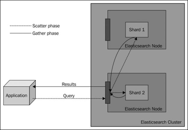
When we send a query, we send it to one of the Elasticsearch nodes. What is occurring now is a so-called scatter phase. The query is distributed to all the shards that our index is built of. For example, if it is built of five shards and one replica, then five physical shards will be queried (we don't need to query both a shard and its replica because they contain the same data). Each of the queried shards will only return the document identifier and the score of the document. The node that sent the scatter query will wait for all the shards to complete their task, gather the results, and sort them appropriately (in this case, from the top scoring to the lowest scoring ones).
After that, a new request will be sent to build the search results. However, for now, the request will be sent only to those shards that held the documents to build the response. In most cases, Elasticsearch won't send the request to all the shards but only to its subset. This is because we usually don't get the entire result of the query but only a portion of it. This phase is called the gather phase. After all the documents have been gathered, the final response is built and returned as the query result.
Of course, the preceding behavior is the default in Elasticsearch and can be altered. The following section will describe how to change this behavior.
Search types
Elasticsearch allows us to choose how we want our query to be processed internally. We can do this by specifying the search type. There are different situations where different search types are appropriate; you may only care about performance, while sometimes, query relevance may be the most important factor. You should remember that each shard is a small Lucene index, and in order to return more relevant results, some information, such as frequencies, needs to be transferred between shards. To control how queries are executed, we can pass the search_type request parameter and set it to one of the following values:
· query_then_fetch: In the first step, the query is executed to get the information needed to sort and rank the documents. This step is executed against all the shards. Then, only the relevant shards are queried for the actual content of the documents. Different from query_and_fetch, the maximum number of results returned by this query type will be equal to the size parameter. This is the search type used by default if no search type has been provided with the query, and this is the query type we described earlier.
· query_and_fetch: This is usually the fastest and simplest search type implementation. The query is executed against all the shards (of course, only a single replica of a given primary shard will be queried) in parallel, and all the shards return the number of results equal to the value of the size parameter. The maximum number of returned documents will be equal to the value of size multiplied by the number of shards.
· dfs_query_and_fetch: This is similar to the query_and_fetch search type, but it contains an additional phase compared to query_and_fetch. The additional part is the initial query phase that is executed to calculate distributed term frequencies to allow more precise scoring of returned documents and thus more relevant query results.
· dfs_query_then_fetch: As with the previous dfs_query_and_fetch search type, the dfs_query_then_fetch search type is similar to its counterpart: query_then_fetch. However, it contains an additional phase compared to query_then_fetch, just like dfs_query_and_fetch.
· count: This is a special search type that only returns the number of documents that matched the query. If you only need to get the number of results but do not care about the documents, you should use this search type.
· scan: This is another special search type. Only use it if you expect your query to return a large amount of results. It differs a bit from the usual queries because after sending the first request, Elasticsearch responds with a scroll identifier, similar to a cursor in relational databases. All the queries need to be run against the _search/scroll REST endpoint and need to send the returned scroll identifier in the request body. You can learn more about this functionality in the The scroll API section of Chapter 6, Beyond Full-text Searching.
So if we want to use the simplest search type, we run the following command:
curl -XGET 'localhost:9200/library/book/_search?pretty=true&search_type=query_and_fetch' -d '{
"query" : {
"term" : { "title" : "crime" }
}
}'
Search execution preferences
In addition to the possibility of controlling how the query is executed, we can also control the shards that we want to execute the query on. By default, Elasticsearch uses shards and replicas, both the ones available on the node that we've sent the request on and the other nodes in the cluster. And, the default behavior is in most cases the best query preference method. However, there may be times when we want to change the default behavior. For example, we may want the search to be executed on only the primary shards. To do this, we can set the preference request parameter to one of the following values shown in the table:
|
Parameter values |
Description |
|
_primary |
This search operation will only be executed on the primary shards, so the replicas won't be used. This can be useful when we need to use the latest information from the index, but our data is not replicated right away. |
|
_primary_first |
This search operation will be executed on the primary shards if they are available. If not, it will be executed on the other shards. |
|
_local |
This search operation will only be executed on the shards available on the node that we are sending the request to (if possible). |
|
_only_node:node_id |
This search operation will be executed on the node with the provided node identifier. |
|
_prefer_node:node_id |
Elasticsearch will try to execute this search operation on the node with the provided identifier. However, if the node is not available, it will be executed on the nodes that are available. |
|
_shards:1,2 |
Elasticsearch will execute the operation on the shards with the given identifiers (in this case, on the shards with the identifiers 1 and 2). The _shards parameter can be combined with other preferences, but the shard identifiers need to be provided first, for example, _shards:1,2;_local. |
|
Custom value |
Any custom string value may be passed. The requests provided with the same values will be executed on the same shards. |
For example, if we want to execute a query only on the local shards, we run the following command:
curl -XGET 'localhost:9200/library/_search?preference=_local' -d '{
"query" : {
"term" : { "title" : "crime" }
}
}'
The Search shards API
When discussing the search preference, we would also like to mention the Search shards API exposed by Elasticsearch. This API allows us to check the shards that the query will be executed on. In order to use this API, run a request against the _search_shardsREST endpoint. For example, to see how the query is executed, we run the following command:
curl -XGET 'localhost:9200/library/_search_shards?pretty' -d '{"query":"match_all":{}}'
And, the response to the preceding command is as follows:
{
"nodes" : {
"N0iP_bH3QriX4NpqsqSUAg" : {
"name" : "Oracle",
"transport_address" : "inet[/192.168.1.19:9300]"
}
},
"shards" : [ [ {
"state" : "STARTED",
"primary" : true,
"node" : "N0iP_bH3QriX4NpqsqSUAg",
"relocating_node" : null,
"shard" : 0,
"index" : "library"
} ], [ {
"state" : "STARTED",
"primary" : true,
"node" : "N0iP_bH3QriX4NpqsqSUAg",
"relocating_node" : null,
"shard" : 1,
"index" : "library"
} ], [ {
"state" : "STARTED",
"primary" : true,
"node" : "N0iP_bH3QriX4NpqsqSUAg",
"relocating_node" : null,
"shard" : 4,
"index" : "library"
} ], [ {
"state" : "STARTED",
"primary" : true,
"node" : "N0iP_bH3QriX4NpqsqSUAg",
"relocating_node" : null,
"shard" : 3,
"index" : "library"
} ], [ {
"state" : "STARTED",
"primary" : true,
"node" : "N0iP_bH3QriX4NpqsqSUAg",
"relocating_node" : null,
"shard" : 2,
"index" : "library"
} ] ]
}
As you can see, in the response returned by Elasticsearch, we have the information about the shards that will be used during the query process. Of course, with the Search shards API, you can use all the parameters, such as routing or preference, and see how it affects your search execution.
Basic queries
Elasticsearch has extensive search and data analysis capabilities that are exposed in the form of different queries, filters, and aggregates, and so on. In this section, we will concentrate on the basic queries provided by Elasticsearch.
The term query
The term query is one of the simplest queries in Elasticsearch. It just matches the document that has a term in a given field—the exact, not analyzed term. The simplest term query is as follows:
{
"query" : {
"term" : {
"title" : "crime"
}
}
}
The preceding query will match the documents that have the crime term in the title field. Remember that the term query is not analyzed, so you need to provide the exact term that will match the term in the indexed document. Please note that in our input data, we have the title field with the Crime and Punishment term, but we are searching for crime because the Crime term becomes crime after analysis during indexing.
In addition to the term we want to find, we can also include the boost attribute to our term query; it will affect the importance of the given term. We will talk more about boosts in the An introduction to Apache Lucene scoring section of Chapter 5, Make Your Search Better. For now, we just need to remember that it changes the importance of the given part of the query.
For example, to change our previous query and give a boost of 10.0 to our term query, we send the following query:
{
"query" : {
"term" : {
"title" : {
"value" : "crime",
"boost" : 10.0
}
}
}
}
As you can see, the query changed a bit. Instead of a simple term value, we nested a new JSON object that contains the value property and the boost property. The value of the value property contains the term we are interested in, and the boost property is the boost value we want to use.
The terms query
The terms query allows us to match documents that have certain terms in their contents. The term query allowed us to match a single, not analyzed term, and the terms query allows us to match multiples of these. For example, let's say that we want to get all the documents that have the terms novel or book in the tags field. To achieve this, we run the following query:
{
"query" : {
"terms" : {
"tags" : [ "novel", "book" ],
"minimum_match" : 1
}
}
}
The preceding query returns all the documents that have one or both of the searched terms in the tags field. Why is that? It is because we set the minimum_match property to 1; this basically means that one term should match. If we want the query to match the document with all the provided terms, we set the minimum_match property to 2.
The match_all query
The match_all query is one of the simplest queries available in Elasticsearch. It allows us to match all the documents in the index. If we want to get all the documents from our index, we just run the following query:
{
"query" : {
"match_all" : {}
}
}
We can also include boost in the query, which will be given to all the documents matched by it. For example, if we want to add a boost of 2.0 to all the documents in our match_all query, we send the following query to Elasticsearch:
{
"query" : {
"match_all" : {
"boost" : 2.0
}
}
}
The common terms query
The common terms query is a modern Elasticsearch solution for improving query relevance and precision with common words when we are not using stop words (http://en.wikipedia.org/wiki/Stop_words). For example, crime and punishment can be translated to three term queries and each of those term queries have a cost in terms of performance (the more the terms, the lower the performance of the query). However, the and term is a very common one, and its impact on the document score will be very low. The solution is the common terms query that divides the query into two groups. The first group is the one with important terms; these are the ones that have lower frequency. The second group is the less important terms that have higher frequency. The first query is executed first, and Elasticsearch calculates the score for all the terms from the first group. This way, the low frequency terms, which are usually the ones that have more importance, are always taken into consideration. Then, Elasticsearch executes the second query for the second group of terms but calculates the score only for the documents that were matched for the first query. This way, the score is only calculated for the relevant documents and thus, higher performance is achieved.
An example of the common terms query is as follows:
{
"query" : {
"common" : {
"title" : {
"query" : "crime and punishment",
"cutoff_frequency" : 0.001
}
}
}
}
The query can take the following parameters:
· query: This parameter defines the actual query contents.
· cutoff_frequency: This parameter defines the percentage (0.001 means 0.1 percent) or an absolute value (when the property is set to a value equal to or larger than 1). High and low frequency groups are constructed using this value. Setting this parameter to0.001 means that the low frequency terms group will be constructed for terms that have a frequency of 0.1 percent and lower.
· low_freq_operator: This parameter can be set to or or and (defaults to or). It specifies the Boolean operator used to construct queries in the low frequency term group. If we want all of the terms to be present in a document for it to be considered a match, we should set this parameter to and.
· high_freq_operator: This parameter can be set to or or and (it defaults to or). It specifies the Boolean operator used to construct queries in the high frequency term group. If we want all of the terms to be present in a document for it to be considered a match, we should set this parameter to and.
· minimum_should_match: Instead of using the low_freq_operator and high_freq_operator parameters, we can use minimum_should_match. Just like with other queries, it allows us to specify the minimum number of terms that should be found in a document for it to be considered a match.
· boost: This parameter defines the boost given to the score of the documents.
· analyzer: This parameter defines the name of the analyzer that will be used to analyze the query text and defaults to the default analyzer.
· disable_coord: This parameter value defaults to false and allows us to enable or disable the score factor computation that is based on the fraction of all the query terms that a document contains. Set it to true for less precise scoring but slightly faster queries.
Note
Unlike the term and terms queries, the common terms query is analyzed by Elasticsearch.
The match query
The match query takes the values given in the query parameter, analyzes them, and constructs the appropriate query out of them. When using a match query, Elasticsearch will choose the proper analyzer for a field we've chosen, so we can be sure that the terms passed to the match query will be processed by the same analyzer that was used during indexing. Please remember that the match query (and the multi_match query that will be explained later) doesn't support the Lucene query syntax; however, it fits perfectly as a query handler for our search box. The simplest match (and the default) query can look like the following:
{
"query" : {
"match" : {
"title" : "crime and punishment"
}
}
}
The preceding query will match all the documents that have the terms, crime, and, or punishment in the title field. However, the previous query is only the simplest one; there are multiple types of match queries that we will discuss now.
The Boolean match query
The Boolean match query is a query that analyzes the provided text and makes a Boolean query out of it. There are a few parameters that allow us to control the behavior of the Boolean match queries; they are as follows:
· operator: This parameter can take the value of or or and and control the Boolean operator that is used to connect the created Boolean clauses. The default value is or. If we want all the terms in our query to match, we use the and Boolean operator.
· analyzer: This parameter specifies the name of the analyzer that will be used to analyze the query text and defaults to the default analyzer.
· fuzziness: Providing the value of this parameter allows us to construct fuzzy queries. It should take values from 0.0 to 1.0 for a string type. While constructing fuzzy queries, this parameter will be used to set the similarity.
· prefix_length: This parameter allows us to control the behavior of the fuzzy query. For more information on the value of this parameter, refer to the The fuzzy_like_this query section in this chapter.
· max_expansions: This parameter allows us to control the behavior of the fuzzy query. For more information on the value of this parameter, please refer to the The fuzzy_like_this query section in this chapter.
· zero_terms_query: This parameter allows us to specify the behavior of the query when all the terms are removed by the analyzer (for example, because of stop words). It can be set to none or all, with none as the default value. When set to none, no documents will be returned when the analyzer removes all the query terms. All the documents will be returned on setting this parameter to all.
· cutoff_frequency: This parameter allows us to divide the query into two groups: one with high frequency terms and one with low frequency terms. Refer to the description of the common terms query to see how this parameter can be used.
The parameters should be wrapped in the name of the field that we are running the query for. So if we wish to run a sample Boolean match query against the title field, we send a query as follows:
{
"query" : {
"match" : {
"title" : {
"query" : "crime and punishment",
"operator" : "and"
}
}
}
}
The match_phrase query
A match_phrase query is similar to the Boolean query, but instead of constructing the Boolean clauses from the analyzed text, it constructs the phrase query. The following parameters are available for this query:
· slop: This is an integer value that defines how many unknown words can be put between terms in the text query for a match to be considered a phrase. The default value of this parameter is 0, which means that no additional words are allowed.
· analyzer: This parameter specifies the name of the analyzer that will be used to analyze the query text and defaults to the default analyzer.
A sample match_phrase query against the title field looks like the following code:
{
"query" : {
"match_phrase" : {
"title" : {
"query" : "crime punishment",
"slop" : 1
}
}
}
}
Note that we removed the and term from our query, but since the slop parameter is set to 1, it will still match our document.
The match_phrase_prefix query
The last type of the match query is the match_phrase_prefix query. This query is almost the same as the match_phrase query, but in addition, it allows prefix matches on the last term in the query text. Also, in addition to the parameters exposed by the match_phrasequery, it exposes an additional one: the max_expansions parameter. This controls how many prefixes will be rewritten to the last terms. Our example query when changed to the match_phrase_prefix query will look like the following:
{
"query" : {
"match_phrase_prefix" : {
"title" : {
"query" : "crime and punishm",
"slop" : 1,
"max_expansions" : 20
}
}
}
}
Note that we didn't provide the full crime and punishment phrase but only crime and punishm, and the query still matches our document.
The multi_match query
The multi_match query is the same as the match query, but instead of running against a single field, it can be run against multiple fields with the use of the fields parameter. Of course, all the parameters you use with the match query can be used with the multi_matchquery. So, if we want to modify our match query to be run against the title and otitle fields, we run the following query:
{
"query" : {
"multi_match" : {
"query" : "crime punishment",
"fields" : [ "title", "otitle" ]
}
}
}
In addition to the previously mentioned parameters, the multi_match query exposes the following additional parameters that allow more control over its 'margin-left:18.0pt;text-indent:-18.0pt;line-height: normal'>· use_dis_max: This parameter defines the Boolean value that allows us to set whether the dismax (true) or boolean (false) queries should be used. It defaults to true. You can read more about the dismax query in the The dismax query section of this chapter.
· tie_breaker: This parameter is only used when the use_dis_max parameter is set to true and allows us to specify the balance between lower and maximum scoring query items. You can read more about it in the The dismax query section of this chapter.
The query_string query
In comparison to the other queries available, the query_string query supports the full Apache Lucene query syntax, which we discussed earlier in the The Lucene query syntax section in Chapter 1, Getting Started with the Elasticsearch Cluster. It uses a query parser to construct an actual query using the provided text. An example of the query_string query is as follows:
{
"query" : {
"query_string" : {
"query" : "title:crime^10 +title:punishment -otitle:cat +author:(+Fyodor +dostoevsky)",
"default_field" : "title"
}
}
}
Because we are familiar with the basics of the Lucene query syntax, we can discuss how the preceding query works. As you can see, we wanted to get the documents that may have the term crime in the title field, and such documents should be boosted with the value of 10. Next, we want only the documents that have the punishment term in the title field and not the documents with the cat term in the otitle field. Finally, we tell Lucene that we only want the documents that have the Fyodor and dostoevsky terms in the authorfield.
Like most of the queries in Elasticsearch, the query_string query provides the following parameters that allow us to control the query 'margin-left:18.0pt;text-indent:-18.0pt;line-height: normal'>· query: This parameter specifies the query text.
· default_field: This parameter specifies the default field that the query will be executed against. It defaults to the index.query.default_field property, which is set to _all by default.
· default_operator: This parameter specifies the default logical operator (or or and) that is used when no operator is specified. The default value of this parameter is or.
· analyzer: This parameter specifies the name of the analyzer that is used to analyze the query provided in the query parameter.
· allow_leading_wildcard: This parameter specifies whether a wildcard character is allowed as the first character of a term. It defaults to true.
· lowercase_expand_terms: This parameter specifies whether the terms that are a result of a query rewrite should be lowercased. It defaults to true, which means that the rewritten terms will be lowercased.
· enable_position_increments: This parameter specifies whether the position increments should be turned on in the result query. It defaults to true.
· fuzzy_max_expansions: This parameter specifies the maximum terms that the fuzzy query will be expanded into if used. It defaults to 50.
· fuzzy_prefix_length: This parameter specifies the prefix length for the generated fuzzy queries and defaults to 0. To learn more about it, refer to the The fuzzy query section.
· fuzzy_min_sim: This parameter specifies the minimum similarity for the fuzzy queries and defaults to 0.5. To learn more about it, refer to the The fuzzy query section.
· phrase_slop: This parameter specifies the phrase slop value and defaults to 0. To learn more about it, refer to the The match_phrase query section.
· boost: This parameter specifies the boost value that will be used and defaults to 1.0.
· analyze_wildcard: This parameter specifies whether the terms generated by the wildcard query should be analyzed. It defaults to false, which means that the terms won't be analyzed.
· auto_generate_phrase_queries: This parameter specifies whether phrase queries will be generated from the query automatically. It defaults to false, which means that the phrase queries won't be generated automatically.
· minimum_should_match: This parameter controls how many generated Boolean should clauses must match against a document for it to be consider a hit. The value can be provided as a percentage, for example, 50%. This means that at least 50 percent of the given terms should match. It can also be provided as an integer value, such as 2, which means that at least two terms must match.
· lenient: This parameter takes the value of true or false. If set to true, format-based failures will be ignored.
DisMax is an abbreviation of Disjunction Max. Disjunction refers to the fact that the search is executed across multiple fields, and the fields can be given different boost weights. Max means that only the maximum score for a given term will be included in a final document score and not the sum of all the scores from all fields that have the matched term (like a simple Boolean query would do).
Note that Elasticsearch can rewrite the query_string query, and because of this, Elasticsearch allows us to pass additional parameters that control the rewrite method. However, for more details on this process, refer to the Understanding the querying process section in this chapter.
Running the query_string query against multiple fields
It is possible to run the query_string query against multiple fields. In order to do this, one needs to provide the fields parameter in the query body, which holds the array of field names. There are two methods of running the query_string query against multiple fields; the default method uses the Boolean query to make queries and the other method uses the dismax query.
In order to use the dismax query, you should add the use_dis_max property in the query body and set it to true. An example query is as follows:
{
"query" : {
"query_string" : {
"query" : "crime punishment",
"fields" : [ "title", "otitle" ],
"use_dis_max" : true
}
}
}
The simple_query_string query
The simple_query_string query uses one of the newest query parsers in Lucene: SimpleQueryParser. Similar to the query_string query, it accepts the Lucene query syntax as the query; however unlike it, the simple_query_string query never throws an exception when an error is parsed. Instead of throwing an exception, it discards the invalid parts of the query and runs the rest of the parts.
An example of the simple_query_string query is as follows:
{
"query" : {
"simple_query_string" : {
"query" : "title:crime^10 +title:punishment -otitle:cat +author:(+Fyodor +dostoevsky)",
"default_operator" : "and"
}
}
}
This query supports parameters similar to the ones exposed by the query_string query, and similarly, it can also be run against multiple fields using the fields property.
The identifiers query
The identifiers query is a simple query that filters the returned documents to only those queries with provided identifiers. This query works on the internal _uid field, so it doesn't require the _id field to be enabled. The simplest version of such a query looks like the following:
{
"query" : {
"ids" : {
"values" : [ "10", "11", "12", "13" ]
}
}
}
This query only returns documents that have one of the identifiers present in the values array. We can complicate the identifiers query a bit and also limit the documents on the basis of their type. For example, if we want to only include documents from the book type, we send the following query:
{
"query" : {
"ids" : {
"type" : "book",
"values" : [ "10", "11", "12", "13" ]
}
}
}
As you can see, we added the type property to our query and set its value to the type we are interested in.
The prefix query
The prefix query is similar to the term query in terms of its configuration. The prefix query allows us to match documents that have the value in a certain field and starts with a given prefix. For example, if we want to find all the documents that have values starting with cri in the title field, we run the following query:
{
"query" : {
"prefix" : {
"title" : "cri"
}
}
}
Similar to the term query, we can also include the boost attribute to our prefix query; this will affect the importance of the given prefix. For example, if we want to change our previous query and give it a boost of 3.0, we send the following query:
{
"query" : {
"prefix" : {
"title" : {
"value" : "cri",
"boost" : 3.0
}
}
}
}
Note
The prefix query is rewritten by Elasticsearch; therefore, Elasticsearch allows us to pass an additional parameter by controlling the rewrite method. However, for more details on this process, refer to the Understanding the querying process section of this chapter.
The fuzzy_like_this query
The fuzzy_like_this query is similar to the more_like_this query. It finds all the documents that are similar to the provided text, but it works a bit differently than the more_like_this query. It makes use of fuzzy strings and picks the best differencing terms that were produced. For example, if we want to run a fuzzy_like_this query against the title and otitle fields to find all the documents similar to the crime punishment query, we run the following query:
{
"query" : {
"fuzzy_like_this" : {
"fields" : ["title", "otitle"],
"like_text" : "crime punishment"
}
}
}
The following query parameters are supported by the fuzzy_like_this query:
· fields: This parameter defines an array of fields against which the query should be run. It defaults to the _all field.
· like_text: This is a required parameter that holds the text that we compare the documents to.
· ignore_tf: This parameter specifies whether term frequencies should be ignored during similarity computation. It defaults to false, which means that the term frequencies will be used.
· max_query_terms: This parameter specifies the maximum number of query terms that will be included in a generated query. It defaults to 25.
· min_similarity: This parameter specifies the minimum similarity that differencing terms should have. It defaults to 0.5.
· prefix_length: This parameter specifies the length of the common prefix of the differencing terms. It defaults to 0.
· boost: This parameter specifies the boost value that will be used when boosting a query. It defaults to 1.0.
· analyzer: This parameter specifies the name of the analyzer that will be used to analyze the text we provided.
The fuzzy_like_this_field query
The fuzzy_like_this_field query is similar to the fuzzy_like_this query, but it only works against a single field. Because of this, it doesn't support the fields property. Instead of specifying the fields that should be used for query analysis, we should wrap the query parameters into that field name. Our example query to a title field should look like the following:
{
"query" : {
"fuzzy_like_this_field" : {
"title" : {
"like_text" : "crime and punishment"
}
}
}
}
All the other parameters from the fuzzy_like_this_field query work the same for this query.
The fuzzy query
The fuzzy query is the third type of fuzzy query; it matches the documents on the basis of the edit distance algorithm. The edit distance is calculated on the basis of terms we provide in the query and against the searched documents. This query can be expensive when it comes to CPU resources, but it can help us when we need fuzzy matching, for example, when users make spelling mistakes. In our example, let's assume that instead of crime, our user enters the word crme into the search box and we want to run the simplest form of fuzzy query. Such a query would look like the following:
{
"query" : {
"fuzzy" : {
"title" : "crme"
}
}
}
And, the response for such a query would be as follows:
{
"took" : 1,
"timed_out" : false,
"_shards" : {
"total" : 5,
"successful" : 5,
"failed" : 0
},
"hits" : {
"total" : 1,
"max_score" : 0.15342641,
"hits" : [ {
"_index" : "library",
"_type" : "book",
"_id" : "4",
"_score" : 0.15342641, "_source" : { "title": "Crime and Punishment","otitle": "
Преступлéние и наказáние","author": "Fyodor Dostoevsky","year": 1886,"characters": ["Raskolnikov", "Sofia Semyonovna Marmeladova"],"tags": [],"copies": 0, "available" : true}
} ]
}
}
Even though we made a typo, Elasticsearch managed to find the documents we were interested in.
We can control the behavior of the fuzzy query using the following parameters:
· value: This parameter specifies the actual query.
· boost: This parameter specifies the boost value for the query. It defaults to 1.0.
· min_similarity: This parameter specifies the minimum similarity a term must have to count as a match. In the case of string fields, this value should be between 0 and 1 inclusive. For numeric fields, this value can be greater than one; for example, if the query value is equal to 20 and min_similarity is set to 3, we get values from 17 to 23. For date fields, we can have the min_similarity values that include 1d, 2d, 1m, and so on. These values correspond to one day, two days, and one month, respectively.
· prefix_length: This parameter defines the length of the common prefix of the differencing terms; it defaults to 0.
· max_expansions: This parameter specifies the maximum number of terms that the query will be expanded to. The default value is unbounded.
The parameters should be wrapped in the name of the field that we are running the query against. So if we want to modify the previous query and add additional parameters, the query will look like the following code:
{
"query" : {
"fuzzy" : {
"title" : {
"value" : "crme",
"min_similarity" : 0.2
}
}
}
}
The wildcard query
The wildcard query allows us to use the * and ? wildcards in the values that we search for. Apart from this, the wildcard query is very similar to the term query in terms of its content. To send a query that matches all the documents with the value of the cr?me term, where ? means any character, we send the following query:
{
"query" : {
"wildcard" : {
"title" : "cr?me"
}
}
}
This will match the documents that have all the terms that match cr?me in the title field. However, you can also include the boost attribute to your wildcard query; it will affect the importance of each term that matches the given value. For example, if we want to change our previous query and give a boost of 20.0 to our term query, we send the following query:
{
"query" : {
"wildcard" : {
"title" : {
"value" : "cr?me",
"boost" : 20.0
}
}
}
}
Note
Note that wildcard queries are not very performance-oriented queries and should be avoided if possible; in particular, avoid leading wildcards (the terms that start with wildcards). Also, note that the wildcard query is rewritten by Elasticsearch, and because of this, Elasticsearch allows us to pass an additional parameter that controls the rewrite method. For more details on this process, refer to the Understanding the querying process section of this chapter.
The more_like_this query
The more_like_this query allows us to get documents that are similar to the provided text. Elasticsearch supports a few parameters to define how the more_like_this query should work; they are as follows:
· fields: This parameter defines an array of fields that the query should be run against. It defaults to the _all field.
· like_text: This is a required parameter that holds the text that we compare the documents to.
· percent_terms_to_match: This parameter specifies the percentage of terms from the query that need to match in a document for that document to be considered similar. It defaults to 0.3, which means 30 percent.
· min_term_freq: This parameter specifies the minimum term frequency (for the terms in the documents) below which terms will be ignored. It defaults to 2.
· max_query_terms: This parameter specifies the maximum number of terms that will be included in any generated query. It defaults to 25. A higher value may mean higher precision, but lower performance.
· stop_words: This parameter defines an array of words that will be ignored when comparing the documents and the query. It is empty by default.
· min_doc_freq: This parameter defines the minimum number of documents in which the term has to be present to not be ignored. It defaults to 5, which means that a term needs to be present in at least five documents.
· max_doc_freq: This parameter defines the maximum number of documents in which a term may be present in order to not be ignored. By default, it is unbounded.
· min_word_len: This parameter defines the minimum length of a single word below which the word will be ignored. It defaults to 0.
· max_word_len: This parameter defines the maximum length of a single word above which the word will be ignored. It is unbounded by default.
· boost_terms: This parameter defines the boost value that will be used to boost each term. It defaults to 1.
· boost: This parameter defines the boost value that will be used to boost the query. It defaults to 1.
· analyzer: This parameter defines the name of the analyzer that will be used to analyze the text we provided.
An example of the more_like_this query is as follows:
{
"query" : {
"more_like_this" : {
"fields" : [ "title", "otitle" ],
"like_text" : "crime and punishment",
"min_term_freq" : 1,
"min_doc_freq" : 1
}
}
}
The more_like_this_field query
The more_like_this_field query is similar to the more_like_this query, but it works only against a single field. Because of this, it doesn't support the fields property. Instead of specifying the fields that should be used for query analysis, we wrap the query parameters into the field name. So, our example query of the title field is as follows:
{
"query" : {
"more_like_this_field" : {
"title" : {
"like_text" : "crime and punishment",
"min_term_freq" : 1,
"min_doc_freq" : 1
}
}
}
}
All the other parameters from the more_like_this query work in the same way for this query.
The range query
The range query allows us to find documents that have a field value within a certain range and work both for numerical fields as well as for string-based fields (it just maps to a different Apache Lucene query). The range query should be run against a single field, and the query parameters should be wrapped in the field name. The following parameters are supported by the range query:
· gte: The range query will match the documents with a value greater than or equal to the ones provided with this parameter
· gt: The range query will match the documents with a value greater than the one provided with this parameter
· lte: The range query will match the documents with a value lower than or equal to the ones provided with this parameter
· lt: The range query will match the documents with a value lower than the one provided with this parameter
So, for example, if we want to find all the books that have a value from 1700 to 1900 in the year field, we run the following query:
{
"query" : {
"range" : {
"year" : {
"gte" : 1700,
"lte" : 1900
}
}
}
}
The dismax query
The dismax query is very useful as it generates a union of documents returned by all of the subqueries and returns it as the result. The good thing about this query is the fact that we can control how the lower scoring subqueries affect the final score of the documents.
The final document score is calculated as the sum of scores of the maximum scoring query and the sum of scores returned from the rest of the queries, multiplied by the value of the tie parameter. So, the tie_breaker parameter allows us to control how the lower scoring queries affect the final score. If we set the tie_breaker parameter to 1.0, we get the exact sum, while setting the tie parameter to 0.1 results in only 10 percent of the scores (of all the scores apart from the maximum scoring query) being added to the final score.
An example of the dismax query is as follows:
{
"query" : {
"dismax" : {
"tie_breaker" : 0.99,
"boost" : 10.0,
"queries" : [
{
"match" : {
"title" : "crime"
}
},
{
"match" : {
"author" : "fyodor"
}
}
]
}
}
}
As you can see, we included the tie_breaker and boost parameters. In addition to that, we specified the queries parameter that holds the array of queries that will be run and used to generate the union of documents for results.
The regular expression query
The regular expression query allows us to use regular expressions as the query text. Remember that the performance of such queries depends on the chosen regular expression. If our regular expression matches many terms, the query will be slow. The general rule is that the higher the volume of the terms matched by the regular expression, the slower the query will be.
An example of the regular expression query is as follows:
{
"query" : {
"regexp" : {
"title" : {
"value" : "cr.m[ae]",
"boost" : 10.0
}
}
}
}
The preceding query will result in Elasticsearch rewriting the query to a number of term queries depending on the content of our index that matches the given regular expression. The boost parameter seen in the query specifies the boost value for the generated queries.
Note
The full regular expression syntax accepted by Elasticsearch can be found at http://www.elasticsearch.org/guide/en/elasticsearch/reference/current/query-dsl-regexp-query.html#regexp-syntax.
Compound queries
In the Basic queries section of this chapter, we discussed the simplest queries exposed by Elasticsearch. However, the simple ones are not the only queries that Elasticsearch provides. The compound queries, as we call them, allow us to connect multiple queries together or alter the behavior of other queries. You may wonder if you need such functionality. A simple exercise to determine this would be to combine a simple term query with a phrase query in order to get better search results.
The bool query
The bool query allows us to wrap a virtually unbounded number of queries and connect them with a logical value using one of the following sections:
· should: The bool query when wrapped into this section may or may not match—the number of should sections that have to match is controlled by the minimum_should_match parameter
· must: The bool query when wrapped into this section must match in order for the document to be returned
· must_not: The bool query when wrapped into this section must not match in order for the document to be returned
Each of these sections can be present multiple times in a single bool query. This allows us to build very complex queries that have multiple levels of nesting (you can include the bool query in another bool query). Remember that the score of the resulting document will be calculated by taking a sum of all the wrapped queries that the document matched.
In addition to the preceding sections, we can add the following parameters to the query body to control its 'margin-left:18.0pt;text-indent:-18.0pt;line-height: normal'>· boost: This parameter specifies the boost used in the query, defaulting to 1.0. The higher the boost, the higher the score of the matching document.
· minimum_should_match: The value of this parameter describes the minimum number of should clauses that have to match in order for the checked document to be counted as a match. For example, it can be an integer value such as 2 or a percentage value such as 75%. For more information, refer to http://www.elasticsearch.org/guide/en/elasticsearch/reference/current/query-dsl-minimum-should-match.html.
· disable_coord: This parameter defaults to false and allows us to enable or disable the score factor computation that is based on the fraction of all the query terms that a document contains. We should set it to true for less precise scoring, but slightly faster queries.
Imagine that we want to find all the documents that have the term crime in the title field. In addition, the documents may or may not have a range of 1900 to 2000 in the year field and may not have the nothing term in the otitle field. Such a query made with the boolquery will look like the following code:
{
"query" : {
"bool" : {
"must" : {
"term" : {
"title" : "crime"
}
},
"should" : {
"range" : {
"year" : {
"from" : 1900,
"to" : 2000
}
}
},
"must_not" : {
"term" : {
"otitle" : "nothing"
}
}
}
}
}
Note
Note that the must, should, and must_not sections can contain a single query or an array of multiple queries.
The boosting query
The boosting query wraps around two queries and lowers the score of the documents returned by one of the queries. There are three sections of the boosting query that need to be defined—the positive section that holds the query whose document score will be left unchanged, the negative section whose resulting documents will have their score lowered, and the negative_boost section that holds the boost value that will be used to lower the second section's query score. The advantage of the boosting query is that the results of both the queries included in it (the negative and the positive ones) will be present in the results, although the scores of some queries will be lowered. For example, if we were to use the bool query with the must_not section, we wouldn't get the results for such a query.
Let's assume that we want to have the results of a simple term query for the term crime in the title field and want the score of such documents to not be changed. However, we also want to have the documents that range from 1800 to 1900 in the year field and the scores of documents returned by such a query to have an additional boost of 0.5. Such a query will look like the following:
{
"query" : {
"boosting" : {
"positive" : {
"term" : {
"title" : "crime"
}
},
"negative" : {
"range" : {
"year" : {
"from" : 1800,
"to" : 1900
}
}
},
"negative_boost" : 0.5
}
}
}
The constant_score query
The constant_score query wraps another query (or filter) and returns a constant score for each document returned by the wrapped query (or filter). It allows us to strictly control the score value assigned for a document matched by a query or filter. For example, if we want to have a score of 2.0 for all the documents that have the term crime in the title field, we send the following query to Elasticsearch:
{
"query" : {
"constant_score" : {
"query" : {
"term" : {
"title" : "crime"
}
},
"boost" : 2.0
}
}
}
The indices query
The indices query is useful when executing a query against multiple indices. It allows us to provide an array of indices (the indices property) and two queries, one that will be executed if we query the index from the list (the query property) and the second that will be executed on all the other indices (the no_match_query property). For example, assume we have an alias name, books, holding two indices—library and users—and we want to use this alias; however, we want to run different queries on those indices. To do this, we send the following query:
{
"query" : {
"indices" : {
"indices" : [ "library" ],
"query" : {
"term" : {
"title" : "crime"
}
},
"no_match_query" : {
"term" : {
"user" : "crime"
}
}
}
}
}
In the preceding query, the query described in the query property was run against the library index and no_match_query was run against all the other indices present in the cluster.
The no_match_query property can also have a string value instead of a query. This string value can either be all or none and will default to all. If the no_match_query property is set to all, the documents from the indices that don't match will be returned. Setting theno_match_query property to none will result in no documents from the indices that don't match.
Note
Some of the queries exposed by Elasticsearch, such as the custom_score query, the custom_boost_factor query, and the custom_filters_score query, are replaced by the function_score query, which we describe in the The function_score query section of Chapter 5,Make Your Search Better. We decided to omit the description of these queries as they will probably be removed in the future versions of Elasticsearch.
Filtering your results
We already know how to build queries and search for data using different criteria and queries. We are also familiar with scoring (refer to the Scoring and query relevance section of Chapter 1, Getting Started with the Elasticsearch Cluster), which tells us which document is more important in a given query and how our query text affects ordering. However, sometimes we may want to choose only a subset of our index without influencing the final score. This is where filters should be used (of course, this is not the only reason why).
To be perfectly honest, use filters whenever possible. Filters don't affect scoring, and score calculation complicates searches and requires CPU power. On the other hand, filtering is a relatively simple operation. Due to the fact that filtering is applied on the contents of the whole index, the result of the filtering is independent of the documents that were found and the relationship between them. Filters can easily be cached, further improving the overall performance of the filtered queries.
In the following sections about filters, we've used the post_filter parameter to keep the examples as simple as possible. However, remember that if possible, you should always use the filtered query instead of post_filter because query execution using filteredwill be faster.
Using filters
To use a filter in any search, just add a filter section on the same level as the query section. You can also omit the query section completely if you only want to have filters. Let's take an example query that searches for Catch-22 in the title field and add a filter to it as follows:
{
"query" : {
"match" : { "title" : "Catch-22" }
},
"post_filter" : {
"term" : { "year" : 1961 }
}
}
This returned all the documents with the given title, but that result was narrowed only to the books published in 1961. There is also a second way to include a filter in our query: using the filtered query. So our preceding query can be rewritten as follows:
{
"query": {
"filtered" : {
"query" : {
"match" : { "title" : "Catch-22" }
},
"filter" : {
"term" : { "year" : 1961 }
}
}
}
}
If you run both the queries by sending the curl -XGET localhost:9200/library/book/_search?pretty -d @query.json command, you will see that both the responses are exactly the same (except, perhaps, the response time):
{
"took" : 1,
"timed_out" : false,
"_shards" : {
"total" : 5,
"successful" : 5,
"failed" : 0
},
"hits" : {
"total" : 1,
"max_score" : 0.2712221,
"hits" : [ {
"_index" : "library",
"_type" : "book",
"_id" : "2",
"_score" : 0.2712221, "_source" : { "title": "Catch-22","author": "Joseph Heller","year": 1961,"characters": ["John Yossarian", "Captain Aardvark", "Chaplain Tappman", "Colonel Cathcart", "Doctor Daneeka"],"tags": ["novel"],"copies": 6, "available" : false}
} ]
}
}
This suggests that both forms are equivalent. This is not true because of the different orders that the filter and search are applied in. In the first case, filters are applied to all the documents found by the query. In the second case, the documents are filtered before the query is run. This yields better performance. As mentioned earlier, filters are fast, so a filtered query is more efficient. We will return to this in the Faceting section of Chapter 6, Beyond Full-text Searching.
Filter types
We now know how to use filters. We also know what the differences between the mentioned filtering methods are. Let's now take a look at the filter types provided by Elasticsearch.
The range filter
The range filter allows us to limit searching to only those documents where the value of a field is between the given boundaries. For example, to construct a filter that will filter the results to the books published only between 1930 and 1990, we have the following part of the query:
{
"post_filter" : {
"range" : {
"year" : {
"gte": 1930,
"lte": 1990
}
}
}
}
Using gte and lte, we indicate that the left and right boundaries of the field are inclusive. If we want to exclude any of the bounds, we can use the gt and lt version of the parameter. For example, if we want to have documents from 1930 (including the ones with this value) to 1990 (excluding the ones with this value), we construct the following filter:
{
"post_filter" : {
"range" : {
"year" : {
"gte": 1930,
"lt": 1990
}
}
}
}
Let's summarize this as follows:
· gt: This means greater than
· lt: This means lower than
· gte: This means greater or equals to
· lte: This means lower or equals to
You can also use the execution parameter. This is a hint to the engine on how to execute the filter. The available values are fielddata and index. The rule of thumb is that the fielddata value should increase performance (and memory usage) when there are many values in the range, and when there are less values in the range, the index value should be better.
There is also a second variant of this filter: numeric_filter. It is a specialized version that has been designed to filter on the range values that are numerical. This filter is faster but comes with a requirement for additional memory usage—Elasticsearch needs to load the values of a field that we filter on. Note that sometimes these values will be loaded independent of the range filter. In such cases, there is no reason not to use this filter. This happens if we use the same field for faceting or sorting.
The exists filter
The exists filter is a very simple one. It filters out documents that don't have a value in the given field. For example, consider the following code:
{
"post_filter" : {
"exists" : { "field": "year" }
}
}
The preceding filter results in a query that returns documents with a value in the year field.
The missing filter
The missing filter is the opposite of the exists filter; it filters out documents with a value in a given field. However, it has a few additional features. Besides selecting the documents where the specified fields are missing, we can define what Elasticsearch should treat as an empty field. This helps in situations where the input data contains tokens such as null, EMPTY, and not-defined. Let's change our previous example to find all the documents without the year field defined or the ones that have the year field equal to 0. So, the modified filter will look like the following:
{
"post_filter" : {
"missing" : {
"field": "year",
"null_value": 0,
"existence": true
}
}
}
In the preceding example, you see two parameters in addition to the previous ones. The existence parameter tells Elasticsearch that it should check the documents with a value that exists in the specified field, and the null_value parameter defines the additional value to be treated as empty. If you didn't define null_value, the existence value will be set by default; so, you can omit existence in this case.
The script filter
Sometimes, we want to filter our documents by a computed value. A good example for our case can be to filter out all the books that were published more than a century ago. We do this using the script filter, as follows:
{
"post_filter" : {
"script" : {
"script" : "now - doc['year'].value > 100",
"params" : {
"now" : 2012
}
}
}
}
}
As you can see, we used a simple script to calculate the value and filter data in this calculation. We will talk more about the scripting capabilities of Elasticsearch in the Scripting capabilities of Elasticsearch section of Chapter 5, Make Your Search Better.
The type filter
The type filter is dedicated to limiting documents by type. It can be useful when our query is run against several indices or an index with numerous types. For example, if we want to limit the returned documents to the ones with the book type, we use the following filter:
{
"post_filter" : {
"type": {
"value" : "book"
}
}
}
The limit filter
The limit filter limits the number of documents returned by a single shard. This should not be confused with the size parameter. For example, let's take a look at the following filter:
{
"post_filter" : {
"limit" : {
"value" : 1
}
}
}
When we use the default settings for a number of shards, the preceding filter returns up to five documents. This is because indices in Elasticsearch are divided into five shards by default. Each shard is queried separately, and each shard may return one document at most.
The identifiers filter
The ids filter helps when we have to filter out several concrete documents. For example, if we need to exclude one document with an identifier that is equal to 1, the filter will look like the following code:
{
"post_filter": {
"ids" : {
"type": ["book"],
"values": [1]
}
}
}
Note that the type parameter is not required. However, it is useful when we are searching among several indices to specify a type that we are interested in.
If this is not enough
So far, we discussed a few examples of the filters used in Elasticsearch. However, this is only the tip of the iceberg. You can wrap almost every query into a filter. For example, let's take a look at the following query:
{
"query" : {
"multi_match" : {
"query" : "novel erich",
"fields" : [ "tags", "author" ]
}
}
}
The preceding example shows a simple multi_match query that we are already familiar with. This query can be rewritten as a filter, as follows:
{
"post_filter" : {
"query" : {
"multi_match" : {
"query" : "novel erich",
"fields" : [ "tags", "author" ]
}
}
}
}
Of course, the only difference in the result will be the scoring. Every document returned by the filter will have a score of 1.0. Note that Elasticsearch has a few dedicated filters that act this way (for example, the term query and the term filter). So, you don't have to always use wrapped query syntax. In fact, you should always use a dedicated version wherever possible.
The following dedicated filters are available in Elasticsearch:
· The bool filter
· The geo_shape filter
· The has_child filter
· The has_parent filter
· The ids filter
· The indices filter
· The match_all filter
· The nested filter
· The prefix filter
· The range filter
· The regexp filter
· The term filter
· The terms filter
Combining filters
Now, it's time to combine some filters together. The first option is to use the bool filter, which can group filters on the same basis as described in The bool query section. The second option is to use and, or, and not filters. The and filter takes an array of filters and returns the documents that match all of the filters in the array. The or filter also takes an array of filters, but it only returns the documents matching any of the defined filters. In the case of the not filter, the returned documents are the ones that were not matched by the enclosed filter. Of course, all these filters may be nested, as shown in the following example:
{
"post_filter": {
"not": {
"and": [
{
"term": {
"title": "Catch-22"
}
},
{
"or": [
{
"range": {
"year": {
"gte": 1930,
"lte": 1990
}
}
},
{
"term": {
"available": true
}
}
]
}
]
}
}
}
A word about the bool filter
Of course, you should ask about the difference between the bool filter and the and, or, and not filters. The first thing is that the filters can be used interchangeably. Of course, it is true from the perspective of the returned results but not the performance.
If we look at the Elasticsearch internals, we will see that for every filter, a structure called bitset is built. It holds information about whether a subsequent document in the index matches the filter. The bitset can easily be cached and reused for all the queries using the same filter. This is an easy and efficient task for Elasticsearch.
In conclusion, use the bool filter whenever possible. Unfortunately, real life is not so simple. Some types of filters do not have the ability to create the bitset directly. In this rare situation, the bool filter will be less effective. You already know of two of these filters: thenumeric range filter and the script filter. The third is a whole group of filters that use geographic coordinates; we will visit these in the Geo section of Chapter 6, Beyond Full-text Searching.
Named filters
Looking at how complicated setting filters may be, sometimes it would be useful to know which filters were used to determine that a document should be returned by a query. Fortunately, it is possible to give every filter a name. This name will be returned with a document that was matched during the query. Let's check how this works. The following query will return every book that is available and tagged as novel or every book from the nineteenth century:
{
"query": {
"filtered" : {
"query": { "match_all" : {} },
"filter" : {
"or" : [
{ "and" : [
{ "term": { "available" : true } },
{ "term": { "tags" : "novel" } }
]},
{ "range" : { "year" : { "gte": 1800, "lte" : 1899 } } }
]
}
}
}
}
We used the filtered version of the query because this is the only version where Elasticsearch can add information about the filters that were used. Let's rewrite this query to add a name to each filter as follows:
{
"query": {
"filtered" : {
"query": { "match_all" : {} },
"filter" : {
"or" : {
"filters" : [
{
"and" : {
"filters" : [
{
"term": {
"available" : true,
"_name" : "avail"
}
},
{
"term": {
"tags" : "novel",
"_name" : "tag"
}
}
],
"_name" : "and"
}
},
{
"range" : {
"year" : {
"gte": 1800,
"lte" : 1899
},
"_name" : "year"
}
}
],
"_name" : "or"
}
}
}
}
}
}
As you can see, we added the _name property to every filter. In the case of the and and or filters, we needed to change the syntax. So, we wrapped the enclosed filters by an additional object so that JSON is properly formatted. After sending a query to Elasticsearch, we should get a response similar to the following one:
{
"took" : 2,
"timed_out" : false,
"_shards" : {
"total" : 2,
"successful" : 2,
"failed" : 0
},
"hits" : {
"total" : 2,
"max_score" : 1.0,
"hits" : [ {
"_index" : "library",
"_type" : "book",
"_id" : "1",
"_score" : 1.0, "_source" : { "title": "All Quiet on the Western Front","otitle": "Im Westen nichts Neues","author": "Erich Maria Remarque","year": 1929,"characters": ["Paul Bäumer", "Albert Kropp", "Haie Westhus", "Fredrich Müller", "Stanislaus Katczinsky", "Tjaden"],"tags": ["novel"],"copies": 1, "available": true},
"matched_queries" : [ "or", "tag", "avail", "and" ]
}, {
"_index" : "library",
"_type" : "book",
"_id" : "4",
"_score" : 1.0, "_source" : { "title": "Crime and Punishment","otitle": "
Преступлéние и наказáние","author": "Fyodor Dostoevsky","year": 1886,"characters": ["Raskolnikov", "Sofia Semyonovna Marmeladova"],"tags": [],"copies": 0, "available" : true},
"matched_queries" : [ "or", "year", "avail" ]
} ]
}
}
You can see that in addition to standard information, each document contains a table with the name of the filters that were matched for that particular document.
Note
Remember that in most cases, the filtered query will be faster than the post_filter query. Therefore, the filtered query should be used instead of post_filter whenever possible.
Caching filters
The last thing to be mentioned about filters in this chapter is caching. Caching increases the speed of the queries that use filters, but at the cost of memory and query time, during the first execution of such a filter. Because of this, the best candidates for caching are the filters that can be reused, for example, the ones that we will use frequently that also include the parameters' values.
Caching can be turned on for the and, bool, and or filters (but usually, it is a better idea to cache the enclosed filters instead). In this case, the required syntax is the same as described in the named filters, as follows:
{
"post_filter" : {
"script" : {
"_cache": true,
"script" : "now - doc['year'].value > 100",
"params" : {
"now" : 2012
}
}
}
}
Some filters don't support the _cache parameter because their results are always cached. By default, the following filters are the ones that are always cached:
· exists
· missing
· range
· term
· terms
This behavior can be modified and caching can be turned off using the following code:
{
"post_filter": {
"term": {
"_cache": false,
"year": 1961
}
}
}
Caching is not able to sense the ids, match_all, and limit filters.
Highlighting
You have probably heard of highlighting, or even if you are not familiar with the name, you've probably seen highlighted results on the usual web pages you visit. Highlighting is the process of showing which word or words from the query were matched in the resulting documents. For example, if we want to do a search on Google for the word lucene, we will see it in bold in the list of results as shown in the following screenshot:

In this chapter, we will see how to use the Elasticsearch highlighting capabilities to enhance our application with highlighted results.
Getting started with highlighting
There is no better way of showing how highlighting works besides creating a query and looking at the results returned by Elasticsearch. So let's assume that we want to highlight the words that were matched in the title field of our documents to enhance our users' search experience. We search for the crime word again, and to get the results of the highlighting, we send the following query:
{
"query" : {
"term" : {
"title" : "crime"
}
},
"highlight" : {
"fields" : {
"title" : {}
}
}
}
The response for such a query should be like the following:
{
"took" : 2,
"timed_out" : false,
"_shards" : {
"total" : 5,
"successful" : 5,
"failed" : 0
},
"hits" : {
"total" : 1,
"max_score" : 0.19178301,
"hits" : [ {
"_index" : "library",
"_type" : "book",
"_id" : "4",
"_score" : 0.19178301, "_source" : { "title": "Crime and Punishment","otitle": "
Преступлéние и наказáние","author": "Fyodor Dostoevsky","year": 1886,
"characters": ["Raskolnikov", "Sofia Semyonovna Marmeladova"],"tags": [],"copies": 0, "available" : true},
"highlight" : {
"title" : [ "<em>Crime</em> and Punishment" ]
}
} ]
}
}
As you can see, apart from the standard information we got from Elasticsearch, there is a new section called highlight. Elasticsearch used the <em> HTML tag at the beginning of the highlighting section and its closing counterpart to close the section. This is the default behavior of Elasticsearch, but we will learn how to change it.
Field configuration
In order to perform highlighting, the original content of the field needs to be present—we have to set the fields that we will use for highlighting either to be stored, or we should use the _source field with those fields included.
Under the hood
Elasticsearch uses Apache Lucene under the hood, and highlighting is one of the features of that library. Lucene provides three types of highlighting implementations: the standard one, which we just used; the second one called FastVectorHighlighter, which needs term vectors and positions in order to work; and the third one called PostingsHighlighter, which we will discuss at the end of this chapter. Elasticsearch chooses the correct highlighter implementation automatically—if the field is configured with the term_vectorproperty set to with_positions_offsets, FastVectorHighlighter will be used.
However, you have to remember that having term vectors will cause your index to be larger, but the highlighting will take less time to be executed. Also, FastVectorHighlighter is recommended for fields that store a lot of data in them.
Configuring HTML tags
As we already mentioned, it is possible to change the default HTML tags to the ones we would like to use. For example, let's assume that we want to use the standard HTML <b> tag for highlighting. In order to do this, we should set the pre_tags and post_tagsproperties (these are arrays) to <b> and </b>. Since the two mentioned properties are arrays, we can include more than one tag, and Elasticsearch will use each of the defined tags to highlight different words. So, our example query will be like the following:
{
"query" : {
"term" : {
"title" : "crime"
}
},
"highlight" : {
"pre_tags" : [ "<b>" ],
"post_tags" : [ "</b>" ],
"fields" : {
"title" : {}
}
}
}
The result returned by Elasticsearch to the preceding query will be as follows:
{
"took" : 2,
"timed_out" : false,
"_shards" : {
"total" : 5,
"successful" : 5,
"failed" : 0
},
"hits" : {
"total" : 1,
"max_score" : 0.19178301,
"hits" : [ {
"_index" : "library",
"_type" : "book",
"_id" : "4",
"_score" : 0.19178301, "_source" : { "title": "Crime and Punishment","otitle": "
Преступлéние и наказáние","author": "Fyodor Dostoevsky","year": 1886,"characters": ["Raskolnikov", "Sofia Semyonovna Marmeladova"],"tags": [],"copies": 0, "available" : true},
"highlight" : {
"title" : [ "<b>Crime</b> and Punishment" ]
}
} ]
}
}
As you can see, the Crime word in the title field was surrounded by the tags of our choice.
Controlling the highlighted fragments
Elasticsearch allows us to control the number of highlighted fragments returned and their size, and exposes the two properties we are allowed to use. The first one, number_of_fragments, defines the number of fragments returned by Elasticsearch and defaults to 5. Setting this property to 0 causes the whole field to be returned, which can be handy for short fields; however, it can be expensive for longer fields. The second property, fragment_size, lets us specify the maximum length of the highlighted fragments in characters and defaults to 100.
Global and local settings
The highlighting properties discussed earlier can both be set on a global basis and on a per-field basis. The global ones will be used for all the fields that don't override them and should be placed on the same level as the fields section of your highlighting, as follows:
{
"query" : {
"term" : {
"title" : "crime"
}
},
"highlight" : {
"pre_tags" : [ "<b>" ],
"post_tags" : [ "</b>" ],
"fields" : {
"title" : {}
}
}
}
We can also set the properties for each field. For example, if we want to keep the default behavior for all the fields except for our title field, we use the following code:
{
"query" : {
"term" : {
"title" : "crime"
}
},
"highlight" : {
"fields" : {
"title" : {
"pre_tags" : [ "<b>" ], "post_tags" : [ "</b>" ]
}
}
}
}
As you can see, instead of placing the properties on the same level as the fields section, we placed it inside the empty JSON object that specifies the title field behavior. Of course, each field can be configured using different properties.
Require matching
Sometimes, there may be a need (especially when using multiple highlighted fields) to show only the fields that match our query. In order to cause such behavior, we need to set the require_field_match property to true. Setting this property to false will cause all the terms to be highlighted even if a field didn't match the query.
To see how this works, let's create a new index called users and index a single document there. We will do this by sending the following command:
curl -XPUT 'http://localhost:9200/users/user/1' -d '{
"name" : "Test user",
"description" : "Test document"
}'
Now, let's assume that we want to highlight the hits in both the name and description fields; our query could look like the following code:
{
"query" : {
"term" : {
"name" : "test"
}
},
"highlight" : {
"fields" : {
"name" : { "pre_tags" : [ "<b>" ], "post_tags" : [ "</b>" ] },
"description" : { "pre_tags" : [ "<b>" ], "post_tags" : [ "</b>" ] }
}
}
}
The result of the preceding query will be as follows:
{
"took" : 3,
"timed_out" : false,
"_shards" : {
"total" : 5,
"successful" : 5,
"failed" : 0
},
"hits" : {
"total" : 1,
"max_score" : 0.19178301,
"hits" : [ {
"_index" : "users",
"_type" : "user",
"_id" : "1",
"_score" : 0.19178301, "_source" : {"name" : "Test user","description" : "Test document"},
"highlight" : {
"description" : [ "<b>Test</b> document" ],
"name" : [ "<b>Test</b> user" ]
}
} ]
}
}
Note that even though we only matched the name field, we got the results of the highlighting in both the fields. In most cases, we want to avoid this. So now, let's modify our query to use the require_field_match property as follows:
{
"query" : {
"term" : {
"name" : "test"
}
},
"highlight" : {
"require_field_match" : "true",
"fields" : {
"name" : { "pre_tags" : [ "<b>" ], "post_tags" : [ "</b>" ] },
"description" : { "pre_tags" : [ "<b>" ], "post_tags" : [ "</b>" ] }
}
}
}
Let's take a look at the modified query results as follows:
{
"took" : 2,
"timed_out" : false,
"_shards" : {
"total" : 5,
"successful" : 5,
"failed" : 0
},
"hits" : {
"total" : 1,
"max_score" : 0.19178301,
"hits" : [ {
"_index" : "users",
"_type" : "user",
"_id" : "1",
"_score" : 0.19178301, "_source" : {"name" : "Testuser","description" : "Test document"},
"highlight" : {
"name" : [ "<b>Test</b> user" ]
}
} ]
}
}
As you can see, Elasticsearch returned only the field that was matched, in our case, the name field.
The postings highlighter
It is time to discuss the third highlighter available in Elasticsearch. It was added in Elasticsearch 0.90.6 and is slightly different from the previous ones. Let's see these differences in the following example. PostingsHighlighter is automatically used when a field definition has the index_options attribute set to offsets. So again, to illustrate how PostingsHighlighter works, we will create a simple index with a proper mapping. We will do this using the following commands:
curl -XPUT 'localhost:9200/hl_test'
curl -XPOST 'localhost:9200/hl_test/doc/_mapping' -d '{
"doc" : {
"properties" : {
"contents" : {
"type" : "string",
"fields" : {
"ps" : { "type" : "string", "index_options" : "offsets" }
}
}
}
}
}'
Note
Remember that similar to FastVectorHighlighter, the offsets required for PostingsHighlighter will result in an increase in the index size. However, this will be a smaller increase than using term vectors. In addition to that, indexing offsets is faster than indexing term vectors, and PostingsHighligher is better when it comes to query performance.
If everything goes well, we will have a new index and the mappings. The mappings have two fields defined: one named contents and the second one named contents.ps. In this second case, we turn on the offsets by using the index_options property. This means that Elasticsearch will use the standard highlighter for the contents field and the postings highlighter for the contents.ps field.
To see the difference, we will index a single document with a fragment from Wikipedia that describes the history of Birmingham. We do this by running the following command:
curl -XPUT localhost:9200/hl_test/doc/1 -d '{
"contents" : "Birmingham''s early history is that of a remote and marginal area. The main centers of population, power and wealth in the pre-industrial English Midlands lay in the fertile and accessible river valleys of the Trent, the Severn and the Avon. The area of modern Birmingham lay in between, on the upland Birmingham Plateau and within the densely wooded and sparsely populated Forest of Arden."
}'
The last step is to send a query using both the highlighters. We can do this in a single request using the following command:
curl 'localhost:9200/hl_test/_search?pretty' -d '{
"query": {
"term": {
"contents": "modern"
}
},
"highlight": {
"fields": {
"contents": {},
"contents.ps" : {}
}
}
}'
If everything is all right, we will find the following snippet in response:
"highlight" : {
"contents" : [ " valleys of the Trent, the Severn and the Avon. The area of <em>modern</em> Birmingham lay in between, on the upland" ],
"contents.ps" : [ "The area of <em>modern</em> Birmingham lay in between, on the upland Birmingham Plateau and within the densely wooded and sparsely populated Forest of Arden." ]
}
As you see, both highlighters found the occurrence of the desired word. The difference is that the postings highlighter returns the smarter snippet—it checks for the sentence boundaries.
Let's try one more query using the following command:
curl 'localhost:9200/hl_test/_search?pretty' -d '{
"query": {
"match_phrase": {
"contents": "centers of"
}
},
"highlight": {
"fields": {
"contents": {},
"contents.ps": {}
}
}
}'
We searched for a particular phrase, centers of. As you may expect, the results for these two highlighters will differ. For standard highlighting, you will find the following phrase in response:
"Birmingham's early history is that of a remote and marginal area. The main <em>centers</em> <em>of</em> population"
As you can clearly see, the standard highlighter divided the given phrase and highlighted individual terms. Not all occurrences of the centers and of terms were highlighted and only the ones that form the phrase were.
On the other hand, the postings highlighter returned the following highlighted fragment:
"Birmingham's early history is that <em>of</em> a remote and marginal area.",
"The main <em>centers</em> <em>of</em> population, power and wealth in the pre-industrial English Midlands lay in the fertile and accessible river valleys <em>of</em> the Trent, the Severn and the Avon.",
"The area <em>of</em> modern Birmingham lay in between, on the upland Birmingham Plateau and within the densely wooded and sparsely populated Forest <em>of</em> Arden."
This is the significant difference; the postings highlighter highlighted all the terms that match the terms from the query and not only those that formed the phrase.
Validating your queries
Sometimes, the queries that your application sends to Elasticsearch are generated automatically from multiple criteria or even worse; they are generated by some kind of wizard, where the end user can create complicated queries. The issue is that sometimes it is not easy to tell if the query is correct or not. To help with this, Elasticsearch exposes the validate API.
Using the validate API
The validate API is very simple. Instead of sending the query to the _search endpoint, we send it to the _validate/query endpoint. And that's it. Let's look at the following query:
{
"query" : {
"bool" : {
"must" : {
"term" : {
"title" : "crime"
}
},
"should" : {
"range : {
"year" : {
"from" : 1900,
"to" : 2000
}
}
},
"must_not" : {
"term" : {
"otitle" : "nothing"
}
}
}
}
}
This query has already been used in this book. We know that everything is right with this query, but let's check it with the following command (we've stored the query in the query.json file):
curl -XGET 'localhost:9200/library/_validate/query?pretty' -d @query.json
The query seems all right, but let's look at what the validate API has to say. The response returned by Elasticsearch is as follows:
{
"valid" : false,
"_shards" : {
"total" : 1,
"successful" : 1,
"failed" : 0
}
}
Let's take a look at the valid attribute. It is set to false. Something has gone wrong. Let's execute the query validation once again with the explain parameter added in the query as follows:
curl -XGET 'localhost:9200/library/_validate/query?pretty&explain' --data-binary @query.json
Now, the result returned from Elasticsearch is more verbose, as follows:
{
"valid" : false,
"_shards" : {
"total" : 1,
"successful" : 1,
"failed" : 0
},
"explanations" : [ {
"index" : "library",
"valid" : false,
"error" : "org.elasticsearch.index.query.QueryParsingException: [library] Failed to parse; org.elasticsearch.common.jackson.core.JsonParseException: Illegal unquoted character ((CTRL-CHAR, code 10)): has to be escaped using backslash to be included in name\n at [Source: [B@6456919f; line: 10, column: 18]"
} ]
}
Now everything is clear. In our example, we improperly quoted the range attribute.
Note
You may wonder why we used the --data-binary parameter in our curl query. This parameter properly preserves the new line character when sending a query to Elasticsearch. This means that the line and column number will be intact, and it'll be easier to find errors. In the other cases, the –d parameter is more convenient because it's shorter.
The validate API can also detect other errors, for example, the incorrect format of a number or other mapping-related issues. Unfortunately, for our application, it is not easy to detect what the problem is because of a lack of structure in the error messages.
Sorting data
We now know how to build queries and filter the results. We also know what the search types are and why they matter. We can send these queries to Elasticsearch and analyze the returned data. For now, this data was organized in the order determined by the scoring. This is exactly what we want in most cases. The search operation should give us the most relevant documents first. However, what we can do if we want to use our search more like a database or set a more sophisticated algorithm to order data? Let's check what Elasticsearch can do with a sorting function.
Default sorting
Let's look at the following query that returns all the books with at least one of the specified words:
{
"query" : {
"terms" : {
"title" : [ "crime", "front", "punishment" ],
"minimum_match" : 1
}
}
}
Under the hood, Elasticsearch sees this as follows:
{
"query" : {
"terms" : {
"title" : [ "crime", "front", "punishment" ],
"minimum_match" : 1
}
},
"sort" :{ "_score" : "desc" }
}
Note the highlighted section in the preceding query. This is the default sorting used by Elasticsearch. More verbose, this fragment may be shown as follows:
"sort" : [
{ "_score" : "desc" }
]
The preceding section defines how the documents should be sorted in the results list. In this case, Elasticsearch will show the documents with the highest score on top of the results list. The simplest modification is to reverse the ordering by changing the sortsection to the following one:
"sort" : [
{ "_score" : "asc" }
]
Selecting fields used for sorting
Default sorting is boring, isn't it? So, let's change it to sort one of the fields present in the documents as follows:
"sort" : [
{ "title" : "asc" }
]
Unfortunately, this doesn't work as expected. Although Elasticsearch sorted the documents, the ordering is somewhat strange. Look closer at the response. With every document, Elasticsearch returns information about the sorting; for example, for the Catch-22 book, the returned document looks like the following code:
{
"_index": "library",
"_type": "book",
"_id": "2",
"_score": null,
"_source": {
"title": "Catch-22",
"author": "Joseph Heller",
"year": 1961,
"characters": [
"John Yossarian",
"Captain Aardvark",
"Chaplain Tappman",
"Colonel Cathcart",
"Doctor Daneeka"
],
"tags": [
"novel"
],
"copies": 6,
"available": false,
"section": 1
},
"sort": [
"22"
]
}
If you compare the title field and the returned sorting information, everything should be clear. Elasticsearch, during the analysis process, splits the field into several tokens. Since sorting is done using a single token, Elasticsearch chooses one of those produced tokens. It does the best that it can by sorting these tokens alphabetically and choosing the first one. This is the reason why, in the sorting value, we find only a single word instead of the whole contents of the title field. In your spare time, you can check how Elasticsearch will behave when sorting on the characters field.
In general, it is a good idea to have a not analyzed field for sorting. We can use fields with multiple values for sorting, but in most cases, it doesn't make much sense and has limited usage. As an example of using two different fields, one for sorting and another for searching, let's change our title field. The changed title field definition could look like the following code:
"title" : {
"type": "string",
"fields": {
"sort": { "type" : "string", "index": "not_analyzed" }
}
}
After changing the title field in the mappings, we've shown in the beginning of the chapter that we can try sorting the title.sort field and see whether it will work. To do this, we will need to send the following query:
{
"query" : {
"match_all" : { }
},
"sort" : [
{"title.sort" : "asc" }
]
}
Now, it works properly. As you can see, we used the new field, title.sort. We've set it to be not analyzed; so, there is a single value for that field in the index.
In the response from Elasticsearch, every document contains information about the value used for sorting; it is as follows:
"_index" : "library",
"_type" : "book",
"_id" : "1",
"_score" : null, "_source" : { "title": "All Quiet on the Western Front","otitle": "Im Westen nichts Neues","author": "Erich Maria Remarque","year": 1929,"characters": ["Paul Bäumer", "Albert Kropp", "Haie Westhus", "Fredrich Müller", "Stanislaus Katczinsky", "Tjaden"],"tags": ["novel"],"copies": 1, "available": true, "section" : 3},
"sort" : [ "All Quiet on the Western Front" ]
Note that sort, in request and response, is given as an array. This suggests that we can use several different orderings. Elasticsearch will use the following elements from the list to determine ordering between documents that have the same previous field value. So, if we have the same value in the title field, documents will be sorted by the next field that we specify.
Specifying the behavior for missing fields
What about when some of the documents that match the query don't have the field we want to sort on? By default, documents without the given field are returned first in the case of ascending order and last in the case of descending order. However, sometimes this is not exactly what we want to achieve.
When we use sorting on numeric fields, we can change the default Elasticsearch behavior for documents with missing fields. For example, let's take a look at the following query:
{
"query" : {
"match_all" : { }
},
"sort" : [
{ "section" : { "order" : "asc", "missing" : "_last" } }
]
}
Note the extended form of the sort section of our query. We've added the missing parameter to it. By setting the missing parameter to _last, Elasticsearch will place the documents without the given field at the bottom of the results list. Setting the missing parameter to_first will result in Elasticsearch placing the documents without the given field at the top of the results list. It is worth mentioning that besides the _last and _first values, Elasticsearch allows us to use any number.In such a case, a document without a defined field will be treated as the document with this given value.
Dynamic criteria
As we've mentioned in the previous section, Elasticsearch allows us to sort using fields that have multiple values. We can control how the comparison is made using scripts for sorting. We do that by showing Elasticsearch how to calculate the value that should be used for sorting. Let's assume that we want to sort by the first value indexed in the tags field. Let's take a look at the following example query:
{
"query" : {
"match_all" : { }
},
"sort" : {
"_script" : {
"script" : "doc['tags'].values.length > 0 ? doc['tags'].values[0] : '\u19999'",
"type" : "string",
"order" : "asc"
}
}
}
In the preceding example, we replaced every nonexistent value by the Unicode code of a character that should be low enough in the list. The main idea of this code is to check if our array contains at least a single element. If it does, then the first value from the array is returned. If the array is empty, we return the Unicode character that should be placed at the bottom of the results list. Besides the script parameter, this option of sorting requires us to specify the order (ascending, in our case) and type parameters that will be used for the comparison (we return string from our script).
Collation and national characters
If we want to use languages other than English, we can face the problem of an incorrect order of characters. It happens because many languages have a different alphabetical order defined. Elasticsearch supports many languages, but proper collation requires an additional plugin. It's easy to install and configure, but we will discuss this further in the Elasticsearch plugins section in Chapter 8, Administrating Your Cluster.
Query rewrite
Queries such as the prefix query and the wildcard query—basically, any query that is said to be multiterm—use query rewriting. Elasticsearch does this because of performance reasons. The rewrite process is about changing the original, expensive query to a set of queries that are far less expensive from the Lucene point of view.
An example of the rewrite process
The best way to illustrate how the rewrite process is carried out internally is to look at an example and see what terms are used instead of the original query term. Let's suppose that we have the following data in our index:
curl -XPOST 'localhost:9200/library/book/1' -d '{"title": "Solr 4 Cookbook"}'
curl -XPOST 'localhost:9200/library/book/2' -d '{"title": "Solr 3.1 Cookbook"}'
curl -XPOST 'localhost:9200/library/book/3' -d '{"title": "Mastering Elasticsearch"}'
What we want is to find all the documents that start with the letter s. It's as simple as that; we run the following query against our library index:
curl -XGET 'localhost:9200/library/_search?pretty' -d '{
"query" : {
"prefix" : {
"title" : "s",
"rewrite" : "constant_score_boolean"
}
}
}'
Here, we used a simple prefix query. We mentioned that we want to find all the documents containing the s letter in the title field. We also used the rewrite property to specify the query rewrite method, but let's skip it for now as we will discuss the possible values of this parameter in the latter part of this section.
As a response to the preceding query, we get the following output:
{
"took" : 22,
"timed_out" : false,
"_shards" : {
"total" : 5,
"successful" : 5,
"failed" : 0
},
"hits" : {
"total" : 2,
"max_score" : 1.0,
"hits" : [ {
"_index" : "library",
"_type" : "book",
"_id" : "2",
"_score" : 1.0, "_source" : {"title": "Solr 3.1 Cookbook"}
}, {
"_index" : "library",
"_type" : "book",
"_id" : "1",
"_score" : 1.0, "_source" : {"title": "Solr 4 Cookbook"}
} ]
}
}
As you can see, in response, we got the two documents that have the contents of the title field that begin with the desired character. If we take a look at the Lucene-level query, we notice that the prefix query has been rewritten into a query similar to the following one:
ConstantScore(title:solr)
This is because solr is the only term that starts with the letter s. And this is what query rewrite is all about: to find the relevant terms, and instead of running an expensive query, just rewrite it to something more performance friendly.
Query rewrite properties
As we already said, we can use the rewrite parameter of any multiterm query (such as the Elasticsearch prefix and wildcard queries) to control how we want the query to be rewritten. We place the rewrite parameter inside the JSON object responsible for the actual query, as follows:
{
"query" : {
"prefix" : {
"title" : "s",
"rewrite" : "constant_score_boolean"
}
}
}
Now, let's look at the options we have when it comes to the value of this parameter:
· scoring_boolean: This rewrite method translates each generated term into a Boolean should clause in the Boolean query. This query rewrite method may be CPU intensive (because the score for each term is calculated and stored), and queries that have many terms may exceed the Boolean query limit, which is set to 1024. Also, this query stores the computed score.
· constant_score_boolean: This rewrite method is similar to the scoring_boolean rewrite method described earlier, but it is less demanding of the CPU because the scoring is not computed. Instead of that, each term receives a score equal to the query boost, which is 1 by default, and can be set using the boost property. Similar to the scoring_boolean rewrite method, this method can also hit the maximum limit of the Boolean clauses.
· constant_score_filter: As Apache Lucene Javadocs states, this rewrite method rewrites the query by creating a private filter by visiting each term in a sequence and marking all the documents for that term. Matching documents are given a constant score equal to the query boost. This method is faster than the scoring_boolean and constant_score_boolean methods when the number of matching terms or documents is large.
· top_terms_N: This is a rewrite method that translates each generated term into a Boolean should clause in a Boolean query and keeps the scores as computed by the query. However, unlike the scoring_boolean rewrite method, it only keeps the N number of top scoring terms to avoid hitting the maximum limit of the Boolean clauses.
· top_terms_boost_N: This is a rewrite method similar to top_terms_N. However, unlike the top_terms_N rewrite method, the scores are only computed as the boost and not the query.
Note
When the rewrite property is set to either constant_score_auto or not set at all, the value of constant_score_filter or constant_score_boolean will be used depending on the query and how it is constructed.
Before we finish the query rewrite part of this chapter, we should ask ourselves one last question, "When do we use which type of rewrite?". The answer to such a question depends largely on our use case, but just to summarize if we can live with lower precision (but higher performance), we can go for the top N rewrite method. If we need high precision (but lower performance), we choose the Boolean approach.
Summary
In this chapter, we learned how Elasticsearch querying works and how to choose the data we want returned. We saw how query rewrite works, what the search types are, and what search preference is. We learned about the basic queries available in Elasticsearch and filtered our results using filters. In addition to this, we discussed the highlighting functionality, which allowed us to highlight matches in our documents, and we validated our queries. We learned about compound queries that can group multiple queries together, and finally, we saw how to configure sorting to match our needs.
In the next chapter, we'll focus on indices again, but not only on indices. We'll learn how to index tree-like structures. We will see how to index data that is not flat by storing JSON objects in Elasticsearch, and how to modify the structure of an already created index. We'll also see how to handle relationships between documents using nested documents and parent-child functionality.
All materials on the site are licensed Creative Commons Attribution-Sharealike 3.0 Unported CC BY-SA 3.0 & GNU Free Documentation License (GFDL)
If you are the copyright holder of any material contained on our site and intend to remove it, please contact our site administrator for approval.
© 2016-2026 All site design rights belong to S.Y.A.