Elasticsearch Server, Second Edition (2014)
Chapter 5. Make Your Search Better
In the previous chapter, we learned how Elasticsearch indexing works when it comes to data that is not flat. We saw how to index tree-like structures. In addition to that, we indexed data that had an object-oriented structure. We also learned how to modify the structure of already created indices. Finally, we saw how to handle relationships in Elasticsearch by using nested documents as well as the parent-child functionality. By the end of this chapter, you will have learned the following topics:
· Apache Lucene scoring
· Using the scripting capabilities of Elasticsearch
· Indexing and searching data in different languages
· Using different queries to influence the score of the returned documents
· Using index-time boosting
· Words having the same meaning
· Checking why a particular document was returned
· Checking score calculation details
An introduction to Apache Lucene scoring
When talking about queries and their relevance, we can't omit information about scoring and where it comes from. But what is the score? The score is a parameter that describes the relevance of a document against a query. In the following section, we will discuss the default Apache Lucene scoring mechanism, the TF/IDF algorithm, and how it affects the returned document.
Note
The TF/IDF algorithm is not the only available algorithm exposed by Elasticsearch. For more information about available models, refer to the Different similarity models section in Chapter 2, Indexing Your Data, and our book, Mastering ElasticSearch, Packt Publishing.
When a document is matched
When a document is returned by Lucene, it means that Lucene matched the query we sent and that document has been given a score. The higher the score, the more relevant the document is from the search engine point of view. However, the score calculated for the same document on two different queries will be different. Because of that, comparing scores between queries usually doesn't make much sense. However, let's get back to the scoring. Multiple factors are taken into account to calculate the score property for a document, which are as follows:
· Document boost: This is the boost value given to a document during indexing.
· Field boost: This is the boost value given to a field during querying and indexing.
· Coord: This is the coordination factor that is based on the number of terms the document has. It is responsible for giving more value to the documents that contain more search terms compared to other documents.
· Inverse document frequency: This is a term-based factor that tells the scoring formula how rare the given term is. The higher the inverse document frequency, the rarer the term.
· Length norm: This is a field-based factor for normalization based on the number of terms the given field contains. The longer the field, the smaller boost this factor will give. It basically means that shorter documents will be favored.
· Term frequency: This is a term-based factor that describes how many times the given term occurs in a document. The higher the term frequency, the higher the score of the document.
· Query norm: This is a query-based normalization factor that is calculated as the sum of the squared weight of each of the query terms. Query norm is used to allow score comparison between queries, which is not always easy and possible.
Default scoring formula
The practical formula for the TF/IDF algorithm looks as follows:

To adjust your query relevance, you don't need to remember the details of the equation, but it is very important to at least know how it works. We can see that the score factor for the document is a function of query q and document d. There are also two factors that are not dependent directly on the query terms, coord and queryNorm. These two elements of the formula are multiplied by the sum calculated for each term in the query. The sum, on the other hand, is calculated by multiplying the term frequency for the given term, its inverse document frequency, term boost, and the norm, which is the length norm we've discussed earlier.
Note
Note that the preceding formula is a practical one. You can find more information about the conceptual formula in the Lucene Javadocs, which is available at http://lucene.apache.org/core/4_7_0/core/org/apache/lucene/search/similarities/TFIDFSimilarity.html.
The good thing about the preceding rules is that you don't need to remember all of them. What you should be aware of is what matters when it comes to the document score. Basically, the following are a few rules that are derived from the preceding equation:
· The more rare the term matched is, the higher score the document will have.
· The smaller the document fields are, the higher the score the document will have.
· The higher the boost for fields is, the higher the score the document will have.
· As we can see, Lucene will give the higher score to the documents that have the highest number of query terms matched in the document contents and have shorter fields (less terms indexed). Also, rarer terms will be favored instead of the common ones.
Relevancy matters
In most of the cases, we want to get the best matching documents. However, the most relevant documents don't always mean the same. Some use cases define very strict rules on why a given document should be at a higher level on the results list. For example, one can say that in addition for the document to be a perfect match in terms of the TF/IDF similarity, we have customers, who pay for their documents to be higher in the results. Depending on the customer plan, we want to give more importance to such documents. In such cases, we would want the documents for the customers that pay the most to be at the top in our search results. Of course, this is not relevant in TF/IDF.
This is a very simple example, but Elasticsearch queries can become really complicated. We will discuss those queries in the Influencing scores with query boosts section of this chapter.
When working on search relevance, you should always remember that it is not a one-time process. Your data will change with time and your queries will need to be adjusted accordingly. In most cases, tuning query relevancy will be constant work. You will need to react to your business rules and needs, to how users behave, and so on. It is very important to remember that this is not a one-time process which you can forget about once you set it.
Scripting capabilities of Elasticsearch
Elasticsearch has a few functionalities where scripts can be used. You've already seen examples such as updating documents, filtering, and searching. Regardless of the fact that this seems to be advanced, we will take a look at the possibilities offered by Elasticsearch, because scripts are priceless for some use cases.
If we look at any request made to Elasticsearch that uses scripts, we will notice some similar properties, which are as follows:
· Script: This property contains the actual script code.
· Lang: This property defines the field that provides information about the script language. If it is omitted, Elasticsearch assumes mvel.
· Params: This object contains parameters and their values. Every defined parameter can be used inside the script by specifying that parameter name. Using parameters, we can write cleaner code. Scripts using parameters are executed faster than code with embedded constants because of caching.
Objects available during script execution
During different operations, Elasticsearch allows us to use different objects in the scripts. To develop a script that fits our use case, we should be familiar with those objects.
For example, during a search operation the following objects are available:
· _doc (also available as doc): This is an instance of the org.elasticsearch.search.lookup.DocLookup object. It gives us access to the current document found with the calculated score and field values.
· _source: This is an instance of the org.elasticsearch.search.lookup.SourceLookup object. This object provides access to the source of the current document and the values defined in that source.
· _fields: This is an instance of the org.elasticsearch.search.lookup.FieldsLookup object. Again, it can be used to access the values of document fields.
On the other hand, during a document update operation, Elasticsearch exposes only the ctx object with the _source property, which provides access to the current document.
As we have previously seen, several methods are mentioned in the context of document fields and their values. Let's now look at the following examples of how to get the value for the title field. In the brackets, you can see what Elasticsearch will return for one of our example documents from the library index:
· _doc.title.value (crime)
· _source.title (Crime and Punishment)
· _fields.title.value (null)
A bit confusing, isn't it? During indexing, a field value is sent to Elasticsearch as a part of the _source document. Elasticsearch can store this information and does that by default. In addition to that, the document is parsed and every field may be stored in an index if it is marked as stored (that is, if the store property is set to true; otherwise, by default, the fields are not stored). Finally, the field value may be configured as indexed. This means that the field value is analyzed, divided into tokens, and placed in the index. To sum up, one field may be stored in an index as follows:
· A part of the _source document
· A stored and unparsed value
· An indexed value that is parsed into tokens
In scripts, we have access to all these representations except updating. You may wonder which version we should use. Well, if we want access to the processed form, the answer would be as simple as _doc. What about _source and _fields? In most cases, _source is a good choice. It is usually fast and needs less disk operations than reading the original field values from the index.
MVEL
Elasticsearch can use several languages for scripting. When not explicitly declared, it assumes that MVEL (MVFLEX Expression Language) is used. MVEL is fast, easy to use and embed, and a simple but powerful expression language used in open source projects. It allows us to use Java objects, automatically maps properties to a getter/setter call, converts simple types and maps collections, and maps to arrays and associative arrays. For more information about MVEL, refer tohttp://mvel.codehaus.org/Language+Guide+for+2.0.
Using other languages
Using MVEL for scripting is a simple and sufficient solution, but if you would like to use something different, you can choose among JavaScript, Python, or Groovy. Before using other languages, we must install an appropriate plugin. You can read more about plugins in the Elastisearch Plugins section of Chapter 8, Administering Your Cluster. For now, we'll just run the following command from the Elasticsearch directory:
bin/plugin -install elasticsearch/elasticsearch-lang-javascript/2.0.0.RC1
The preceding command will install a plugin that will allow us to use JavaScript. The only change we should make in the request is to add the additional information of the language we are using for scripting, and, of course, modify the script itself to be correct in the new language. Look at the following example:
{
"query" : {
"match_all" : { }
},
"sort" : {
"_script" : {
"script" : "doc.tags.values.length > 0 ? doc.tags.values[0] :'\u19999';",
"lang" : "javascript",
"type" : "string",
"order" : "asc"
}
}
}
As you can see, we used JavaScript for scripting instead of the default MVEL. The lang parameter informs Elasticsearch about the language being used.
Using our own script library
Usually, scripts are small and it is quite convenient to put them in the request. But sometimes applications grow and you want to give the developers something that they can reuse in their modules. If the scripts are large and complicated, it is generally better to place them in files and only refer them in API requests. The first thing to do is to place our script in the proper place with a proper name. Our tiny script should be placed in the Elasticsearch directory, config/scripts. Let's name our example script file text_sort.js. Note that the extension of the file should indicate the language used for scripting; in our case, we will use JavaScript.
The content of this example file is very simple and looks as follows:
doc.tags.values.length > 0 ? doc.tags.values[0] :'\u19999';
And the query using the preceding script will look as follows:
{
"query" : {
"match_all" : { }
},
"sort" : {
"_script" : {
"script" : "text_sort",
"type" : "string",
"order" : "asc"
}
}
}
As you can see, we can now use text_sort as the script name. In addition, we can omit the script language; Elasticsearch will figure it out from the file extension.
Using native code
In case the scripts are too slow or you don't like scripting languages, Elasticsearch allows you to write Java classes and use them instead of scripts.
The factory implementation
We need to implement at least two classes to create a new native script. The first one is a factory for our script. For now, let's focus on it. The following sample code illustrates the factory for our script:
package pl.solr.elasticsearch.examples.scripts;
import java.util.Map;
import org.elasticsearch.common.Nullable;
import org.elasticsearch.script.ExecutableScript;
import org.elasticsearch.script.NativeScriptFactory;
public class HashCodeSortNativeScriptFactory implements NativeScriptFactory {
@Override
public ExecutableScript newScript(@Nullable Map<String, Object> params) {
return new HashCodeSortScript(params);
}
}
The essential parts are highlighted in the code snippet. This class should implement the org.elasticsearch.script.NativeScriptFactory class. The interface forces us to implement the newScript() method. It takes parameters defined in the API call and returns an instance of our script.
Implementing the native script
Now let's look at the implementation of our script. The idea is simple—our script will be used for sorting. Documents will be ordered by the hashCode() value of the chosen field. Documents without a field defined will be the first. We know the logic doesn't make too much sense, but it is good for presentation as it is simple. The source code for our native script looks as follows:
package pl.solr.elasticsearch.examples.scripts;
import java.util.Map;
import org.elasticsearch.script.AbstractSearchScript;
public class HashCodeSortScript extends AbstractSearchScript {
private String field = "name";
public HashCodeSortScript(Map<String, Object> params) {
if (params != null && params.containsKey("field")) {
this.field = params.get("field").toString();
}
}
@Override
public Object run() {
Object value = source().get(field);
if (value != null) {
return value.hashCode();
}
return 0;
}
}
First of all, our class inherits from the org.elasticsearch.script.AbstractSearchScript class and implements the run() method. This is where we get the appropriate values from the current document, process it according to our strange logic, and return the result. You may notice the source() call. Yes, it is exactly the same _source parameter that we met in the non-native scripts. The doc() and fields() methods are also available and they follow the same logic we described earlier.
The thing worth looking at is how we've used the parameters. We assume that a user can put the field parameter, telling us which document field will be used for manipulation. We also provide a default value for this parameter.
Installing scripts
Now it's time to install our native script. After packing the compiled classes as a JAR archive, we should put it in the Elasticsearch lib directory. This makes our code visible to the class loader. What we should then do is register our script. This can be done by using the settings API call or by adding a single line to the elasticsearch.yml configuration file. We've chosen to put the script in the elasticsearch.yml configuration file by adding the following line to the mentioned file:
script.native.native_sort.type: pl.solr.elasticsearch.examples.scripts.HashCodeSortNativeScriptFactory
Note the native_sort fragment. This is the script name that will be used during requests and will be passed to the script parameter. The value for this property is the full classname of the factory we implemented and will be used for script initialization. The last thing we need is to restart Elasticsearch.
Running the script
We've restarted Elasticsearch so that we can start sending the queries that use our native script. For example, we will send a query that uses our previously indexed data from the library index. This example query looks as follows:
{
"query" : {
"match_all" : { }
},
"sort" : {
"_script" : {
"script" : "native_sort",
"params" : {
"field" : "otitle"
},
"lang" : "native",
"type" : "string",
"order" : "asc"
}
}
}
Note the params part of the query. In this call, we want to sort on the otitle field. We provide the script name native_sort and the script language native. This is required. If everything goes well, we should see our results sorted by our custom sort logic. If we will look at the response from Elasticsearch, we will see that documents without the otitle field are at the first few positions of the results list and their sort value is 0.
Searching content in different languages
Till now, when discussing language analysis, we've talked mostly in theory. We didn't see an example regarding language analysis, handling multiple languages that our data can consist of, and so on. Now this will change, as we will discuss how we can handle data in multiple languages.
Handling languages differently
As you already know, Elasticsearch allows us to choose different analyzers for our data. We can have our data divided on the basis of whitespaces, have them lowercased, and so on. This can usually be done with the data regardless of the language—you should have the same tokenization on the basis of whitespaces for English, German, and Polish (that doesn't apply to Chinese, though). However, what if you want to find documents that contain words such as cat and cats by only sending the word cat to Elasticsearch? This is where language analysis comes into play with stemming algorithms for different languages, which allow the analyzed words to be reduced into their root forms
And now the worst part—we can't use one general stemming algorithm for all the languages in the world; we have to choose one appropriate language. The following sections in the chapter will help you with some parts of the language analysis process.
Handling multiple languages
There are a few ways of handling multiple languages in Elasticsearch, and all of them have some pros and cons. We won't be discussing everything, but just for the purpose of giving you an idea, a few of those methods are as follows:
· Storing documents in different languages as different types
· Storing documents in different languages in separate indices
· Storing different versions of fields in a single document so that they contain different languages
However, we will focus on a single method that allows us to store documents in different languages in a single index. We will focus on a problem where we have a single type of document, but they may come from all over the world, and thus can be written in multiple languages. Also, we would like to enable our users to use all the analysis capabilities, such as stemming and stop words for different languages, not only for English.
Note
Note that stemming algorithms perform differently for different languages—both in terms of analysis performance and the resulting terms. For example, English stemmers are very good, but you can run into issues with European languages, such as German.
Detecting the language of the documents
If you don't know the language of your documents and queries (and this is mostly the case), you can use software for language detection that can be used to detect (with some probability) the language of your documents and queries.
If you use Java, you can use one of the few available language detection libraries. Some of them are as follows:
· Apache Tika (http://tika.apache.org/)
· Language detection (http://code.google.com/p/language-detection/)
The language detection library claims to have over 99 percent precision for 53 languages; that's a lot if you ask us.
You should remember, though, that data language detection will be more precise for longer text. However, because the text of queries is usually short, you'll probably have some degree of errors during query language identification.
Sample document
Let's start with introducing a sample document, which is as follows:
{
"title" : "First test document",
"content" : "This is a test document",
"lang" : "english"
}
As you can see, the document is pretty simple; it contains the following three fields:
· Title: This field holds the title of the document
· Content: This field holds the actual content of the document
· Lang: This field defines the identified language
The first two fields are created from our user's documents and the third one is the language that our hypothetical user has chosen when he or she uploaded the document.
To inform Elasticsearch which analyzer should be used, we map the lang field to one of the analyzers that exist in Elasticsearch (a full list of these analyzers can be found at http://www.elasticsearch.org/guide/en/elasticsearch/reference/current/analysis-lang-analyzer.html), and if the user enters a language that is not supported, we don't specify the lang field at all so that Elasticsearch uses the default analyzer.
The mappings
Let's now look at the mappings created to hold the preceding documents (we've stored them in the mappings.json file), as follows:
{
"mappings" : {
"doc" : {
"_analyzer" : {
"path" : "lang"
},
"properties" : {
"title" : {
"type" : "string",
"index" : "analyzed",
"store" : "no",
"fields" : {
"default" : {
"type" : "string",
"index" : "analyzed",
"store" : "no",
"analyzer" : "simple"
}
}
},
"content" : {
"type" : "string",
"index" : "analyzed",
"store" : "no",
"fields" : {
"default" : {
"type" : "string",
"index" : "analyzed",
"store" : "no",
"analyzer" : "simple"
}
}
},
"lang" : {
"type" : "string",
"index" : "not_analyzed",
"store" : "yes"
}
}
}
}
}
In the preceding mappings, we are most interested in the analyzer definition and the title and description fields (if you are not familiar with any aspect of mappings, refer to the Mappings configuration section of Chapter 2, Indexing Your Data). We want the analyzer to be based on the lang field. Therefore, we need to add a value in the lang field that is equal to one of the names of the analyzers known to Elasticsearch (the default one or another defined by us).
After that comes the definitions of two fields that hold the actual data. As you can see, we used the multifield definition in order to index the title and description fields. The first one of the multifields is indexed with the analyzer specified by the lang field (because we didn't specify the exact analyzer name, the one defined globally will be used). We will use that field when we know in which language the query is specified. The second of the multifields uses a simple analyzer and will be used to search when a query language is unknown. However, the simple analyzer is only an example and you can also use a standard analyzer or any other of your choice.
In order to create a sample index called docs that use our mappings, we will use the following command:
curl -XPUT 'localhost:9200/docs' -d @mappings.json
Querying
Now let's see how we can query our data. We can divide the querying situation into two different cases.
Queries with the identified language
The first case is when we have our query language identified. Let's assume that the identified language is English and we know that English matches the english analyzer. In such cases, our query is as follows:
curl -XGET 'localhost:9200/docs/_search?pretty=true ' -d '{
"query" : {
"match" : {
"content" : {
"query" : "documents",
"analyzer" : "english"
}
}
}
}'
Note the analyzer parameter, which indicates which analyzer we want to use. We set that parameter to the name of the analyzer corresponding to the identified language. Note that the term we are looking for is documents, while the term in the document is document, but the english analyzer should take care of it and find that document. The response returned by Elasticsearch will be as follows:
{
"took" : 2,
"timed_out" : false,
"_shards" : {
"total" : 5,
"successful" : 5,
"failed" : 0
},
"hits" : {
"total" : 1,
"max_score" : 0.19178301,
"hits" : [ {
"_index" : "docs",
"_type" : "doc",
"_id" : "1",
"_score" : 0.19178301
} ]
}
}
Queries with unknown languages
Now let's assume that we don't know the language used for the user's query. In such cases, we can't use the field analyzed with the analyzer specified by our lang field, because we don't want to analyze the query with an analyzer that is language specific. In that case, we will use our standard simple analyzer, and we will send the query to the contents.default field instead of content. The query will be as follows:
curl -XGET 'localhost:9200/docs/_search?pretty=true ' -d '{
"query" : {
"match" : {
"content.default" : {
"query" : "documents",
"analyzer" : "simple"
}
}
}
}'
However, we didn't get any results this time, because the simple analyzer can't deal with a singular form of a word when we are searching with a plural form.
Combining queries
To additionally boost the documents that perfectly match with our default analyzer, we can combine the two preceding queries with the bool query, as follows:
curl -XGET 'localhost:9200/docs/_search?pretty=true ' -d '{
"query" : {
"bool" : {
"minimum_should_match" : 1,
"should" : [
{
"match" : {
"content" : {
"query" : "documents",
"analyzer" : "english"
}
}
},
{
"match" : {
"content.default" : {
"query" : "documents",
"analyzer" : "simple"
}
}
}
]
}
}
}'
For the document to be returned, at least one of the defined queries must match. If they both match, the document will have a higher score value and will be placed higher in the results.
There is one additional advantage of the preceding combined query—if our language analyzer won't find a document (for example, when the analysis is different from the one used during indexing), the second query has a chance to find the terms that are tokenized only by whitespace characters and lowercased.
Influencing scores with query boosts
In the previous chapter, we learned what scoring is and how Elasticsearch calculates it. When an application grows, the need for improving the quality of search also increases. We call it the search experience. We need to gain knowledge about what is more important to the user and see how users use the search functionality. This leads to various conclusions; for example, we see that some parts of the documents are more important than the others or that particular queries emphasize one field at the cost of others. This is where boosting can be used.
The boost
Boost is an additional value used in the process of scoring. We already know it can be applied to the following:
· query: This is a way to inform the search engine that the given query is a part of the complex query and is more significant than the others.
· field: Several document fields are important for the user. For example, searching e-mails by Bill should probably list those from Bill first, followed by those with Bill in the subject, and then the e-mails mentioning Bill in the content.
The values assigned by us to a query or field are only one of the factors used when we calculate the resulting score and we are aware of this. We will now look at a few examples of query boosting.
Adding boost to queries
Let's imagine that our index has two documents. The first document is as follows:
{
"id" : 1,
"to" : "John Smith",
"from" : "David Jones",
"subject" : "Top secret!"
}
And, the second document is as follows:
{
"id" : 2,
"to" : "David Jones",
"from" : "John Smith",
"subject" : "John, read this document"
}
This data is simple, but it should describe our problem very well. Now, let's assume we have the following query:
{
"query" : {
"query_string" : {
"query" : "john",
"use_dis_max" : false
}
}
}
In this case, Elasticsearch will create a query for the _all field and will find documents that contain the desired words. We also said that we don't want the disjunction query to be used by specifying the use_dis_max parameter to false (if you don't remember the disjunction query, refer to the The dismax query and The query_string query sections in Chapter 3, Searching Your Data). As we can easily guess, both of our records will be returned and the record with the identifier equal to 2 will be returned first. This is because of the two occurrences of John in the from and subject fields. Let's check this out in the following result:
"hits" : {
"total" : 2,
"max_score" : 0.13561106,
"hits" : [ {
"_index" : "messages",
"_type" : "email",
"_id" : "2",
"_score" : 0.13561106, "_source" :
{ "id" : 1, "to" : "David Jones", "from" :
"John Smith", "subject" : "John, read this document"}
}, {
"_index" : "messages",
"_type" : "email",
"_id" : "1",
"_score" : 0.11506981, "_source" :
{ "id" : 2, "to" : "John Smith", "from" :
"David Jones", "subject" : "Top secret!" }
} ]
}
Is everything all right? Technically, yes. But I think that the second document should be positioned as the first one in the result list, because when searching for something, the most important factor (in many cases) is matching people, rather than the subject of the message. You may disagree, but this is exactly why full-text searching relevance is a difficult topic—sometimes, it is hard to tell which ordering is better for a particular case. What can we do? First, let's rewrite our query to implicitly inform Elasticsearch what fields should be used for searching, as follows:
{
"query" : {
"query_string" : {
"fields" : ["from", "to", "subject"],
"query" : "john",
"use_dis_max" : false
}
}
}
This is not exactly the same query as the previous one. If we run it, we will get the same results (in our case), but if you will look carefully, you will notice differences in scoring. In the previous example, Elasticsearch only used one field, _all. Now we are searching in three fields. This means that several factors, such as field lengths, are changed. Anyway, this is not so important in our case. Under the hood, Elasticsearch generates a complex query made up of three queries—one to each field. Of course, the score contributed by each query depends on the number of terms found in this field and the length of this field. Let's introduce some differences between the fields. Compare the following query to the preceding one:
{
"query" : {
"query_string" : {
"fields" : ["from^5", "to^10", "subject"],
"query" : "john",
"use_dis_max" : false
}
}
}
Look at the highlighted parts (^5 and ^10). In this manner, we can tell Elasticsearch how important a given field is. We see that the most important field is the to field, and the from field is less important. The subject field has a default value for boost, which is 1.0. Always remember that this value is only one of the various factors. You may be wondering why we choose 5, and not 1000 or 1.23. Well, this value depends on the effect we want to achieve, what query we have, and most importantly, what data we have in our index. Typically, when data changes in the meaningful parts, we should probably check and tune our relevance once again.
Finally, let's look at a similar example, but using the bool query, as follows:
{
"query" : {
"bool" : {
"should" : [
{ "term" : { "from": { "value" : "john", "boost" : 5 }}},
{ "term" : { "to": { "value" : "john", "boost" : 10 }}},
{ "term" : { "subject": { "value" : "john" }}}
]
}
}
}
Modifying the score
The preceding example shows how to affect the result list by boosting particular query components. Another technique is to run a query and affect the score of the matched documents. In the following sections, we will summarize the possibilities offered by Elasticsearch. In the examples, we will use the library data that we already used in Chapter 3, Searching Your Data.
The constant_score query
A constant_score query allows us to take any filter or query and explicitly set the value that should be used as the score, which will be given for each matching document by using the boost parameter.
Initially, this query doesn't seem to be practical. But when we think about building complex queries, this query allows us to set how many documents matching this query can affect the total score. Look at the following example:
{
"query" : {
"constant_score" : {
"query": {
"query_string" : {
"query" : "available:false author:heller"
}
}
}
}
}
In our data, we have two documents with the available field set to false. One of these documents has an additional value in the author field. But, thanks to the constant_score query, Elasticsearch will ignore that information during scoring. Both documents will be given a score of 1.0.
The boosting query
The next type of query related to boosting is the boosting query. The idea is to allow us to define an additional part of a query when every matched document score decreases. The following example lists all available books, but books written by E. M. Remarque will have a score that is 10 times lower:
{
"query" : {
"boosting" : {
"positive" : {
"term" : {
"available" : true
}
},
"negative" : {
"match" : {
"author" : "remarque"
}
},
"negative_boost" : 0.1
}
}
}
The function_score query
Until now, we've seen two examples of queries that allow us to alter the score of the returned documents. The third example we want to talk about, the function_score query, is way more complicated compared to the previous queries. This query is very useful when the score calculation is expensive, because it will compute the score on the filtered documents.
The structure of the function query
The structure of the function query is quite simple and looks as follows:
{
"query" : {
"function_score" : {
"query" : { ... },
"filter" : { ... },
"functions" : [
{
"filter" : { ... },
"FUNCTION" : { ... }
}
],
"boost_mode" : " ... ",
"score_mode" : " ... ",
"max_boost" : " ... ",
"boost" : " ... "
}
}
}
In general, the function_score query can use query or filter, one of several functions, and additional parameters. Each function can have a filter defined to filter the results on which it will be applied. If no filter is defined for a function, it will be applied to all documents.
The logic behind the function_score query is quite simple. First of all, the functions are matched against the documents and the score is calculated based on the score_mode parameter. Then, the query score for the document is combined with the score calculated for the functions and combined together on the basis of the boost_mode parameter.
Let's now discuss the parameters:
· boost_mode: The boost_mode parameter allows us to define how the score computed by the function queries will be combined with the score of the query. The following values are allowed:
· multiply: This is the default behavior, which results in the query score being multiplied by the score computed from the functions
· replace: This value causes the query score to be totally ignored and the document score to be equal to the score calculated by the functions
· sum: This value causes the document score to be calculated as the sum of the query and function scores
· avg: This value returns an average of the query score and the function score
· max: This value returns the maximum of the query score and the function score to the document
· min: This value gives a minimum of the query score and the function score to the document
· score_mode: The score_mode parameter defines how the score computed by the functions are combined together. The following are the values of the score_mode parameter:
· multiply: This is the default behavior, which results in the scores returned by the functions being multiplied
· sum: This value sums up the scores returned by the defined functions
· avg: The score returned by the functions is an average of all the scores of the matching functions
· first: This value returns the score of the first function with a filter matching the document
· max: This value returns the maximum score of functions
· min: This value returns the minimum score of functions
There is one thing to remember—we can limit the maximum calculated score value by using the max_boost parameter in the function_score query. By default, this parameter is set to Float.MAX_VALUE, which means the maximum float value.
The boost parameter allows us to set a query-wide boost for the documents.
What we haven't talked about yet are the function scores that we can include in the functions section of our query. The currently available functions are as follows:
· The boost_factor function: This function allows us to multiply the score of the document by a given value. The value of the boost_factor parameter is not normalized and is taken as is. The following is an example using the boost_factor parameter:
· {
· "query" : {
· "function_score" : {
· "query" : {
· "term" : {
· "available" : true
· }
· },
· "functions" : [
· { "boost_factor" : 20 }
· ]
· }
· }
}
· The script_score function: This function allows us to use a script to calculate the score that will be used as a score returned by a function (and thus will fall into the behavior defined by the boost_mode parameter). An example of the usage of the script_scorefunction is as follows:
· {
· "query" : {
· "function_score" : {
· "query" : {
· "term" : {
· "available" : true
· }
· },
· "functions" : [
· {
· "script_score" : {
· "script" : "_score * _source.copies * parameter1",
· "params" : {
· "parameter1" : 12
· }
· }
· }
· ]
· }
· }
}
· The random_score function: Using this function, we can generate a pseudo-random score by specifying a seed value. In order to simulate randomness, we should specify a new seed every time. An example of the usage of this function is as follows:
· {
· "query" : {
· "function_score" : {
· "query" : {
· "term" : {
· "available" : true
· }
· },
· "functions" : [
· {
· "random_score" : {
· "seed" : 12345
· }
· }
· ]
· }
· }
}
· The decay functions: In addition to the previously mentioned scoring functions, Elasticsearch includes additional functions called decay functions. They differ from the previously described functions, and the difference is that the score given by those functions lowers with distance. A distance is calculated on a basis of single-valued numeric field (such as date, geographical point, or standard numeric field). The simplest example that comes to mind is boosting documents on the basis of distance from a given point.
For example, let's assume that we have a point field that stores the location and we want our document score to be affected by the distance from a point where the user stands (for example, our user sends a query from a mobile device). Assuming the user is at 52, 21, we can send the following query:
{
"query" : {
"function_score" : {
"query" : {
"term" : {
"available" : true
}
},
"functions" : [
{
"linear" : {
"point" : {
"origin" : "52, 21",
"scale" : "1km",
"offset" : 0,
"decay" : 0.2
}
}
}
]
}
}
}
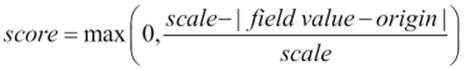
In the preceding example, linear is the name of the decay function. The value will decay linearly when using it. The other possible values are gauss and exp. We've chosen the linear decay function because it sets the score to 0 when the field value exceeds the given origin value twice. This is useful when you want to lower the value of the documents that are too far away.
We have presented the relevant equations to give you an idea of how the score is calculated by the given function. The linear decay function calculates the score of the document using the following equation:
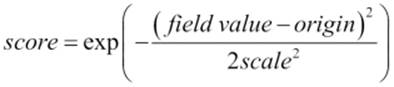
The gauss decay function calculates the score of the document using the following equation:
The exp decay function calculates the score of the document using the following equation:
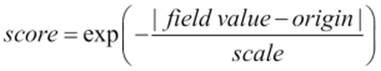
Of course, you don't need to calculate your document scores using pen and paper every time, but you may need it once in a while, and these equations may come in handy at such times.
Now, let's discuss the rest of the query structure. The field we want to use for score calculation is named point. If the document doesn't have a value in the defined field, it will be given a value of 1 at the time of calculation.
In addition to that, we've provided additional parameters. The origin and scale parameters are required. The origin parameter is the central point from which the calculation will be performed and scale is the rate of decay. By default, the offset parameter is set to 0; if defined, the decay function will only compute a score for documents with values greater than the value of this parameter. The decay parameter tells Elasticsearch how much the score should be lowered; it is set to 0.5 by default. In our case, we've said that at the distance of 1 kilometer, the score should be reduced by 20 percent (0.2).
Note
We expect the number of function scores available to be extended with newer versions of Elasticsearch and we suggest following the official documentation and the page dedicated to the function_score query available athttp://www.elasticsearch.org/guide/en/elasticsearch/reference/current/query-dsl-function-score-query.html.
Deprecated queries
After an introduction to the function_score query, the custom_boost, custom_score, and custom_filters_score queries were deprecated. The following section shows how to achieve the same results as we did with the mentioned queries by using the function_score query. This section is provided as a reference for those who want to migrate from older versions of Elasticsearch and alter their queries to remove the deprecated ones.
Replacing the custom_boost_factor query
Let's assume that we have the following custom_boost_factor query:
{
"query" : {
"custom_boost_factor" : {
"query": {
"term" : { "author" : "heller" }
},
"boost_factor": 5.0
}
}
}
To replace the preceding query with the function_score query, we would have to use the following query:
{
"query" : {
"function_score" : {
"query": {
"term" : { "author" : "heller" }
},
"functions" : [
{ "boost_factor": 5.0 }
]
}
}
}
Replacing the custom_score query
The second type of deprecated queries is the constant_score query. Let's assume that we have the following custom_score query:
{
"query" : {
"custom_score" : {
"query" : { "match_all" : {} },
"script" : "_source.copies * 0.5"
}
}
}
If we want to replace it with the function_score query, it will look as follows:
{
"query" : {
"function_score" : {
"boost_mode" : "replace",
"query" : { "match_all" : {} },
"functions" : [
{
"script_score" : {
"script" : "_source.copies * 0.5"
}
}
]
}
}
}
Replacing the custom_filters_score query
The last query replacement we will discuss is the custom_filters_score query. Let's assume we have the following query:
{
"query" : {
"custom_filters_score" : {
"query" : { "match_all" : {} },
"filters" : [
{
"filter" : { "term" : { "available" : true }},
"boost" : 10
}
],
"score_mode" : "first"
}
}
}
If we want to replace it with the function_score query, it will look as follows:
{
"query" : {
"function_score" : {
"query" : { "match_all" : {} },
"functions" : [
{
"filter" : { "term" : { "available" : true }},
"boost_factor" : 10
}
],
"score_mode" : "first"
}
}
}
When does index-time boosting make sense?
In the previous section, we discussed boosting queries. This type of boosting is very handy and powerful and fulfills its role in most situations. However, there is one case when the more convenient way is to use index-time boosting. This is the situation when we know which documents are important during the index phase. We gain a boost that is independent from a query at the cost of reindexing (we need to reindex the document when the boost value is changed). In addition to that, the performance is slightly better because some parts needed in the boosting process are already calculated at index time. Elasticsearch stores information about the boost as a part of normalization information. This is important because if we set omit_norms to true, we can't use index-time boosting.
Defining field boosting in input data
Let's look at the typical document definition, which looks as follows:
{
"title" : "The Complete Sherlock Holmes",
"author" : "Arthur Conan Doyle",
"year" : 1936
}
If we want to boost the author field for this particular document, the structure should be slightly changed and the document should look as follows:
{
"title" : "The Complete Sherlock Holmes",
"author" : {
"_value" : "Arthur Conan Doyle",
"_boost" : 10.0,
},
"year": 1936
}
And that's all. After indexing the preceding document, we will let Elasticsearch know that the importance of the author field is greater than the rest of the fields.
Note
In older versions of Elasticsearch, setting document-wide boost was possible. However, starting with 4.0, Lucene doesn't support whole document boosting and Elasticsearch emulated it by boosting all the fields in the document. In Elasticsearch 1.0, the document boost was deprecated and we decided not to write about it, because it will be removed in the future.
Defining boosting in mapping
It is worth mentioning that it is possible to directly define the field's boost in our mappings. The following example illustrates this:
{
"mappings" : {
"book" : {
"properties" : {
"title" : { "type" : "string" },
"author" : { "type" : "string", "boost" : 10.0 }
}
}
}
}
Thanks to the preceding boost, all queries will favor values found in the field named author. This also applies to queries using the _all field.
Words with the same meaning
You may have heard about synonyms—words that have the same or similar meaning. Sometimes, you will want to have some words match when one of those words is entered into the search box. Let's recall our sample data from The example data section ofChapter 3, Searching Your Data; there was a book called Crime and Punishment. What if we want that book to be matched not only when the words crime or punishment are used, but also when using words like criminality and abuse. To perform this, we will use synonyms.
The synonym filter
In order to use the synonym filter, we need to define our own analyzer. Our analyzer will be called synonym and will use the whitespace tokenizer and a single filter called synonym. Our filter's type property needs to be set to synonym, which tells Elasticsearch that this filter is a synonym filter. In addition to that, we want to ignore case so that upper- and lowercase synonyms will be treated equally (set the ignore_case property to true). To define our custom synonym analyzer that uses a synonym filter, we need to have the following mappings:
{
"index" : {
"analysis" : {
"analyzer" : {
"synonym" : {
"tokenizer" : "whitespace",
"filter" : [
"synonym"
]
}
},
"filter" : {
"synonym" : {
"type" : "synonym",
"ignore_case" : true,
"synonyms" : [
"crime => criminality"
]
}
}
}
}
}
Synonyms in the mappings
In the preceding definition, we specified the synonym rule in the mappings we send to Elasticsearch. In order to do that, we need to add the synonyms property, which is an array of synonym rules. For example, the following part of the mappings definition defines a single synonym rule:
"synonyms" : [
"crime => criminality"
]
We will discuss how to define the synonym rules in just a second.
Synonyms stored in the filesystem
Elasticsearch also allows us to use file-based synonyms. To use a file, we need to specify the synonyms_path property instead of the synonyms property. The synonyms_path property should be set to the name of the file that holds the synonym's definition and the specified file path should be relative to the Elasticsearch config directory. So, if we store our synonyms in the synonyms.txt file and save that file in the config directory, in order to use it, we should set synonyms_path to the value of synonyms.txt.
For example, the following shows how the synonym filter (the one from the preceding mappings) will be if we want to use the synonyms stored in a file:
"filter" : {
"synonym" : {
"type" : "synonym",
"synonyms_path" : "synonyms.txt"
}
}
Defining synonym rules
Till now, we discussed what we have to do in order to use synonym expansions in Elasticsearch. Now, let's see what formats of synonyms are allowed.
Using Apache Solr synonyms
The most common synonym structure in the Apache Lucene world is probably the one used by Apache Solr—the search engine built on top of Lucene, just like Elasticsearch. This is the default way to handle synonyms in Elasticsearch, and the possibilities of defining a new synonym are discussed in the following sections.
Explicit synonyms
A simple mapping allows us to map a list of words into other words. So, in our case, if we want the word criminality to be mapped to crime and the word abuse to be mapped to punishment, we need to define the following entries:
criminality => crime
abuse => punishment
Of course, a single word can be mapped into multiple words and multiple ones can be mapped into a single word, as follows:
star wars, wars => starwars
The preceding example means that star wars and wars will be changed to starwars by the synonym filter.
Equivalent synonyms
In addition to explicit mapping, Elasticsearch allows us to use equivalent synonyms. For example, the following definition will make all the words exchangeable so that you can use any of them to match a document that has one of them in its contents:
star, wars, star wars, starwars
Expanding synonyms
A synonym filter allows us to use one additional property when it comes to the synonyms of the Apache Solr format—the expand property. When the expand property is set to true (by default, it is set to false), all synonyms will be expanded by Elasticsearch to all equivalent forms. For example, let's say we have the following filter configuration:
"filter" : {
"synonym" : {
"type" : "synonym",
"expand": false,
"synonyms" : [
"one, two, three"
]
}
}
Elasticsearch will map the preceding synonym definition to the following:
one, two, thee => one
This means that the words one, two, and three will be changed to one. However, if we set the expand property to true, the same synonym definition will be interpreted in the following way:
one, two, three => one, two, three
This basically means that each of the words from the left-hand side of the definition will be expanded to all the words on the right-hand side.
Using WordNet synonyms
If we want to use WordNet-structured synonyms (to learn more about WordNet, visit http://wordnet.princeton.edu/), we need to provide an additional property for our synonym filter. The property name is format and we should set its value to wordnet in order for Elasticsearch to understand that format.
Query- or index-time synonym expansion
As with all analyzers, one can wonder when we should use our synonym filter—during indexing, during querying, or maybe during indexing and querying. Of course, it depends on your needs; however, remember that using index-time synonyms requires data reindexing after each synonym change. That's because they need to be reapplied to all the documents. If we use only query-time synonyms, we can update the synonym lists and have them applied during the query.
Understanding the explain information
Compared to databases, using systems that are capable of performing full-text search can often be anything other than obvious. We can search in many fields simultaneously, and the data in the index can vary from the ones provided as the values of the document fields (because of the analysis process, synonyms, abbreviations, and others). It's even worse; by default, search engines sort data by relevance—a number that indicates how similar the document is to the query. The key here is how similar. As we already discussed, scoring takes many factors into account: how many searched words were found in the document, how frequent the word was, how many terms were present in the field, and so on. This seems complicated, and finding out why a document was found and why another document is better is not easy. Fortunately, Elasticsearch has some tools that can answer these questions, and we will look at them now.
Understanding field analysis
One of the common questions asked is why a given document was not found. In many cases, the problem lies in the mappings definition and the analysis process configuration. For debugging the analysis process, Elasticsearch provides a dedicated REST API endpoint, _analyze.
Let's start with looking at the information returned by Elasticsearch for the default analyzer. To do that, we will run the following command:
curl -XGET 'localhost:9200/_analyze?pretty' -d 'Crime and Punishment'
In response, we will get the following data:
{
"tokens" : [ {
"token" : "crime",
"start_offset" : 0,
"end_offset" : 5,
"type" : "<ALPHANUM>",
"position" : 1
}, {
"token" : "punishment",
"start_offset" : 10,
"end_offset" : 20,
"type" : "<ALPHANUM>",
"position" : 3
} ]
}
As we can see, Elasticsearch divided the input phrase into two tokens. During processing, the and common word was omitted (because it belongs to the stop words list) and the other words were turned into lowercase. This shows us exactly what would be happening during the analysis process. We can also provide the name of the analyzer, for example, we can change the preceding command as follows:
curl -XGET 'localhost:9200/_analyze?analyzer=standard&pretty' -d 'Crime and Punishment'
The preceding command will allow us to check how the standard analyzer analyzes the data (it will be a bit different from the response we've seen previously).
It is worth noting that there is another form of analysis API available—the one that allows us to provide tokenizers and filters. It is very handy when we want to experiment with the configuration before creating the target mappings. An example of such a call is as follows:
curl -XGET 'localhost:9200/library/_analyze?tokenizer=whitespace&filters=lowercase,kstem&pretty' -d 'John Smith'
In the preceding example, we used the analyzer, which was built with the whitespace tokenizer and two filters, lowercase and kstem.
As we can see, an analysis API can be very useful for tracking down the bugs in the mapping configuration. It is also very useful for when we want to solve problems with queries and search relevance. It can show us how our analyzers work, what terms they produce, and what the attributes of those terms are. With such information, analyzing query problems will be easier to track down.
Explaining the query
In addition to looking at what happened during analysis, Elasticsearch allows us to explain how the score was calculated for a particular query and document. Let's look at the following example:
curl -XGET 'localhost:9200/library/book/1/_explain?pretty&q=quiet'
In the preceding call, we provided a specific document and a query to run. Using the _explain endpoint, we ask Elasticsearch for an explanation on how the document was matched by Elasticsearch (or not matched). For example, should the preceding document be found by the provided query? If it is, Elasticsearch will provide information on why the document was matched, along with details about how its score was calculated.
The result returned by Elasticsearch for the preceding command is as follows:
{
"_index" : "library",
"_type" : "book",
"_id" : "1",
"matched" : true,
"explanation" : {
"value" : 0.057534903,
"description" : "weight(_all:quiet in 0) [PerFieldSimilarity], result of:",
"details" : [ {
"value" : 0.057534903,
"description" : "fieldWeight in 0, product of:",
"details" : [ {
"value" : 1.0,
"description" : "tf(freq=1.0), with freq of:",
"details" : [ {
"value" : 1.0,
"description" : "termFreq=1.0"
} ]
}, {
"value" : 0.30685282,
"description" : "idf(docFreq=1, maxDocs=1)"
}, {
"value" : 0.1875,
"description" : "fieldNorm(doc=0)"
} ]
} ]
}
}
Looks complicated, and, well, it is complicated! What's even worse is that this is only a simple query! Elasticsearch, and more specifically, the Lucene library, shows the internal information about the scoring process. We will only scratch the surface and will explain the most important things about the preceding response.
The most important part is the total score calculated for a document (the value property of the explanation object). If it is equal to 0, the document didn't match the given query. Another important element is the description section that tells us which similarity was used. In our example, we were looking for the quiet term. It was found in the _all field. It is obvious because we searched in the default field, which is _all (you should remember this field from the Extending your index structure with additional internal informationsection in Chapter 2, Indexing Your Data).
The details section provides us with information about components and where we should seek explanation about why our document matches the query. When it comes to scoring, we have a single object present—a single component that was responsible for document score calculation. The value property is the score calculated by this component, and again we see the description and details section. As you can see in the description field, the final score is the product of (fieldWeight in 0, product of) all the scores calculated by each element in the inner details array (1.0 * 0.30685282 * 0.1875).
In the inner details array, we can see three objects. The first one shows information about the term frequency in the given field (which was 1 in our case). This means that the field contained only a single occurrence of the searched term. The second object shows the inverse document frequency. Note the maxDocs property, which is equal to 1. This means that only one document was found with the specified term. The third object is responsible for the field norm for that field.
Note that the preceding response will be different for each query. What's more, the more complicated the query will be, the more complicated the returned information will be.
Summary
In this chapter, we learned how Apache Lucene scoring works internally. We've also seen how to use the scripting capabilities of Elasticsearch and how to index and search documents in different languages. We've used different queries to alter the score of our documents and modify it so it fits our use case. We've learned about index-time boosting, what synonyms are, and how they can help us. Finally, we've seen how to check why a particular document was a part of the result set and how its score was calculated.
In the next chapter, we'll go beyond full-text searching. We'll see what aggregations are and how we can use them to analyze our data. We'll also see faceting, which also allows us to aggregate our data and bring meaning to it. We'll use suggesters to implement spellchecking and autocomplete, and we'll use prospective search to find out which documents match particular queries. We'll index binary files and use geospatial capabilities to search our data with the use of geographical data. Finally, we'll use the scroll API to efficiently fetch a large number of results and we'll see how to make Elasticsearch use a list of terms (a list that is loaded automatically) in a query.
All materials on the site are licensed Creative Commons Attribution-Sharealike 3.0 Unported CC BY-SA 3.0 & GNU Free Documentation License (GFDL)
If you are the copyright holder of any material contained on our site and intend to remove it, please contact our site administrator for approval.
© 2016-2026 All site design rights belong to S.Y.A.