Elasticsearch Server, Second Edition (2014)
Chapter 6. Beyond Full-text Searching
In the previous chapter, we saw how Apache Lucene scoring works internally. We saw how to use the scripting capabilities of Elasticsearch and how to index and search documents in different languages. We learned how to use different queries in order to alter the score of our documents, and we used index-time boosting. We learned what synonyms are and finally, we saw how to check why a particular document was a part of the result set and how its score was calculated. By the end of this chapter, you will have learned the following topics:
· Using aggregations to aggregate our indexed data and calculate useful information from it
· Employing faceting to calculate different statistics from our data
· Implementing the spellchecking and autocomplete functionalities by using Elasticsearch suggesters
· Using prospective search to match documents against queries
· Indexing binary files
· Indexing and searching geographical data
· Efficiently fetching large datasets
· Automatically loading terms and using them in our query
Aggregations
Apart from the improvements and new features that Elasticsearch 1.0 brings, it also includes a highly anticipated framework, which moves Elasticsearch to a new position—a full-featured analysis engine. Now, you can use Elasticsearch as a key part of various systems that process massive volumes of data, allow you to extract conclusions, and visualize that data in a human-readable way. Let's see how this functionality works and what we can achieve by using it.
General query structure
To use aggregation, we need to add an additional section in our query. In general, our queries with aggregations will look like the following code snippet:
{
"query": { … },
"aggs" : { … }
}
In the aggs property (you can use aggregations if you want; aggs is just an abbreviation), you can define any number of aggregations. One thing to remember though is that the key defines the name of the aggregation (you will need it to distinguish particular aggregations in the server response). Let's take our library index and create the first query that will use aggregations. A command to send such a query is as follows:
curl 'localhost:9200/_search?search_type=count&pretty' -d '{
"aggs": {
"years": {
"stats": {
"field": "year"
}
},
"words": {
"terms": {
"field": "copies"
}
}
}
}'
This query defines two aggregations. The aggregation named years shows the statistics for the year field. The words aggregation contains information about the terms used in a given field.
Note
In our examples, we assumed that we do aggregation in addition to searching. If we don't need the documents that are found, a better idea is to use the search_type=count parameter. This omits some unnecessary work and is more efficient. In such a case, the endpoint should be /library/_search?search_type=count. You can read more about the search types in the Understanding the querying process section of Chapter 3, Searching Your Data.
Now let's look at the response returned by Elasticsearch for the preceding query:
{
"took": 2,
"timed_out": false,
"_shards": {
"total": 5,
"successful": 5,
"failed": 0
},
"hits": {
"total": 4,
"max_score": 0,
"hits": []
},
"aggregations": {
"words": {
"buckets": [
{
"key": 0,
"doc_count": 2
},
{
"key": 1,
"doc_count": 1
},
{
"key": 6,
"doc_count": 1
}
]
},
"years": {
"count": 4,
"min": 1886,
"max": 1961,
"avg": 1928,
"sum": 7712
}
}
}
As you can see, both the aggregations (years and words) were returned. The first aggregation we defined in our query (years) returned general statistics for the given field, which was gathered across all the documents that matched our query. The second aggregation (words) is a bit different. It created several sets called buckets that are calculated on the returned documents, and each of the aggregated values is present within one of these sets. As you can see, there are multiple aggregation types available and they return different results. We will see the differences later in this section.
Available aggregations
After the previous example, you shouldn't be surprised that aggregations are divided into groups. Currently, there are two groups—metric aggregations and bucketing aggregations.
Metric aggregations
Metric aggregations take an input document set and generate at least a single statistic. As you will see, these aggregations are mostly self-explanatory.
Min, max, sum, and avg aggregations
Usage of the min, max, sum, and avg aggregations is very similar. For the given field, they return a minimum value, a maximum value, a sum of all the values, and an average value, respectively. Any numeric field can be used as a source for these values. For example, to calculate the minimum value for the year field, we will construct the following aggregation:
{
"aggs": {
"min_year": {
"min": {
"field": "year"
}
}
}
}
The returned result will be similar to the following one:
"min_year": {
"value": 1886
}
Using scripts
The input values can also be generated by a script. For example, if we want to find a minimum value from all the values in the year field, but we also want to subtract 1000 from these values, we will send an aggregation similar to the following one:
{
"aggs": {
"min_year": {
"min": {
"script": "doc['year'].value - 1000"
}
}
}
In this case, the value that the aggregations will use is the original year field value reduced by 1000. The other notation that we can use to achieve the same response is to provide the field name and the script property, as follows:
{
"aggs": {
"min_year": {
"min": {
"field": "year",
"script": "_value - 1000"
}
}
}
}
The field name is given outside the script. If we like, we can be even more verbose, as follows:
{
"aggs": {
"min_year": {
"min": {
"field": "year",
"script": "_value - mod",
"params": {
"mod" : 1000
}
}
}
}
}
As you can see, we've added the params section with additional parameters. You can read more about scripts in the Scripting capabilities of Elasticsearch section of Chapter 5, Make Your Search Better.
The value_count aggregation
The value_count aggregation is similar to the ones we described previously, but the input field doesn't have to be numeric. An example of this aggregation is as follows:
{
"aggs": {
"number_of_items": {
"value_count": {
"field": "characters"
}
}
}
}
Let's stop here for a moment. It is a good opportunity to look at which values are counted by Elasticsearch aggregation in this case. If you run the preceding query on your index with books (the library index), the response will be something as follows:
"number_of_items": {
"value": 31
}
Elasticsearch counted all the tokens from the characters field across all the documents. This number makes sense when we keep in mind that, for example, our Sofia Semyonovna Marmeladova term will become sofia, semyonovna, and marmeladova after analysis. In most of the cases, such a behavior is not what we are aiming at. For such cases, we should use a not-analyzed version of the characters field.
The stats and extended_stats aggregations
The stats and extended_stats aggregations can be treated as aggregations that return all the previously described aggregations but within a single aggregation object. For example, if we want to calculate statistics for the year field, we can use the following code:
{
"aggs": {
"stats_year": {
"stats": {
"field": "year"
}
}
}
}
The relevant part of the results returned by Elasticsearch will be as follows:
"stats_year": {
"count": 4,
"min": 1886,
"max": 1961,
"avg": 1928,
"sum": 7712
}
Of course, the extended_stats aggregation returns statistics that are even more extended. Let's look at the following query:
{
"aggs": {
"stats_year": {
"extended_stats": {
"field": "year"
}
}
}
}
In the returned response, we will see the following output:
"stats_year": {
"count": 4,
"min": 1886,
"max": 1961,
"avg": 1928,
"sum": 7712,
"sum_of_squares": 14871654,
"variance": 729.5,
"std_deviation": 27.00925767213901
}
As you can see, in addition to the already known values, we also got the sum of squares, variance, and the standard deviation statistics.
Bucketing
Bucketing aggregations return many subsets and qualify the input data to a particular subset called bucket. You can think of the bucketing aggregations as something similar to the former faceting functionality described in the Faceting section. However, the aggregations are more powerful and just easier to use. Let's go through the available bucketing aggregations.
The terms aggregation
The terms aggregation returns a single bucket for each term available in a field. This allows you to generate the statistics of the field value occurrences. For example, the following are the questions that can be answered by using this aggregation:
· How many books were published each year?
· How many books were available for borrowing?
· How many copies of the books do we have the most?
To get the answer for the last question, we can send the following query:
{
"aggs": {
"availability": {
"terms": {
"field": "copies"
}
}
}
}
The response returned by Elasticsearch for our library index is as follows:
"availability": {
"buckets": [
{
"key": 0,
"doc_count": 2
},
{
"key": 1,
"doc_count": 1
},
{
"key": 6,
"doc_count": 1
}
]
}
We see that we have two books without copies available (bucket with the key property equal to 0), one book with one copy (bucket with the key property equal to 1), and a single book with six copies (bucket with the key property equal to 6). By default, Elasticsearch returns the buckets sorted by the value of the doc_count property in descending order. We can change this by adding the order attribute. For example, to sort our aggregations by using the key property values, we will send the following query:
{
"aggs": {
"availability": {
"terms": {
"field": "copies",
"size": 40,
"order": { "_term": "asc" }
}
}
}
}
We can sort in incremental order (asc) or in decremental order (desc). In our example, we sorted the values by using their key properties (_term). The other option available is _count, which tells Elasticsearch to sort by the doc_count property.
In the preceding example, we also added the size attribute. As you can guess, it defines how many buckets should be returned at the maximum.
Note
You should remember that when the field is analyzed, you will get buckets from the analyzed terms as shown in the example with the value count. This probably is not what you want. The answer to such a problem is just to add an additional, not-analyzed version of your field to the index and to use it for the aggregation calculation.
The range aggregation
In the range aggregation, buckets are created using defined ranges. For example, if we want to check how many books were published in the given period of time, we can create the following query:
{
"aggs": {
"years": {
"range": {
"field": "year",
"ranges": [
{ "to" : 1850 },
{ "from": 1851, "to": 1900 },
{ "from": 1901, "to": 1950 },
{ "from": 1951, "to": 2000 },
{ "from": 2001 }
]
}
}
}
}
For the data in the library index, the response should look like the following output:
"years": {
"buckets": [
{
"to": 1850,
"doc_count": 0
},
{
"from": 1851,
"to": 1900,
"doc_count": 1
},
{
"from": 1901,
"to": 1950,
"doc_count": 2
},
{
"from": 1951,
"to": 2000,
"doc_count": 1
},
{
"from": 2001,
"doc_count": 0
}
]
}
For example, from the preceding output, we know that between 1901 and 1950, we released two books.
If you create the user interface, it is possible to automatically generate a label for every bucket. Turning on this feature is simple—we just need to add the keyed attribute and set it to true, just like in the following example:
{
"aggs": {
"years": {
"range": {
"field": "year",
"keyed": true,
"ranges": [
{ "to" : 1850 },
{ "from": 1851, "to": 1900 },
{ "from": 1901, "to": 1950 },
{ "from": 1951, "to": 2000 },
{ "from": 2001 }
]
}
}
}
}
The highlighted part in the preceding code causes the results to contain labels, just as we can see in the following response returned by Elasticsearch:
"years": {
"buckets": {
"*-1850.0": {
"to": 1850,
"doc_count": 0
},
"1851.0-1900.0": {
"from": 1851,
"to": 1900,
"doc_count": 1
},
"1901.0-1950.0": {
"from": 1901,
"to": 1950,
"doc_count": 2
},
"1951.0-2000.0": {
"from": 1951,
"to": 2000,
"doc_count": 1
},
"2001.0-*": {
"from": 2001,
"doc_count": 0
}
}
}
As you probably noticed, the structure is slightly changed—now, the buckets field is not a table but a map where the key is generated from the range. This works, but it is not so pretty. For our case, giving a name for every bucket will be more useful. Fortunately, it is possible and we can do this by adding the key attribute for every range and setting its value to the desired name. Consider the following example:
{
"aggs": {
"years": {
"range": {
"field": "year",
"keyed": true,
"ranges": [
{ "key": "Before 18th century", "to": 1799 },
{ "key": "18th century", "from": 1800, "to": 1899 },
{ "key": "19th century", "from": 1900, "to": 1999 },
{ "key": "After 19th century", "from": 2000 }
]
}
}
}
}
Note
It is important and quite useful that ranges need not be disjoint. In such cases, Elasticsearch will properly count the document for multiple buckets.
The date_range aggregation
The date_range aggregation is similar to the previously discussed range aggregation, but it is designed for the fields that use date types. Although the library index documents have the years mentioned in them, the field is a number and not a date. To test this, let's imagine that we want to extend our library index to support newspapers. To do this, we will create a new index called library2 by using the following command:
curl -XPOST localhost:9200/_bulk --data-binary '{ "index": {"_index": "library2", "_type": "book", "_id": "1"}}
{ "title": "Fishing news", "published": "2010/12/03 10:00:00", "copies": 3, "available": true }
{ "index": {"_index": "library2", "_type": "book", "_id": "2"}}
{ "title": "Knitting magazine", "published": "2010/11/07 11:32:00", "copies": 1, "available": true }
{ "index": {"_index": "library2", "_type": "book", "_id": "3"}}
{ "title": "The guardian", "published": "2009/07/13 04:33:00", "copies": 0, "available": false }
{ "index": {"_index": "library2", "_type": "book", "_id": "4"}}
{ "title": "Hadoop World", "published": "2012/01/01 04:00:00", "copies": 6, "available": true }
'
In the library2 index, we leave the mapping for Elasticsearch discovery mechanisms—this is sufficient in this case. Let's start with the first query using the date_range aggregation, which is as follows:
{
"aggs": {
"years": {
"date_range": {
"field": "published",
"ranges": [
{ "to" : "2009/12/31" },
{ "from": "2010/01/01", "to": "2010/12/31" },
{ "from": "2011/01/01" }
]
}
}
}
}
Comparing with the ordinary range aggregation, the only thing that changed is the aggregation type (date_range). The dates can be passed in a string format recognized by Elasticsearch (refer to Chapter 2, Indexing Your Data, for more information) or as a number value—the number of milliseconds since 1970-01-01). The response returned by Elasticsearch is as follows:
"years": {
"buckets": [
{
"to": 1262217600000,
"to_as_string": "2009/12/31 00:00:00",
"doc_count": 1
},
{
"from": 1262304000000,
"from_as_string": "2010/01/01 00:00:00",
"to": 1293753600000,
"to_as_string": "2010/12/31 00:00:00",
"doc_count": 2
},
{
"from": 1293840000000,
"from_as_string": "2011/01/01 00:00:00",
"doc_count": 1
}
]
}
The only difference in the preceding response compared to the response given by the range aggregation is that the information about the range boundaries is split into two attributes. The attributes named from or to present the number of milliseconds from 1970-01-01. The properties from_as_string and to_as_string present the date in a human-readable form. Of course, the keyed and key attributes in the definition of the date_range aggregation work as already described.
Elasticsearch also allows us to define the format of the presented dates by using the format attribute. In our example, we presented the dates with year resolution, so mentioning the day and time were unnecessary. If we want to show month names, we can send a query like the following:
{
"aggs": {
"years": {
"date_range": {
"field": "published",
"format": "MMMM YYYY",
"ranges": [
{ "to" : "2009/12/31" },
{ "from": "2010/01/01", "to": "2010/12/31" },
{ "from": "2011/01/01" }
]
}
}
}
}
One of the returned ranges looks as follows:
{
"from": 1262304000000,
"from_as_string": "January 2010",
"to": 1293753600000,
"to_as_string": "December 2010",
"doc_count": 2
}
Looks better, doesn't it?
Note
The available formats that we can use in the format parameter are defined in the Joda Time library. The full list is available at http://joda-time.sourceforge.net/apidocs/org/joda/time/format/DateTimeFormat.html.
There is one more thing about the date_range aggregation. Sometimes, we may want to build an aggregation that can change with time. For example, we want to see how many newspapers were published in every quarter. This is possible without modifying our query. To do this, consider the following example:
{
"aggs": {
"years": {
"date_range": {
"field": "published",
"format": "dd-MM-YYYY",
"ranges": [
{ "to" : "now-9M/M" },
{ "to" : "now-9M" },
{ "from": "now-6M/M", "to": "now-9M/M" },
{ "from": "now-3M/M" }
]
}
}
}
}
The keys are the expressions such as now-9M. Elasticsearch does the math and generates the appropriate value. You can use y (year), M (month), w (week), d (day), h (hour), m (minute), and s (second). For example, the expression now+3d means three days from now. The /M expression in our example takes only the dates that have been rounded to months. Thanks to such notations, we count only full months. The second advantage is that the calculated date is more cache-friendly—without rounding off, the date changes every millisecond, which causes every cache based on the range to become irrelevant.
IPv4 range aggregation
The last form of the range aggregation is aggregation based on Internet addresses. It works on the fields defined with the ip type and allows you to define ranges given by the IP range in the CIDR notation (http://en.wikipedia.org/wiki/Classless_Inter-Domain_Routing). An example of the ip_range aggregation looks as follows:
{
"aggs": {
"access": {
"ip_range": {
"field": "ip",
"ranges": [
{ "from": "192.168.0.1", "to": "192.168.0.254" },
{ "mask": "192.168.1.0/24" }
]
}
}
}
}
The response to the preceding query can be as follows:
"access": {
"buckets": [
{
"from": 3232235521,
"from_as_string": "192.168.0.1",
"to": 3232235774,
"to_as_string": "192.168.0.254",
"doc_count": 0
},
{
"key": "192.168.1.0/24",
"from": 3232235776,
"from_as_string": "192.168.1.0",
"to": 3232236032,
"to_as_string": "192.168.2.0",
"doc_count": 4
}
]
}
Again, the keyed and key attributes here work just like in the range aggregation.
The missing aggregation
Let's get back to our library index and check how many entries have no original title defined (the otitle field). To do this, we will use the missing aggregation, which will be a good friend in this case. An example query will look as follows:
{
"aggs": {
"missing_original_title": {
"missing": {
"field": "otitle"
}
}
}
}
The relevant response part looks as follows:
"missing_original_title": {
"doc_count": 2
}
We have two documents without the otitle field.
Note
The missing aggregation is aware of the fact that the mapping definition may have null_value defined and will need to count the documents independently from this definition.
Nested aggregation
In the Using nested objects section of Chapter 4, Extending Your Index Structure, we learned about nested documents. Let's use this data to look into the next type of aggregation—the nested aggregation. Let's create the simplest working query, which will look as follows:
{
"aggs": {
"variations": {
"nested": {
"path": "variation"
}
}
}
}
The preceding query is similar in structure to any other aggregation. It contains a single parameter—path, which points to the nested document. In the response, we get a number, as shown in the following output:
"variations": {
"doc_count": 2
}
The preceding response means that we have two nested documents in the index with the provided variation type.
The histogram aggregation
The histogram aggregation is an aggregation that defines the buckets. The simplest form of a query that uses this aggregation looks as follows:
{
"aggs": {
"years": {
"histogram": {
"field" : "year",
"interval": 100
}
}
}
}
The new piece of information here is interval, which defines the length of every range that will be used to create a bucket. Because of this, in our example, buckets will be created for periods of 100 years. The aggregation part of the response to the preceding query that was sent to our library index is as follows:
"years": {
"buckets": [
{
"key": 1800,
"doc_count": 1
},
{
"key": 1900,
"doc_count": 3
}
]
}
As in the range aggregation, histogram also allows us to use the keyed property. The other available option is min_doc_count, which allows us to control what is the minimal number of documents required to create a bucket. If we set the min_doc_count property to zero, Elasticsearch will also include the buckets with the document count of 0.
The date_histogram aggregation
As the date_range aggregation is a specialized form of the range aggregation, the date_histogram aggregation is an extension of the histogram aggregation that works on dates. So, again we will use our index with newspapers (it was called library2). An example of the query that uses the date_histogram aggregation looks as follows:
{
"aggs": {
"years": {
"date_histogram": {
"field" : "published",
"format" : "yyyy-MM-dd HH:mm",
"interval": "10d"
}
}
}
}
We can spot one important difference to the interval property. It is now a string describing the time interval, which in our case is ten days. Of course, we can set it to anything we want—it uses the same suffixes that we discussed when talking about the formats in the date_range aggregation. It is worth mentioning that the number can be a float value; for example, 1.5m, which means every one and a half minutes. The format attribute is the same as in the date_range aggregation—thanks to this, Elasticsearch can add a human-readable date according to the defined format. Of course, the format attribute is not required, but it is useful.
In addition to this, similar to the other range aggregations, the keyed and min_doc_count attributes still work.
Time zones
Elasticsearch stores all the dates in the UTC time zone. You can define the time zone, which should be used for display purposes. There are two ways for date conversion; Elasticsearch can convert a date before assigning an element to the appropriate bucket or after the assignment is done. This leads to the situation where an element may be assigned to various buckets depending on the chosen way and the definition of the bucket. We have two attributes that define this pre_zone and post_zone. Also, there is atime_zone attribute that basically sets the pre_zone attribute value. There are three notations to set these attributes, which are as follows:
· We can set the hours offset; for example: pre_zone:-4 or time_zone:5
· We can use the time format; for example: pre_zone:"-4:30"
· We can use name of the time zone; for example: time_zone:"Europe/Warsaw"
Note
Look at http://joda-time.sourceforge.net/timezones.html to see the available time zones.
The geo_distance aggregation
The next two aggregations are connected with maps and spatial search. We will talk about the geo types and queries later in this chapter, so feel free to skip these two topics now and return to them later.
Look at the following query:
{
"aggs": {
"neighborhood": {
"geo_distance": {
"field": "location",
"origin": [-0.1275, 51.507222],
"ranges": [
{ "to": 1200 },
{ "from": 1201 }
]
}
}
}
}
You can see that this query is similar to the range aggregation. The preceding aggregation will calculate the number of cities that fall into two buckets: one bucket of cities within 1200 km, and the second bucket of cities further than 1200 km from the origin (in this case, the origin is London). The aggregation section of the response returned by Elasticsearch looks similar to the following:
"neighborhood": {
"buckets": [
{
"key": "*-1200.0",
"from": 0,
"to": 1200,
"doc_count": 1
},
{
"key": "1201.0-*",
"from": 1201,
"doc_count": 4
}
]
}
Of course, the keyed and key attributes work in the geo_distance aggregation as well.
Now, let's modify the preceding query to show the other possibilities of the geo_distance aggregation as follows:
{
"aggs": {
"neighborhood": {
"geo_distance": {
"field": "location",
"origin": { "lon": -0.1275, "lat": 51.507222},
"unit": "m",
"distance_type" : "plane",
"ranges": [
{ "to": 1200 },
{ "from": 1201 }
]
}
}
}
}
We have highlighted three things in the preceding query. The first change is about how we define the point of origin. We can specify the location in various forms, which is described more precisely later in the chapter about geo type.
The second change is the unit attribute. The possible values are km (the default), mi, in, yd, m, cm, and mm that define the units of the numbers used in ranges (kilometers, miles, inches, yards, meters, centimeters, and millimeters, respectively).
The last attribute—distance_type—specifies how Elasticsearch calculates the distance. The possible values are (from the fastest but least accurate to the slowest but the most accurate) plane, sloppy_arc (the default), and arc.
The geohash_grid aggregation
Now you know how to aggregate based on the distance from a given point. The second option is to organize areas as a grid and assign every location to an appropriate cell. For this purpose, the ideal solution is Geohash (http://en.wikipedia.org/wiki/Geohash), which encodes the location into a string. The longer the string, the more accurate the description of a particular location will be. For example, one letter is sufficient to declare a box with about 5,000 x 5,000 km and five letters are enough to have the accuracy for about a 5 x 5 km square. Let's look at the following query:
{
"aggs": {
"neighborhood": {
"geohash_grid": {
"field": "location",
"precision": 5
}
}
}
}
We define the geohash_grid aggregation with buckets that have a precision of the mentioned square of 5 x 5 km (the precision attribute describes the number of letters used in the geohash string object). The table with resolutions versus the length of geohash can be found at http://www.elasticsearch.org/guide/en/elasticsearch/reference/master/search-aggregations-bucket-geohashgrid-aggregation.html.
Of course, more accuracy usually means more pressure on the system because of the number of buckets. By default, Elasticsearch will not generate more than 10,000 buckets. You can increase this parameter using the size attribute, but in fact, you should decrease it when possible.
Nesting aggregations
This is a powerful feature that allows us to build complex queries. Let's start expanding an example with the nested aggregation. In the example we used for nested aggregation, we only had the possibility of working with the nested documents. But, look at the following example to know what happens when we add the nested aggregation:
{
"aggs": {
"variations": {
"nested": {
"path": "variation"
},
"aggs": {
"sizes": {
"terms": {
"field": "variation.size"
}
}
}
}
}
}
As you can see, we've added another aggregation that was nested inside the top-level aggregation. The aggregation that has been nested is called sizes. The aggregation part of the result for the preceding query will look as follows:
"variations": {
"doc_count": 2,
"sizes": {
"buckets": [
{
"key": "XL",
"doc_count": 1
},
{
"key": "XXL",
"doc_count": 1
}
]
}
}
Perfect! Elasticsearch took the result from the parent aggregation and analyzed it using the terms aggregation. The aggregations can be nested even further—in theory, we can nest aggregations indefinitely. We can also have more aggregations on the same level.
Let's look at the following example:
{
"aggs": {
"years": {
"range": {
"field": "year",
"ranges": [
{ "to" : 1850 },
{ "from": 1851, "to": 1900 },
{ "from": 1901, "to": 1950 },
{ "from": 1951, "to": 2000 },
{ "from": 2001 }
]
},
"aggs": {
"statistics": {
"stats": {}
}
}
}
}
}
You will probably see that the preceding example is similar to the one we used when discussing the range aggregation. However, now we added an additional aggregation, which adds statistics to every bucket. The output for one of these buckets will look as follows:
{
"from": 1851,
"to": 1900,
"doc_count": 1,
"statistics": {
"count": 1,
"min": 1886,
"max": 1886,
"avg": 1886,
"sum": 1886
}
}
Note that in the stats aggregation, we omitted the information about the field that is used to calculate the statistics. Elasticsearch is smart enough to get this information from the context—in this case, the parent aggregation.
Bucket ordering and nested aggregations
Let's recall the example of the terms aggregation and ordering. We said that sorting is available on bucket keys or document count. This is only partially true. Elasticsearch can also use values from nested aggregations! Let's start with the following query example:
{
"aggs": {
"availability": {
"terms": {
"field": "copies",
"order": { "numbers.avg": "desc" }
},
"aggs": {
"numbers": { "stats" : {}}
}
}
}
}
In the preceding example, the order in the availability aggregation is based on the average value from the numbers aggregation. In this case, the numbers.avg notation is required because stats is a multivalued aggregation. If it was the sum aggregation, the name of the aggregation would be sufficient.
Global and subsets
All of our examples have one thing in common—the aggregations take into consideration the data from the whole index. The aggregation framework allows us to operate on the results filtered to the documents returned by the query or to do the opposite—ignore the query completely. You can also mix both the approaches. Let's analyze the following example:
{
"query": {
"filtered": {
"query": {
"match_all": {}
},
"filter": {
"term": {
"available": "true"
}
}
}
},
"aggs": {
"with_global": {
"global": {},
"aggs": {
"copies": {
"value_count": {
"field": "copies"
}
}
}
},
"without_global": {
"value_count": {
"field": "copies"
}
}
}
}
The first part is a query. In this case, we want to return all the books that are currently available. In the next part, we can see aggregations. They are named with_global and without_global. Both these aggregations are similar; they use the value_count aggregation on the copies field. The difference is that the with_global aggregation is nested in the global aggregation. This is something new—the global aggregation creates one bucket holding all the documents in the current search scope (this means all the indices and types we've used for searching), but ignores the defined queries. In other words, global aggregates all the documents, while without_global will make the aggregation work only on the documents returned by the query.
The aggregations section of the response to the preceding query looks as follows:
"aggregations": {
"without_global": {.
"value": 2
},
"with_global": {
"doc_count": 4,
"copies": {
"value": 4
}
}
}
In our index, we have two documents that match the query (books that are available now). The without_global aggregation did an aggregation on these documents, which gave a value equal to both the documents. The with_global aggregation ignores the search operation and operates on each document in the index, which means on all the four books.
Now, let's look at how to have a few aggregations and how one of these aggregations operates on a subset of a document. To do this, we can use a filter with aggregation, which will create one bucket containing the documents narrowed down for a given filter. Let's look at the following example:
{
"aggs": {
"with_filter": {
"filter": {
"term": {
"available": "true"
}
},
"aggs": {
"copies": {
"value_count": {
"field": "copies"
}
}
}
},
"without_filter": {
"value_count": {
"field": "copies"
}
}
}
}
We have no query to narrow down the number of documents that are passed to the aggregation, but we've included a filter that will narrow down the number of documents on which the aggregation will be calculated. The effect is the same as we've previously shown.
Inclusions and exclusions
The terms aggregation has one additional possibility of narrowing the number of aggregations—the include/exclude feature can be applied to string values. Let's look at the following query:
{
"aggs": {
"availability": {
"terms": {
"field": "characters",
"exclude": "al.*",
"include": "a.*"
}
}
}
}
The preceding query operates on a regular expression. It excludes all the terms starting with al from the aggregation calculation, but includes all the terms that start with a. The effect of such a query is that only the terms starting with the letter a will be counted, excluding the ones that have the l letter as the second letter in the word. The regular expressions are defined according to the JAVA API (http://docs.oracle.com/javase/7/docs/api/java/util/regex/Pattern.html) and Elasticsearch also allows you to define the flagsattribute as defined in this specification.
Faceting
Elasticsearch is a full-text search engine that aims to provide search results on the basis of our queries. However, sometimes we would like to get more—for example, we would like to get aggregated data that is calculated on the result set we get, such as the number of documents with a price between 100 and 200 dollars or the most common tags in the result documents. In the Aggregations section of this chapter, we talked about the aggregations framework. In addition to this, Elasticsearch provides a faceting module that is responsible for providing the functionality we've mentioned. In this chapter, we will discuss different faceting methods provided by Elasticsearch.
Note
Note that faceting offers a subset of functionality provided by the aggregation module. Because of this, Elasticsearch creators would like all the users to migrate from faceting to the mentioned aggregation module. Faceting is not deprecated and you can use it, but beware that sometime in the future, it may be removed from Elasticsearch.
The document structure
For the purpose of discussing faceting, we'll use a very simple index structure for our documents. It will contain the identifier of the document, document date, a multivalued field that can hold words describing our document (the tags field), and a field holding numeric information (the total field). Our mappings could look as follows:
{
"mappings" : {
"doc" : {
"properties" : {
"id" : { "type" : "long", "store" : "yes" },
"date" : { "type" : "date", "store" : "no" },
"tags" : { "type" : "string", "store" : "no", "index" : "not_analyzed" },
"total" : { "type" : "long", "store" : "no" }
}
}
}
}
Note
Keep in mind that when dealing with the string fields, you should avoid doing faceting on the analyzed fields. Such results may not be human-readable, especially when using stemming or any other heavy processing analyzers or filters.
Returned results
Before we get into how to run queries with faceting, let's take a look at what to expect from Elasticsearch in the result from a faceting request. In most of the cases, you'll only be interested in the data specific to the faceting type. However, in most faceting types, in addition to information specific to a given faceting type, you'll get the following information also:
· _type: This defines the faceting type used. This will be provided for each faceting type.
· missing: This defines the number of documents that didn't have enough data (for example, the missing field) to calculate faceting.
· total: This defines the number of tokens present in the facet calculation.
· other: This defines the number of facet values (for example, terms used in the terms faceting) that are not included in the returned counts.
In addition to this information, you'll get an array of calculated facets, such as count, for your terms, queries, or spatial distances. For example, the following code snippet shows how the usual faceting results look:
{
(...)
"facets" : {
"tags" : {
"_type" : "terms",
"missing" : 54715,
"total" : 151266,
"other" : 143140,
"terms" : [ {
"term" : "test",
"count" : 1119
}, {
"term" : "personal",
"count" : 1063
},
(...)
]
}
}
}
As you can see in the results, faceting was run against the tags field. We've got a total number of 151266 tokens processed by the faceting module and the 143140 tokens that were not included in the results. We also have 54715 documents that didn't have the value in the tags field. The test term appeared in 1119 documents, and the personal term appeared in 1063 documents. This is what you can expect from the faceting response.
Using queries for faceting calculations
Query is one of the simplest faceting types, which allows us to get the number of documents that match the query in the faceting results. The query itself can be expressed using the Elasticsearch query language, which we have already discussed. Of course, we can include multiple queries to get multiple counts in the faceting results. For example, faceting that will return the number of documents for a simple term query can look like the following code:
{
"query" : { "match_all" : {} },
"facets" : {
"my_query_facet" : {
"query" : {
"term" : { "tags" : "personal" }
}
}
}
}
As you can see, we've included the query type faceting with a simple term query. An example response for the preceding query could look as follows:
{
(...)
"facets" : {
"my_query_facet" : {
"_type" : "query",
"count" : 1081
}
}
}
As you can see in the response, we've got the faceting type and the count of the documents that matched the facet query, and of course, the main query results that we omitted in the preceding response.
Using filters for faceting calculations
In addition to using queries, Elasticsearch allows us to use filters for faceting calculations. It is very similar to query faceting, but instead of queries, filters are used. The filter itself can be expressed using the Elasticsearch query DSL, and of course, multiple filter facets can be used in a single request. For example, the faceting that will return the number of documents for a simple term filter can look as follows:
{
"query" : { "match_all" : {} },
"facets" : {
"my_filter_facet" : {
"filter" : {
"term" : { "tags" : "personal" }
}
}
}
}
As you can see, we've included the filter type faceting with a simple term filter. When talking about performance, the filter facets are faster than the query facets or the filter facets that wrap queries.
An example response for the preceding query will look as follows:
{
(...)
"facets" : {
"my_filter_facet" : {
"_type" : "filter",
"count" : 1081
}
}
}
As you can see in the response, we've got the faceting type and the count of the documents that matched the facet filter and the main query.
Terms faceting
Terms faceting allows us to specify a field that Elasticsearch will use and will return the top-most frequent terms. For example, if we want to calculate the most frequent terms for the tags field, we can run the following query:
{
"query" : { "match_all" : {} },
"facets" : {
"tags_facet_result" : {
"terms" : {
"field" : "tags"
}
}
}
}
The following faceting response will be returned by Elasticsearch for the preceding query:
{
(...)
"facets" : {
"tags_facet_result" : {
"_type" : "terms",
"missing" : 54716,
"total" : 151266,
"other" : 143140,
"terms" : [ {
"term" : "test",
"count" : 1119
}, {
"term" : "personal",
"count" : 1063
}, {
"term" : "feel",
"count" : 982
}, {
"term" : "hot",
"count" : 923
},
(...)
]
}
}
}
As you can see, our terms faceting results were returned in the tags_facet_result section and we've got the information that was already described.
There are a few additional parameters that we can use for the terms faceting, which are as follows:
· size: This parameter specifies how many of the top-most frequent terms should be returned at the maximum. The documents with the subsequent terms will be included in the count of the other field in the result.
· shard_size: This parameter specifies how many results per shard will be fetched by the node running the query. It allows you to increase the terms faceting accuracy in situations where the number of unique terms for a field is greater than the size parameter value. In general, the higher the size parameter, the more accurate are the results, but the more expensive is the calculation and more data is returned to the client. In order to avoid returning a long results list, we can set the shard_size value to a value higher than the value of the size parameter. This will tell Elasticsearch to use it to calculate the terms facets but still return a maximum of the size top terms. Please remember that the shard_size parameter cannot be set to a value lower than the size parameter.
· order: This parameter specifies the order of the facets. The possible values are count (by default this is ordered by frequency, starting from the most frequent), term (in ascending alphabetical order), reverse_count (ordered by frequency, starting from the less frequent), and reverse_term (in descending alphabetical order).
· all_terms: This parameter, when set to true, will return all the terms in the result, even those that don't match any of the documents. It can be demanding in terms of performance, especially on the fields with a large number of terms.
· exclude: This specifies the array of terms that should be excluded from the facet calculation.
· regex: This parameter specifies the regex expression that will control which terms should be included in the calculation.
· script: This parameter specifies the script that will be used to process the terms used in the facet calculation.
· fields: This parameter specifies the array that allows us to specify multiple fields for facet calculation (should be used instead of the field property). Elasticsearch will return aggregation across multiple fields. This property can also include a special value called _index. If such a value is present, the calculated counts will be returned per index, so we are able to distinguish the faceting calculations coming from multiple indices (if our query is run against multiple indices).
· _script_field: This defines the script that will provide the actual term for the calculation. For example, a _source field based terms may be used.
Ranges based faceting
Ranges based faceting allows us to get the number of documents for a defined set of ranges and in addition to this, allows us to get data aggregated for the specified field. For example, if we want to get the number of documents that have the total field values that fall into the ranges (lower bound inclusive and upper exclusive) to 90, from 90 to 180, and from 180, we will send the following query:
{
"query" : { "match_all" : {} },
"facets" : {
"ranges_facet_result" : {
"range" : {
"field" : "total",
"ranges" : [
{ "to" : 90 },
{ "from" : 90, "to" : 180 },
{ "from" : 180 }
]
}
}
}
}
As you can see in the preceding query, we've defined the name of the field by using the field property and the array of ranges using the ranges property. Each range can be defined by using the to or from properties or by using both at the same time.
The response for the preceding query can look like the following output:
{
(...)
"facets" : {
"ranges_facet_result" : {
"_type" : "range",
"ranges" : [ {
"to" : 90.0,
"count" : 18210,
"min" : 0.0,
"max" : 89.0,
"total_count" : 18210,
"total" : 39848.0,
"mean" : 2.1882482152663374
}, {
"from" : 90.0,
"to" : 180.0,
"count" : 159,
"min" : 90.0,
"max" : 178.0,
"total_count" : 159,
"total" : 19897.0,
"mean" : 125.13836477987421
}, {
"from" : 180.0,
"count" : 274,
"min" : 182.0,
"max" : 57676.0,
"total_count" : 274,
"total" : 585961.0,
"mean" : 2138.543795620438
} ]
}
}
}
As you can see, because we've defined three ranges in our query for the range faceting, we've got three ranges in response. For each range, the following statistics were returned:
· from: This defines the left boundary of the range (if present in the query)
· to: This defines the right boundary of the range (if present in the query)
· min: This defines the minimal field value for the field used for faceting in the given range
· max: This defines the maximum field value for the field used for faceting in the given range
· count: This defines the number of documents with the value of the defined field that falls into the specified range
· total_count: This defines the total number of values in the defined field that fall into the specified range (should be the same as count for single valued fields and can be different for fields with multiple values)
· total: This defines the sum of all the values in the defined field that fall into the specified range
· mean: This defines the mean value calculated for the values in the given field used for a range faceting calculation that fall into the specified range
Choosing different fields for an aggregated data calculation
If we would like to calculate the aggregated data statistics for a different field than the one for which we calculate the ranges, we can use two properties: key_field and key_value (or key_script and value_script which allow script usage). The key_field property specifies which field value should be used to check whether the value falls into a given range, and the value_field property specifies which field value should be used for the aggregation calculation.
Numerical and date histogram faceting
A histogram faceting allows you to build a histogram of the values across the intervals of the field value (numerical- and date-based fields). For example, if we want to see how many documents fall into the intervals of 1000 in our total field, we will run the following query:
{
"query" : { "match_all" : {} },
"facets" : {
"total_histogram" : {
"histogram" : {
"field" : "total",
"interval" : 1000
}
}
}
}
As you can see, we've used the histogram facet type and in addition to the field property, we've included the interval property, which defines the interval we want to use. The example of the response for the preceding query can look like the following output:
{
(...)
"facets" : {
"total_histogram" : {
"_type" : "histogram",
"entries" : [ {
"key" : 0,
"count" : 18565
}, {
"key" : 1000,
"count" : 33
}, {
"key" : 2000,
"count" : 14
}, {
"key" : 3000,
"count" : 5
},
(...)
]
}
}
}
You can see that we have 18565 documents for the first bracket of 0 to 1000, 33 documents for the second bracket of 1000 to 2000, and so on.
The date_histogram facet
In addition to the histogram facets type that can be used on numerical fields, Elasticsearch allows us to use the date_histogram faceting type, which can be used on the date-based fields. The date_histogram facet type allows us to use constants such as year, month,week, day, hour, or minute as the value of the interval property. For example, one can send the following query:
{
"query" : { "match_all" : {} },
"facets" : {
"date_histogram_test" : {
"date_histogram" : {
"field" : "date",
"interval" : "day"
}
}
}
}
Note
In both the numerical and date_histogram faceting, we can use the key_field, key_value, key_script, and value_script properties that we discussed when talking about the terms faceting earlier in this chapter.
Computing numerical field statistical data
The statistical faceting allows us to compute the statistical data for a numeric field type. In return, we get the count, total, sum of squares, average, minimum, maximum, variance, and standard deviation statistics. For example, if we want to compute the statistics for our total field, we will run the following query:
{
"query" : { "match_all" : {} },
"facets" : {
"statistical_test" : {
"statistical" : {
"field" : "total"
}
}
}
}
And, in the results, we will get the following output:
{
(...)
"facets" : {
"statistical_test" : {
"_type" : "statistical",
"count" : 18643,
"total" : 645706.0,
"min" : 0.0,
"max" : 57676.0,
"mean" : 34.63530547658639,
"sum_of_squares" : 1.2490405256E10,
"variance" : 668778.6853747752,
"std_deviation" : 817.7889002516329
}
}
}
The following are the statistics returned in the preceding output:
· _type: This defines the faceting type
· count: This defines the number of documents with the value in the defined field
· total: This defines the sum of all the values in the defined field
· min: This defines the minimal field value
· max: This defines the maximum field value
· mean: This defines the mean value calculated for the values in the specified field
· sum_of_squares: This defines the sum of squares calculated for the values in the specified field
· variance: This defines the variance value calculated for the values in the specified field
· std_deviation: This defines the standard deviation value calculated for the values in the specified field
Note
Note that we are also allowed to use the script and fields properties in the statistical faceting just like in the terms faceting.
Computing statistical data for terms
In addition to the terms and statistical faceting, Elasticsearch allows us to use the terms_stats faceting. It combines both the statistical and terms faceting types as it provides us with the ability to compute statistics on a field for the values that we get from another field. For example, if we want the faceting for the total field but want to divide those values on the basis of the tags field, we will run the following query:
{
"query" : { "match_all" : {} },
"facets" : {
"total_tags_terms_stats" : {
"terms_stats" : {
"key_field" : "tags",
"value_field" : "total"
}
}
}
}
We've specified the key_field property, which holds the name of the field that provides the terms, and the value_field property, which holds the name of the field with numerical data values. The following is a portion of the results we get from Elasticsearch:
{
(...)
"facets" : {
"total_tags_terms_stats" : {
"_type" : "terms_stats",
"missing" : 54715,
"terms" : [ {
"term" : "personal",
"count" : 1063,
"total_count" : 254,
"min" : 0.0,
"max" : 322.0,
"total" : 707.0,
"mean" : 2.783464566929134
}, {
"term" : "me",
"count" : 715,
"total_count" : 218,
"min" : 0.0,
"max" : 138.0,
"total" : 710.0,
"mean" : 3.256880733944954
}
(...)
]
}
}
}
As you can see, the faceting results were divided on a per term basis. Note that the same set of statistics was returned for each term as the ones that were returned for the ranges faceting (to know what these values mean, refer to the Ranges based faceting section of the Faceting topic in this chapter). This is because we've used a numerical field (the total field) to calculate the facet values for each field.
Geographical faceting
The last faceting calculation type we would like to discuss is geo_distance faceting. It allows us to get information about the numbers of documents that fall into distance ranges from a given location. For example, let's assume that we have a location field in our documents in the index that stores geographical points. Now imagine that we want to get information about the document's distance from a given point, for example, from 10.0,10.0. Let's assume that we want to know how many documents fall into the bracket of 10 kilometers from this point, how many fall into the bracket of 10 to 100 kilometers, and how many fall into the bracket of more than 100 kilometers. In order to do this, we will run the following query (you'll learn how to define the location field in the Geo section of this chapter):
{
"query" : { "match_all" : {} },
"facets" : {
"spatial_test" : {
"geo_distance" : {
"location" : {
"lat" : 10.0,
"lon" : 10.0
},
"ranges" : [
{ "to" : 10 },
{ "from" : 10, "to" : 100 },
{ "from" : 100 }
]
}
}
}
}
In the preceding query, we've defined the latitude (the lat property) and the longitude (the lon property) of the point from which we want to calculate the distance. One thing to notice is the name of the object that we pass in the lat and lon properties. The name of the object needs to be the same as the field holding the location information. The second thing is the ranges array that specifies the brackets—each range can be defined using the to or from properties or using both at the same time.
In addition to the preceding properties, we are also allowed to set the unit property (by default, km for distance in kilometers and mi for distance in miles) and the distance_type property (by default, arc for better precision and plane for faster execution).
Filtering faceting results
The filters that you include in your queries don't narrow down the faceting results, so the calculation is done on the documents that match your query. However, you may include the filters you want in your faceting definition. Basically, any filter we discussed in theFiltering your results section of Chapter 3, Searching Your Data, can be used with faceting—what you just need to do is include an additional section under the facet name.
For example, if we want our query to match all the documents and have facets calculated for the multivalued tags field but only for the documents that have the fashion term in the tags field, we can run the following query:
{
"query" : { "match_all" : {} },
"facets" : {
"tags" : {
"terms" : { "field" : "tags" },
"facet_filter" : {
"term" : { "tags" : "fashion" }
}
}
}
}
As you can see, there is an additional facet_filter section on the same level as the type of facet calculation (which is terms in the preceding query). You just need to remember that the facet_filter section is constructed with the same logic as any filter described inChapter 2, Indexing Your Data.
Memory considerations
Faceting can be memory demanding, especially with the large amounts of data in the indices and many distinct values. The demand for memory is high because Elasticsearch needs to load the data into the field data cache in order to calculate the faceting values. With the introduction of the doc values, which we talked about in the Mappings configuration section of Chapter 2, Indexing Your Data, Elasticsearch is able to use this data structure for all the operations that use the field data cache, such as faceting and sorting. In case of large amounts of data, it is a good idea to use doc values. The older methods also work, such as lowering the cardinality of your fields by using less precise dates, not-analyzed string fields, or types such as short, integer, or float instead of long and doublewhen possible. If this doesn't help, you may need to give Elasticsearch more heap memory or even add more servers and divide your index to more shards.
Using suggesters
Starting from Elasticsearch 0.90, we've got the ability to use the so-called suggesters. We can define a suggester as a functionality that allows us to correct a user's spelling mistakes and build an autocomplete functionality, keeping the performance in mind. This section will introduce the world of suggesters to you; however, it is not a comprehensive guide. Describing all the details about suggesters will be very broad and is out of the scope of this book. If you want to learn more about suggesters, please refer to the official Elasticsearch documentation (http://www.elasticsearch.org/guide/en/elasticsearch/reference/current/search-suggesters.html) or to our book, Mastering ElasticSearch, Packt Publishing.
Available suggester types
Elasticsearch gives us three types of suggesters that we can use, which are as follows:
· term: This defines the suggester that returns corrections for each word passed to it. It is useful for suggestions that are not phrases, such as single term queries.
· phrase: This defines the suggester that works on phrases, returning a proper phrase.
· completion: This defines the suggester designed to provide fast and efficient autocomplete results.
We will discuss each suggester separately. In addition to this, we can also use the _suggest REST endpoint.
Including suggestions
Now, let's try getting suggestions along with the query results. For example, let's use a match_all query and try getting a suggestion for a serlock holnes phrase, which has two incorrectly spelled terms. To do this, we will run the following command:
curl -XGET 'localhost:9200/library/_search?pretty' -d '{
"query" : {
"match_all" : {}
},
"suggest" : {
"first_suggestion" : {
"text" : "serlock holnes",
"term" : {
"field" : "_all"
}
}
}
}'
If we want to get multiple suggestions for the same text, we can embed our suggestions in the suggest object and place the text property as the suggest object option. For example, if we want to get suggestions for the serlock holnes text for the title and _all fields, we can run the following command:
curl -XGET 'localhost:9200/library/_search?pretty' -d '{
"query" : {
"match_all" : {}
},
"suggest" : {
"text" : "serlock holnes",
"first_suggestion" : {
"term" : {
"field" : "_all"
}
},
"second_suggestion" : {
"term" : {
"field" : "title"
}
}
}
}'
The suggester response
Now let's look at the response of the first query we've sent. As you can guess, the response will include both the query results and the suggestions:
{
"took" : 1,
"timed_out" : false,
...
"hits" : {
"total" : 4,
"max_score" : 1.0,
"hits" : [
...
]
},
"suggest" : {
"first_suggestion" : [ {
"text" : "serlock",
"offset" : 0,
"length" : 7,
"options" : [ {
"text" : "sherlock",
"score" : 0.85714287,
"freq" : 1
} ]
}, {
"text" : "holnes",
"offset" : 8,
"length" : 6,
"options" : [ {
"text" : "holmes",
"score" : 0.8333333,
"freq" : 1
} ]
} ]
}
}
We can see that we've got both search results and the suggestions (we've omitted the query response to make the example more readable) in the response.
The term suggester returned a list of possible suggestions for each term that are present in the text parameter. For each term, the term suggester will return an array of possible suggestions. Looking at the data returned for the serlock term, we can see the original word (the text parameter), its offset in the original text parameter (the offset parameter), and its length (the length parameter).
The options array contains suggestions for the given word and will be empty if Elasticsearch doesn't find any suggestions. Each entry in this array is a suggestion and is described by the following properties:
· text: This property defines the text of the suggestion.
· score: This property defines the suggestion score; the higher the score, the better the suggestion.
· freq: This property defines the frequency of the suggestion. Frequency represents how many times the word appears in the documents in the index against which we are running the suggestion query.
The term suggester
The term suggester works on the basis of the string edit distance. This means that the suggestion with fewer characters that need to be changed, added, or removed to make the suggestion look as the original word is the best one. For example, let's take the wordworl and work. To change the worl term to work, we need to change the l letter to k, so it means a distance of 1. The text provided to the suggester is, of course, analyzed and then the terms are chosen to be suggested.
The term suggester configuration options
The common and mostly used term suggester options can be used for all the suggester implementations that are based on the term suggester. Currently, these are the phrase suggesters and of course, the base term suggesters. The available options are as follows:
· text: This option defines the text for which we want to get the suggestions. This parameter is required for the suggester to work.
· field: This is another required parameter that we need to provide. The field parameter allows us to set the field for which the suggestions should be generated.
· analyzer: This defines the name of the analyzer, which should be used to analyze the text provided in the text parameter. If it is not set, Elasticsearch will use the analyzer used for the field provided by the field parameter.
· size: This option defaults to 5 and specifies the maximum number of suggestions that are allowed to be returned by each term provided in the text parameter.
· sort: This option allows us to specify how suggestions will be sorted in the result returned by Elasticsearch. By default, this option is set to score and tells Elasticsearch that the suggestions should be sorted by the suggestion score first, by the suggestion document frequency next, and finally by the term. The second possible value is frequency, which means that the results are first sorted by the document frequency, then by score, and finally by the term.
Additional term suggester options
In addition to the previously mentioned common term suggester options, Elasticsearch allows us to use additional ones that will only make sense to the term suggester itself. Some of these options are as follows:
· lowercase_terms: This option when set to true will tell Elasticsearch to lowercase all the terms that are produced from the text field after analysis.
· max_edits: This option defaults to 2 and specifies the maximum edit distance that the suggestion can have to be returned as a term suggestion. Elasticsearch allows us to set this value to 1 or 2.
· prefix_len: This option, by default, is set to 1. If we are struggling with suggester performance, increasing this value will improve the overall performance because a lower number of suggestions will need to be processed.
· min_word_len: This option defaults to 4 and specifies the minimum number of characters that a suggestion must have in order to be returned on the suggestions list.
· shard_size: This option defaults to the value specified by the size parameter and allows us to set the maximum number of suggestions that should be read from each shard. Setting this property to values higher than the size parameter can result in a more accurate document frequency at the cost of suggester performance degradation.
The phrase suggester
The term suggester provides a great way to correct a user's spelling mistakes on a per term basis, but it is not great for phrases. That's why the phrase suggester was introduced. It is built on top of the term suggester but adds an additional phrase calculation logic to it.
Let's start with the example of how to use the phrase suggester. This time we will omit the query section in our query. We can do this by running the following command:
curl -XGET 'localhost:9200/library/_search?pretty' -d '{
"suggest" : {
"text" : "sherlock holnes",
"our_suggestion" : {
"phrase" : { "field" : "_all" }
}
}
}'
As you can see in the preceding command, it is almost the same as what we sent when using the term suggester. However, instead of specifying the term suggester type, we specified the phrase type. The response to the preceding command will be as follows:
{
"took" : 1,
...
"hits" : {
"total" : 4,
"max_score" : 1.0,
"hits" : [
...
]
},
"suggest" : {
"our_suggestion" : [ {
"text" : "sherlock holnes",
"offset" : 0,
"length" : 15,
"options" : [ {
"text" : "sherlock holmes",
"score" : 0.12227806
} ]
} ]
}
}
As you can see, the response is very similar to the one returned by the term suggester, but instead of a single word being returned, it is already combined and returned as a phrase.
Configuration
Because the phrase suggester is based on the term suggester, it can also use some of the configuration options provided by the term suggester. The options are text, size, analyzer, and shard_size. In addition to the mentioned properties, the phrase suggester exposes additional options, which are as follows:
· max_errors: This option specifies the maximum number (or percentage) of terms that can be erroneous in order to correct them. The value of this property can either be an integer number such as 1 or a float value between 0 and 1, which will be treated as a percentage value. By default, it is set to 1, which means that at most, a single term can be misspelled in a given correction.
· separator: This option defaults to the whitespace character and specifies the separator that will be used to divide terms in the resulting bigram field.
The completion suggester
The completion suggester allows us to create the autocomplete functionality in a very performance effective way. This is because you can store complicated structures in the index instead of calculating them during query time.
To use a prefix-based suggester, we need to properly index our data with a dedicated field type called completion. To illustrate how to use this suggester, let's assume that we want to create an autocomplete feature that allows us to show the authors of the book. In addition to the author's name, we want to return the identifiers of the books that she/he has written. We start with creating the authors index by running the following command:
curl -XPOST 'localhost:9200/authors' -d '{
"mappings" : {
"author" : {
"properties" : {
"name" : { "type" : "string" },
"ac" : {
"type" : "completion",
"index_analyzer" : "simple",
"search_analyzer" : "simple",
"payloads" : true
}
}
}
}
}'
Our index will contain a single type called author. Each document will have two fields—the name and the ac fields, which are the fields that will be used for autocomplete. We defined the ac field using the completion type. In addition to this, we used the simple analyzer for both index and query time. The last thing is the payload—the additional optional information that we will return along with the suggestion; in our case, it will be an array of book identifiers.
Indexing data
To index the data, we need to provide some additional information in addition to the ones we usually provide during indexing. Let's look at the following commands that index two documents describing the authors:
curl -XPOST 'localhost:9200/authors/author/1' -d '{
"name" : "Fyodor Dostoevsky",
"ac" : {
"input" : [ "fyodor", "dostoevsky" ],
"output" : "Fyodor Dostoevsky",
"payload" : { "books" : [ "123456", "123457" ] }
}
}'
curl -XPOST 'localhost:9200/authors/author/2' -d '{
"name" : "Joseph Conrad",
"ac" : {
"input" : [ "joseph", "conrad" ],
"output" : "Joseph Conrad",
"payload" : { "books" : [ "121211" ] }
}
}'
Notice the structure of the data for the ac field. We provide the input, output, and payload properties. The optional payload property is used to provide additional information that will be returned. The input property is used to provide input information that will be used to build the completion used by the suggester. It will be used for user input matching. The optional output property is used to tell suggester which data should be returned for the document.
We can also omit the additional parameters section and index data in a way that we are used to just like in the following example:
curl -XPOST 'localhost:9200/authors/author/1' -d '{
"name" : "Fyodor Dostoevsky",
"ac" : "Fyodor Dostoevsky"
}'
However, because the completion suggester uses FST under the hood, we wouldn't be able to find the preceding document if we start with the second part of the ac field. That's why we think that indexing the data in a way we showed first is more convenient because we can explicitly control what we want to match and what we want to show as an output.
Querying the indexed completion suggester data
If we would like to find the documents that have author names starting with fyo, we would run the following command:
curl -XGET 'localhost:9200/authors/_suggest?pretty' -d '{
"authorsAutocomplete" : {
"text" : "fyo",
"completion" : {
"field" : "ac"
}
}
}'
Before we look at the results, let's discuss the query. As you can see, we've run the command to the _suggest endpoint because we don't want to run a standard query—we are just interested in the autocomplete results. The query is quite simple; we set its name toauthorsAutocomplete, we set the text we want to get the completion for (the text property), and we add the completion object with configuration in it. The result of the preceding command will look as follows:
{
"_shards" : {
"total" : 5,
"successful" : 5,
"failed" : 0
},
"authorsAutocomplete" : [ {
"text" : "fyo",
"offset" : 0,
"length" : 3,
"options" : [ {
"text" : "Fyodor Dostoevsky",
"score" : 1.0, "payload" : {"books":["123456","123457"]}
} ]
} ]
}
As you can see in the response, we've got the document we were looking for along with the payload information.
We can also use fuzzy searches, which allow us to tolerate spelling mistakes. We can do this by including an additional fuzzy section in our query. For example, to enable a fuzzy matching in the completion suggester and to set the maximum edit distance to 2 (which means that a maximum of two errors are allowed), we will send the following query:
curl -XGET 'localhost:9200/authors/_suggest?pretty' -d '{
"authorsAutocomplete" : {
"text" : "fio",
"completion" : {
"field" : "ac",
"fuzzy" : {
"edit_distance" : 2
}
}
}
}'
Although we've made a spelling mistake, we will still get the same results as we got before.
Custom weights
By default, the term frequency will be used to determine the weight of the document returned by the prefix suggester. However, this may not be the best solution. In such cases, it is useful to define the weight of the suggestion by specifying the weight property for the field defined as completion. The weight property should be set to an integer value. The higher the weight property value, the more important the suggestion. For example, if we want to specify a weight for the first document in our example, we will run the following command:
curl -XPOST 'localhost:9200/authors/author/1' -d '{
"name" : "Fyodor Dostoevsky",
"ac" : {
"input" : [ "fyodor", "dostoevsky" ],
"output" : "Fyodor Dostoevsky",
"payload" : { "books" : [ "123456", "123457" ] },
"weight" : 30
}
}'
Now, if we run our example query, the results will be as follows:
{
...
"authorsAutocomplete" : [ {
"text" : "fyo",
"offset" : 0,
"length" : 3,
"options" : [ {
"text" : "Fyodor Dostoevsky",
"score" : 30.0, "payload" : {"books":["123456","123457"]}
} ]
} ]
}
Look at how the score of the result has changed. In our initial example, it was 1.0 and now it is 30.0. This is because we set the weight parameter to 30 during indexing.
Percolator
Have you ever wondered what would happen if we reverse the traditional model of using queries to find documents? Does it make sense to find documents matching the queries? It is not a surprise that there is a whole range of solutions where this model is very useful. Whenever you operate on an unbounded stream of input data, where you search for the occurrences of particular events, you can use this approach. This can be used for the detection of failures in a monitoring system or for the 'Tell me when a product with the defined criteria will be available in this shop' functionality. In this section, we will look at how an Elasticsearch percolator works and how it can handle this last example.
The index
In all the examples regarding a percolator, we will use an index called notifier, which we will create by using the following command:
curl -XPOST 'localhost:9200/notifier' -d '{
"mappings": {
"book" : {
"properties" : {
"available" : {
"type" : "boolean"
}
}
}
}
}'
We defined only a single field; the rest of the fields will use the schema-less nature of Elasticsearch—their type will be guessed.
Percolator preparation
A percolator looks like an additional document type in Elasticsearch. This means that we can store any documents and also search them like an ordinary type in any index. However, percolator allows us to inverse the logic—index queries and send document to Elasticsearch to see which indexed queries it matched. Let's get the library example from Chapter 2, Indexing Your Data, and try to index this query in the percolator. We assume that our users need to be informed when any book matching the defined criteria is available.
Look at the following query1.json file that contains an example query generated by the user:
{
"query" : {
"bool" : {
"must" : {
"term" : {
"title" : "crime"
}
},
"should" : {
"range" : {
"year" : {
"gt" : 1900,
"lt" : 2000
}
}
},
"must_not" : {
"term" : {
"otitle" : "nothing"
}
}
}
}
}
In addition to this, our users are allowed to define filters using our hypothetical user interface. To illustrate such a functionality, we've taken a user query. The query written into the query2.json file should find all the books written before 2010 that are currently available in our library. Such a query will look as follows:
{
"query" : {
"filtered": {
"query" : {
"range" : {
"year" : {
"lt" : 2010
}
}
},
"filter" : {
"term" : {
"available" : true
}
}
}
}
}
Now, let's register both the queries in the percolator (note that we are registering queries and haven't indexed any documents). In order to do this, we will run the following commands:
curl -XPUT 'localhost:9200/notifier/.percolator/1' -d @query1.json
curl -XPUT 'localhost:9200/notifier/.percolator/old_books' -d @query2.json
In the preceding examples, we used two completely different identifiers. We did that in order to show that we can use an identifier that best describes the query. It is up to us under which name we would like the query to be registered.
We are now ready to use our percolator. Our application will provide documents to the percolator and check whether Elasticsearch finds corresponding queries. This is exactly what a percolator allows us to do—to reverse the search logic. Instead of indexing documents and running queries against them, we store queries and send documents. In return, Elasticsearch will show us which queries match the current document.
Let's use an example document that will match both the stored queries—it'll have the required title, release date, and will mention whether it is currently available. The command to send such a document can be as follows:
curl -XGET 'localhost:9200/notifier/book/_percolate?pretty' -d '{
"doc" : {
"title": "Crime and Punishment",
"otitle": "Преступлéние и наказáние",
"author": "Fyodor Dostoevsky",
"year": 1886,
"characters": ["Raskolnikov", "Sofia Semyonovna Marmeladova"],
"tags": [],
"copies": 0,
"available" : true
}
}'
As we expected, the Elasticsearch response will include the identifiers of the matching queries. Such a response will look as follows:
"matches" : [ {
"_index" : "notifier",
"_id" : "1"
}, {
"_index" : "notifier",
"_id" : "old_books"
} ]
This works like a charm. Please note the endpoint used in this query—we used the _percolate endpoint. The index name corresponds to the index where queries were stored, and the type is equal to the type defined in the mapping.
Note
The response format contains information about the index and the query identifier. This information is included for the cases when we search against multiple indices at once. When using a single index, adding an additional query parameter, percolate_format=ids, will change the response as follows:
"matches" : [ "3" ].
Getting deeper
Because the queries registered in a percolator are in fact documents, we can use a normal query sent to Elasticsearch in order to choose which queries stored in the .percolator index should be used in the percolation process. This may sound weird, but it really gives a lot of possibilities. In our library, we can have several groups of users. Let's assume that some of them have permissions to borrow very rare books, or we can have several branches in the city, and the user can declare where he or she would like to go and get the book from.
Let's see how such use cases can be implemented by using the percolator. To do this, we will need to update our mapping. We will do that by adding the .percolator type using the following command:
curl -XPOST 'localhost:9200/notifier/.percolator/_mapping' -d '{
".percolator" : {
"properties" : {
"branches" : {
"type" : "string",
"index" : "not_analyzed"
}
}
}
}'
Now, in order to register a query, we will use the following command:
curl -XPUT 'localhost:9200/notifier/.percolator/3' -d '{
"query" : {
"term" : {
"title" : "crime"
}
},
"branches" : ["brA", "brB", "brD"]
}'
In the preceding example, the user is interested in any book with the crime term in the title field (the term query is responsible for this). He or she wants to borrow this book from one of the three listed branches. When specifying the mappings, we defined that thebranches field is a not-analyzed string field. We can now include a query along with the document we've sent previously. Let's look at how to do this.
Our book system just got the book, and it is ready to report the book and check whether the book is of interest to someone. To check this, we send the document that describes the book and add an additional query to such a request—the query that will limit the users to only the ones interested in the brB branch. Such a request can look as follows:
curl -XGET 'localhost:9200/notifier/book/_percolate?pretty' -d '{
"doc" : {
"title": "Crime and Punishment",
"otitle": "Преступлéние и наказáние",
"author": "Fyodor Dostoevsky",
"year": 1886,
"characters": ["Raskolnikov", "Sofia Semyonovna Marmeladova"],
"tags": [],
"copies": 0,
"available" : true
},
"size" : 10,
"query" : {
"term" : {
"branches" : "brB"
}
}
}'
If everything was executed correctly, the response returned by Elasticsearch should look as follows (we indexed our query with 3 as an identifier):
"total" : 1,
"matches" : [ {
"_index" : "notifier",
"_id" : "3"
} ]
There is one additional thing to note—the size parameter. It allows us to limit the number of matches returned. It is required for additional security—you should know what you do because the number of matched queries can be large, and this can mean memory-related issues.
Of course, if we are allowed to use queries along with the documents sent for percolation, why can we not use other Elasticsearch functionalities? Of course, this is possible. For example, the following document is sent along with an aggregation:
{
"doc": {
"title": "Crime and Punishment",
"available": true
},
"aggs" : {
"test" : {
"terms" : {
"field" : "branches"
}
}
}
}
We can have queries, filters, faceting, and aggregations. What about highlighting? Please look at the following example document:
{
"doc": {
"title": "Crime and Punishment",
"year": 1886,
"available": true
},
"size" : 10,
"highlight": {
"fields": {
"title": {}
}
}
}
As you can see, it contains the highlighting section. A fragment of the response will look as follows:
{
"_index": "notifier",
"_id": "3",
"highlight": {
"title": [
"<em>Crime</em> and Punishment"
]
}
}
Everything works, even the highlighting that highlighted the relevant part of the title field.
Note
Note that there are some limitations when it comes to the query types supported by the percolator functionality. In the current implementation, the parent/child and nested queries are not available, so you can't use queries such as has_child, top_children,has_parent, and nested.
Getting the number of matching queries
Sometimes, you don't care about the matched queries and what you want is only the number of matched queries. In such cases, sending a document against the standard percolator endpoint is not efficient. Elasticsearch exposes the _percolate/count endpoint to handle such cases in an efficient way. An example of such a command will be as follows:
curl -XGET 'localhost:9200/notifier/book/_percolate/count?pretty' -d '{
"doc" : { ... }
}'
Indexed documents percolation
There is also another possibility. What if we want to check which queries are matched by an already indexed document? Of course, we can do this. Let's look at the following command:
curl -XGET 'localhost:9200/library/book/1/_percolate?percolate_index=notifier'
This command checks the document with the 1 identifier from our library index against the percolator index defined by the percolate_index parameter. Please remember that, by default, Elasticsearch will use the percolator in the same index as the document; that's why we've specified the percolate_index parameter.
Handling files
The next use case we would like to discuss is searching the contents of files. The most obvious method is to add logic to an application, which will be responsible for fetching files, extracting valuable information from them, building JSON objects, and finally, indexing them to Elasticsearch.
Of course, the aforementioned method is valid and you can proceed this way, but there is another way we would like to show you. We can send documents to Elasticsearch for content extraction and indexing. This will require us to install an additional plugin. Note that we will describe plugins in Chapter 7, Elasticsearch Cluster in Detail, so we'll skip the detailed description. For now, just run the following command to install the attachments plugin:
bin/plugin -install elasticsearch/elasticsearch-mapper-attachments/2.0.0.RC1
After restarting Elasticsearch, it will miraculously gain a new skill, which we will play with now. Let's begin with preparing a new index that has the following mappings:
{
"mappings" : {
"file" : {
"properties" : {
"note" : { "type" : "string", "store" : "yes" },
"book" : {
"type" : "attachment",
"fields" : {
"file" : { "store" : "yes", "index" : "analyzed" },
"date" : { "store" : "yes" },
"author" : { "store" : "yes" },
"keywords" : { "store" : "yes" },
"content_type" : { "store" : "yes" },
"title" : { "store" : "yes" }
}
}
}
}
}
}
As we can see, we have the book type, which we will use to store the contents of our file. In addition to this, we've defined some nested fields, which are as follows:
· file: This field defines the file contents
· date: This field defines the file creation date
· author: This field defines the author of the file
· keywords: This field defines the additional keywords connected with the document
· content_type: This field defines the mime type of the document
· title: This field defines the title of the document
These fields will be extracted from files, if available. In our example, we marked all the fields as stored—this allows us to see their values in the search results. In addition, we defined the note field. This is an ordinary field, which will not be used by the plugin but by us.
Now, we should prepare our document. Let's look at the following example document placed in the index.json file:
{
"book" : "UEsDBBQABgAIAAAAIQDpURCwjQEAAMIFAAATAAgCW0NvbnRlbnRfVHlwZXNdLnhtbCCiBAIooAA…",
"note" : "just a note"
}
As you can see, we have some strange contents of the book field. This is the content of the file that is encoded with the Base64 algorithm (please note that this is only a small part of it—we omitted the rest of this field for clarity). Because the file contents can be binary and thus, cannot be easily included in the JSON structure, the authors of Elasticsearch require us to encode the file contents with the mentioned algorithm. On the Linux operating system, there is a simple command that we use to encode a document's contents into Base64; for example, we can use the following command:
base64 -i example.docx -o example.docx.base64
We assume that you have successfully created a proper Base64 version of our document. Now, we can index this document by running the following command:
curl -XPUT 'localhost:9200/media/file/1?pretty' -d @index.json
This was simple. In the background, Elasticsearch decoded the file, extracted its contents, and created proper entries in our index.
Now, let's create the query (we've placed it in the query.json file) that we will use to find our document, as follows:
{
"fields" : ["title", "author", "date", "keywords",
"content_type", "note"],
"query" : {
"term" : { "book" : "example" }
}
}
If you have read the previous chapters carefully, the preceding query should be simple to understand. We asked for the example word in the book field. Our example document, which we encoded, contains the following text: This is an example document for 'Elasticsearch Server' book. So, the example query we've just made should match our document. Let's check this assumption by executing the following command:
curl -XGET 'localhost:9200/media/_search?pretty' -d @query.json
If everything goes well, we should get a response similar to the following one:
{
"took" : 2,
"timed_out" : false,
"_shards" : {
"total" : 5,
"successful" : 5,
"failed" : 0
},
"hits" : {
"total" : 1,
"max_score" : 0.095891505,
"hits" : [ {
"_index" : "media",
"_type" : "file",
"_id" : "1",
"_score" : 0.095891505,
"fields" : {
"book.date" : [ "2014-02-08T09:34:00.000Z" ],
"book.content_type" : [ "application/vnd.openxmlformats-officedocument.wordprocessingml.document" ],
"note" : [ "just a note" ],
"book.author" : [ "Rafał Kuć, Marek Rogoziński" ]
}
} ]
}
}
Looking at the result, you can see the content type as application/vnd.openxmlformats-officedocument.wordprocessingml.document. You can guess that our document was created in Microsoft Office and probably had the docx extension. We can also see additional fields extracted from the document such as authors or modification date. And again, everything works!
Adding additional information about the file
When we are indexing files, the obvious requirement is the possibility of the filename being returned in the result list. Of course, we can add the filename as another field in the document, but Elasticsearch allows us to store this information within the file object. We can just add the _name field to the document we send to Elasticsearch. For example, if we want the name of example.docx to be indexed as the name of the document, we can send a document such as the following:
{
"book" : "UEsDBBQABgAIAAAAIQDpURCwjQEAAMIFAAATAAgCW0NvbnRlbnRfVHlwZXNdLnhtbCCiBAIooAA…",
"_name" : "example.docx",
"note" : "just a note"
}
By including the _name field, Elasticsearch will include the name in the result list. The filename will be available as a part of the _source field. However, if you use the fields property and want to have the name of the file returned in the results, you should add the_source field as one of the entries in this property.
And at the end, you can use the content_type field to store information about the mime type just as we used the _name field to store the filename.
Geo
The search servers such as Elasticsearch are usually looked at from the perspective of full-text searching. However, this is only a part of the whole view. Sometimes, a full-text search is not enough. Imagine searching for local services. For the end user, the most important thing is the accuracy of the results. By accuracy, we not only mean the proper results of the full-text search, but also the results being as near as they can in terms of location. In several cases, this is the same as the text search on geographical names such as cities or streets, but in other cases, we can find it very useful to be able to search on the basis of the geographical coordinates of our indexed documents. And, this is also a functionality that Elasticsearch is capable of handling.
Mappings preparation for spatial search
In order to discuss the spatial search functionality, let's prepare an index with a list of cities. This will be a very simple index with one type named poi (which stands for the point of interest), the name of the city, and its coordinates. The mappings are as follows:
{
"mappings" : {
"poi" : {
"properties" : {
"name" : { "type" : "string" },
"location" : { "type" : "geo_point" }
}
}
}
}
Assuming that we put this definition into the mapping.json file, we can create an index by running the following command:
curl -XPUT localhost:9200/map -d @mapping.json
The only new thing is the geo_point type, which is used for the location field. By using it, we can store the geographical position of our city.
Example data
Our example file with documents looks as follows:
{ "index" : { "_index" : "map", "_type" : "poi", "_id" : 1 }}
{ "name" : "New York", "location" : "40.664167, -73.938611" }
{ "index" : { "_index" : "map", "_type" : "poi", "_id" : 2 }}
{ "name" : "London", "location" : [-0.1275, 51.507222] }
{ "index" : { "_index" : "map", "_type" : "poi", "_id" : 3 }}
{ "name" : "Moscow", "location" : { "lat" : 55.75, "lon" : 37.616667 }}
{ "index" : { "_index" : "map", "_type" : "poi", "_id" : 4 }}
{ "name" : "Sydney", "location" : "-33.859972, 151.211111" }
{ "index" : { "_index" : "map", "_type" : "poi", "_id" : 5 }}
{ "name" : "Lisbon", "location" : "eycs0p8ukc7v" }
In order to perform a bulk request, we've added information about the index name, type, and unique identifiers of our documents; so, we can now easily import this data using the following command:
curl -XPOST http://localhost:9200/_bulk --data-binary @documents.json
One thing that we should take a closer look at is the location field. We can use various notations for coordination. We can provide the latitude and longitude values as a string, as a pair of numbers, or as an object. Please note that the string and array methods of providing the geographical location have a different order for the latitude and longitude parameters. The last record shows that there is also a possibility to give coordination as a geohash value (the notation is described in detail athttp://en.wikipedia.org/wiki/Geohash).
Sample queries
Now, let's look at several examples of how to use coordinates and how to solve common requirements in modern applications that require geographical data searching along with full-text searching.
Distance-based sorting
Let's start with a very common requirement: sorting results by distance from the given point. In our example, we want to get all the cities and sort them by their distances from the capital of France—Paris. To do this, we will send the following query to Elasticsearch:
{
"query" : {
"match_all" : {}
},
"sort" : [{
"_geo_distance" : {
"location" : "48.8567, 2.3508",
"unit" : "km"
}
}]
}
If you remember the Sorting data section from Chapter 3, Searching Your Data, you'll notice that the format is slightly different. We are using the _geo_distance key to indicate sorting by distance. We must give the base location (the location attribute, which holds the information of the location of Paris in our case), and we need to specify the units that can be used in the results. The available values are km and mi, which stand for kilometers and miles, respectively. The result of such a query will be as follows:
{
"took" : 102,
"timed_out" : false,
"_shards" : {
"total" : 5,
"successful" : 5,
"failed" : 0
},
"hits" : {
"total" : 5,
"max_score" : null,
"hits" : [ {
"_index" : "map",
"_type" : "poi",
"_id" : "2",
"_score" : null, "_source" : { "name" : "London", "location" : [-0.1275, 51.507222] },
"sort" : [ 343.46748684411773 ]
}, {
"_index" : "map",
"_type" : "poi",
"_id" : "5",
"_score" : null, "_source" : { "name" : "Lisbon", "location" : "eycs0p8ukc7v" },
"sort" : [ 1453.6450747751787 ]
}, {
"_index" : "map",
"_type" : "poi",
"_id" : "3",
"_score" : null, "_source" : { "name" : "Moscow", "location" : { "lat" : 55.75, "lon" : 37.616667 }},
"sort" : [ 2486.2560754763977 ]
}, {
"_index" : "map",
"_type" : "poi",
"_id" : "1",
"_score" : null, "_source" : { "name" : "New York", "location" : "40.664167, -73.938611" },
"sort" : [ 5835.763890418129 ]
}, {
"_index" : "map",
"_type" : "poi",
"_id" : "4",
"_score" : null, "_source" : { "name" : "Sydney", "location" : "-33.859972, 151.211111" },
"sort" : [ 16960.04911335322 ]
} ]
}
}
As for the other examples with sorting, Elasticsearch shows information about the value used for sorting. Let's look at the highlighted record. As we can see, the distance between Paris and London is about 343 km, and you can see that the map agrees with Elasticsearch in this case.
Bounding box filtering
The next example that we want to show is narrowing down the results to a selected area that is bounded by a given rectangle. This is very handy if we want to show results on the map or when we allow a user to mark the map area for searching. You already read about filters in the Filtering your results section of Chapter 2, IndexingYour Data, but there we didn't mention the spatial filters. The following query shows how we can filter by using the bounding box:
{
"filter" : {
"geo_bounding_box" : {
"location" : {
"top_left" : "52.4796, -1.903",
"bottom_right" : "48.8567, 2.3508"
}
}
}
}
In the preceding example, we selected a map fragment between Birmingham and Paris by providing the top-left and bottom-right corner coordinates. These two corners are enough to specify any rectangle we want, and Elasticsearch will do the rest of the calculation for us. The following screenshot shows the specified rectangle on the map:
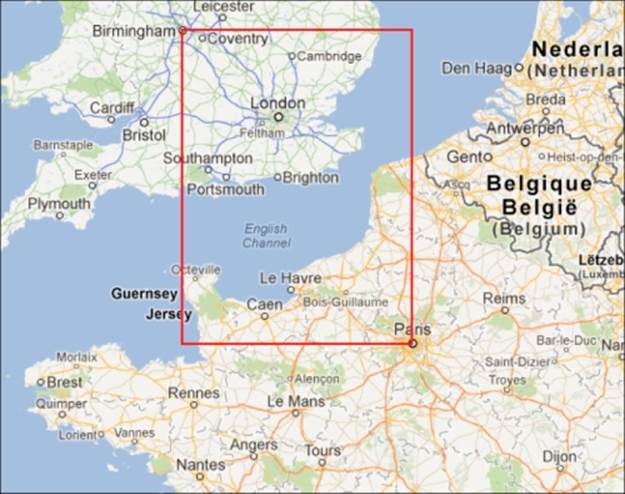
As we can see, the only city from our data that meets the criteria is London. So, let's check whether Elasticsearch knows this by running the preceding query. Let's look at the returned results, as follows:
{
"took" : 9,
"timed_out" : false,
"_shards" : {
"total" : 5,
"successful" : 5,
"failed" : 0
},
"hits" : {
"total" : 1,
"max_score" : 1.0,
"hits" : [ {
"_index" : "map",
"_type" : "poi",
"_id" : "2",
"_score" : 1.0, "_source" : { "name" : "London", "location" : [-0.1275, 51.507222] }
} ]
}
}
As you can see, again Elasticsearch agrees with the map.
Limiting the distance
The last example shows the next common requirement: limiting the results to the places that are located in the selected distance from the base point. For example, if we want to limit our results to all the cities within the 500km radius from Paris, we can use the following filter:
{
"filter" : {
"geo_distance" : {
"location" : "48.8567, 2.3508",
"distance" : "500km"
}
}
}
If everything goes well, Elasticsearch should only return a single record for the preceding query, and the record should be London; however, we will leave it for you as a reader to check.
Arbitrary geo shapes
Sometimes, using a single geographical point or a single rectangle is just not enough. In such cases, something more sophisticated is needed, and Elasticsearch addresses this by giving you the possibility to define shapes. In order to show you how we can leverage custom shape limiting in Elasticsearch, we need to modify our index and introduce the geo_shape type. Our new mapping looks as follows (we will use this to create an index called map2):
{
"poi" : {
"properties" : {
"name" : { "type" : "string", "index": "not_analyzed" },
"location" : { "type" : "geo_shape" }
}
}
}
Next, let's change our example data to match our new index structure, as follows:
{ "index" : { "_index" : "map2", "_type" : "poi", "_id" : 1 }}
{ "name" : "New York", "location" : { "type": "point", "coordinates": [-73.938611, 40.664167] }}
{ "index" : { "_index" : "map2", "_type" : "poi", "_id" : 2 }}
{ "name" : "London", "location" : { "type": "point", "coordinates": [-0.1275, 51.507222] }}
{ "index" : { "_index" : "map2", "_type" : "poi", "_id" : 3 }}
{ "name" : "Moscow", "location" : { "type": "point", "coordinates": [ 37.616667, 55.75]}}
{ "index" : { "_index" : "map2", "_type" : "poi", "_id" : 4 }}
{ "name" : "Sydney", "location" : { "type": "point", "coordinates": [151.211111, -33.865143]}}
{ "index" : { "_index" : "map2", "_type" : "poi", "_id" : 5 }}
{ "name" : "Lisbon", "location" : { "type": "point", "coordinates": [-9.142685, 38.736946] }}
The structure of the field of the geo_shape type is different from geo_point. It is syntactically called GeoJSON (http://en.wikipedia.org/wiki/GeoJSON). It allows us to define various geographical types. Let's sum up the types that we can use during querying, at least the ones that we think are the most useful ones.
Point
A point is defined by the table when the first element is the longitude and the second is the latitude. An example of such a shape can be as follows:
{
"location" : {
"type": "point",
"coordinates": [-0.1275, 51.507222]
}
}
Envelope
An envelope defines a box given by the coordinates of the upper-left and bottom-right corners of the box. An example of such a shape is as follows:
{
"type": "envelope",
"coordinates": [[ -0.087890625, 51.50874245880332 ], [ 2.4169921875, 48.80686346108517 ]]
}
Polygon
A polygon defines a list of points that are connected to create our polygon. The first and the last point in the array must be the same so that the shape is closed. An example of such a shape is as follows:
{
"type": "polygon",
"coordinates": [[
[-5.756836, 49.991408],
[-7.250977, 55.124723],
[1.845703, 51.500194],
[-5.756836, 49.991408]
]]
}
If you look closer at the shape definition, you will find a supplementary level of tables. Thanks to this, you can define more than a single polygon. In such a case, the first polygon defines the base shape and the rest of the polygons are the shapes that will be excluded from the base shape.
Multipolygon
The multipolygon shape allows us to create a shape that consists of multiple polygons. An example of such a shape is as follows:
{
"type": "multipolygon",
"coordinates": [
[[
[-5.756836, 49.991408],
[-7.250977, 55.124723],
[1.845703, 51.500194],
[-5.756836, 49.991408]
]],
[[
[-0.087890625, 51.50874245880332],
[2.4169921875, 48.80686346108517],
[3.88916015625, 51.01375465718826],
[-0.087890625, 51.50874245880332]
]]
]
}
The multipolygon shape contains multiple polygons and falls into the same rules as the polygon type. So, we can have multiple polygons and in addition to this, we can include multiple exclusion shapes.
An example usage
Now that we have our index with the geo_shape fields, we can check which cities are located in the UK. The query that will allow us to do this will look as follows:
{
"filter": {
"geo_shape": {
"location": {
"shape": {
"type": "polygon",
"coordinates": [[
[-5.756836, 49.991408], [-7.250977, 55.124723], [-3.955078, 59.352096], [1.845703, 51.500194], [-5.756836, 49.991408]
]]
}
}
}
}
}
The polygon type defines the boundaries of the UK (in a very, very imprecise way), and Elasticsearch gives the response as follows:
"hits": [
{
"_index": "map2",
"_type": "poi",
"_id": "2",
"_score": 1,
"_source": {
"name": "London",
"location": {
"type": "point",
"coordinates": [
-0.1275,
51.507222
]
}
}
}
]
As far as we know, the response is correct.
Storing shapes in the index
Usually, the shape definitions are complex, and the defined areas don't change too often (for example, the UK boundaries). In such cases, it is convenient to define the shapes in the index and use them in queries. This is possible, and we will now discuss how to do it. As usual, we will start with the appropriate mapping, which is as follows:
{
"country": {
"properties": {
"name": { "type": "string", "index": "not_analyzed" },
"area": { "type": "geo_shape" }
}
}
}
This mapping is similar to the mapping used previously. We have only changed the field name. The example data that we will use looks as follows:
{"index": { "_index": "countries", "_type": "country", "_id": 1 }}
{"name": "UK", "area": {"type": "polygon", "coordinates": [[ [-5.756836, 49.991408], [-7.250977, 55.124723], [-3.955078, 59.352096], [1.845703, 51.500194], [-5.756836, 49.991408] ]]}}
{"index": { "_index": "countries", "_type": "country", "_id": 2 }}
{"name": "France", "area": { "type":"polygon", "coordinates": [ [ [ 3.1640625, 42.09822241118974 ], [ -1.7578125, 43.32517767999296 ], [ -4.21875, 48.22467264956519 ], [ 2.4609375, 50.90303283111257 ], [ 7.998046875, 48.980216985374994 ], [ 7.470703125, 44.08758502824516 ], [ 3.1640625, 42.09822241118974 ] ] ] }}
{"index": { "_index": "countries", "_type": "country", "_id": 3 }}
{"name": "Spain", "area": { "type": "polygon", "coordinates": [ [ [ 3.33984375, 42.22851735620852 ], [ -1.845703125, 43.32517767999296 ], [ -9.404296875, 43.19716728250127 ], [ -6.6796875, 41.57436130598913 ], [ -7.3828125, 36.87962060502676 ], [ -2.109375, 36.52729481454624 ], [ 3.33984375, 42.22851735620852 ] ] ] }}
As you can see in the data, each document contains a polygon type. The polygons define the area of the given countries (again, it is far from being accurate). If you remember, the first point of a shape needs to be the same as the last one so that the shape is closed. Now, let's change our query to include the shapes from the index. Our new query will look as follows:
{
"filter": {
"geo_shape": {
"location": {
"indexed_shape": {
"index": "countries",
"type": "country",
"path": "area",
"id": "1"
}
}
}
}
}
When comparing these two queries, we can note that the shape object changed to indexed_shape. We need to tell Elasticsearch where to look for this shape. We can do this by defining the index (the index property, which defaults to shape), type (the type property), and path (the path property, which defaults to shape). The one item lacking is an id property of the shape. In our case, this is 1. However, if you want to index more shapes, we will advise you to index shapes with their name as their identifier.
The scroll API
Let's imagine that we have an index with several million documents. We already know how to build our query, when to use filters, and so on. But looking at the query logs, we see that a particular kind of query is significantly slower than the others. These queries may be using pagination. The from parameter indicates that the offsets have large values. From the application side, this can mean that users go through an enormous number of results. Often, this doesn't make sense—if a user doesn't find the desirable results on the first few pages, he/she gives up. Because this particular activity can mean something bad (possible data stealing), many applications limit the paging to dozens of pages. In our case, we assume that this is a different scenario, and we have to provide this functionality.
Problem definition
When Elasticsearch generates a response, it must determine the order of the documents that form the result. If we are on the first page, this is not a big problem. Elasticsearch just finds the set of documents and collects the first ones; let's say, 20 documents. But if we are on the tenth page, Elasticsearch has to take all the documents from pages one to ten and then discard the ones that are on pages one to nine. The problem is not Elasticsearch specific; a similar situation can be found in the database systems, for example—generally, in every system that uses the so-called priority queue.
Scrolling to the rescue
The solution is simple. Since Elasticsearch has to do some operations (determine the documents for previous pages) for each request, we can ask Elasticsearch to store this information for the subsequent queries. The drawback is that we cannot store this information forever due to limited resources. Elasticsearch assumes that we can declare how long we need this information to be available. Let's see how it works in practice.
First of all, we query Elasticsearch as we usually do. However, in addition to all the known parameters, we add one more: the parameter with the information that we want to use scrolling with and how long we suggest that Elasticsearch should keep the information about the results. We can do this by sending a query as follows:
curl 'localhost:9200/library/_search?pretty&scroll=5m' –d '{
"query" : {
"match_all" : { }
}
}'
The content of this query is irrelevant. The important thing is how Elasticsearch modifies the response. Look at the following first few lines of the response returned by Elasticsearch:
{
"_scroll_id" :
"cXVlcnlUaGVuRmV0Y2g7NTsxMDI6dklNMlkzTG1RTDJ2b25oTDNENmJzZzsxMD
U6dklNMlkzTG1RTDJ2b25oTDNENmJzZzsxMDQ6dklNMlkzTG1RTDJ2b25oTDNEN
mJzZzsxMDE6dklNMlkzTG1RTDJ2b25oTDNENmJzZzsxMDM6dklNMlkzTG1RTDJ
2b25oTDNENmJzZzswOw==",
"took" : 9,
"timed_out" : false,
"_shards" : {
"total" : 5,
"successful" : 5,
"failed" : 0
},
"hits" : {
"total" : 1341211,
…
The new part is the _scroll_id section. This is a handle that we will use in the queries that follow. Elasticsearch has a special endpoint for this: the _search/scroll endpoint. Let's look at the following example:
curl -XGET 'localhost:9200/_search/scroll?scroll=5m&pretty&scroll_id=cXVlcnlUaGVuRmV0Y2g7NTsxMjg6dklNlkzTG1RTDJ2b25oTDNENmJzZzsxMjk6dklNMlkzTG1RTDJ2b25oTDNENmJzZzsxMzA6dklNMlkzTG1RTDJ2b25oTDNENmJzZzsxMjc6dklNMlkzTG1RTDJ2b25oTDNENmJzZzsxMjY6dklNMlkzTG1RTDJ2b25oTDNENmJzZzswOw=='
Now, every call to this endpoint with scroll_id returns the next page of results. Remember that this handle is only valid for the defined time of inactivity. After the time has passed, a query with the invalidated scroll_id returns an error response, which will be similar to the following one:
{
"_scroll_id" :
"cXVlcnlUaGVuRmV0Y2g7NTsxMjg6dklNMlkzTG1RTDJ2b25oTDNENmJzZzsxMj
k6dklNMlkzTG1RTDJ2b25oTDNENmJzZzsxMzA6dklNMlkzTG1RTDJ2b25oTDNEN
mJzZzsxMjc6dklNMlkzTG1RTDJ2b25oTDNENmJzZzsxMjY6dklNMlkzTG1RTDJ2
b25oTDNENmJzZzswOw==",
"took" : 3,
"timed_out" : false,
"_shards" : {
"total" : 5,
"successful" : 0,
"failed" : 5,
"failures" : [ {
"status" : 500,
"reason" : "SearchContextMissingException[No search context
found for id [128]]"
}, {
"status" : 500,
"reason" : "SearchContextMissingException[No search context
found for id [126]]"
}, {
"status" : 500,
"reason" : "SearchContextMissingException[No search context
found for id [127]]"
}, {
"status" : 500,
"reason" : "SearchContextMissingException[No search context
found for id [130]]"
}, {
"status" : 500,
"reason" : "SearchContextMissingException[No search context
found for id [129]]"
} ]
},
"hits" : {
"total" : 0,
"max_score" : 0.0,
"hits" : [ ]
}
}
Of course, this solution is not ideal, and it is not well suited when there are many requests to random pages of various results or when the time between the requests is difficult to determine. However, you can use this successfully for use cases where you want to get larger result sets, such as transferring data between several systems.
The terms filter
One of the filters available in Elasticsearch that is very simple at first glance is the terms filter. In its simplest form, it allows you to filter documents to only those that match one of the given terms and is not analyzed. An example use of the terms filter is as follows:
{
"query" : {
"constant_score" : {
"filter" : {
"terms" : {
"title" : [ "crime", "punishment" ]
}
}
}
}
}
The preceding query would result in documents that match the crime or punishment terms in the title field. The way the terms filter works is that it iterates over the provided terms and finds the documents that match these terms. Of course, the matched document identifiers are loaded into a structure called bitset and are cached. Sometimes, we may want to alter the default behavior. We can do this by providing the execution parameter with one of the following values:
· plain: This is the default method that iterates over all the terms provided, storing the results in a bitset and caching them.
· fielddata: This value generates term filters that use the fielddata cache to compare terms. This mode is very efficient when filtering on the fields that are already loaded into the fielddata cache—for example, the ones used for sorting, faceting, or warming using index warmers. This execution mode can be very effective when filtering on a large number of terms.
· bool: This value generates a term filter for each term and constructs a bool filter from the generated ones. The constructed bool filter is not cached because it can execute the term filters that were constructed and were already cached.
· and: This value is similar to the bool value, but Elasticsearch constructs the and filter instead of the bool filter.
· or: This value is similar to the bool value, but Elasticsearch constructs the or filter instead of the bool filter.
An example query with the execution parameter can look like the following:
{
"query" : {
"constant_score" : {
"filter" : {
"terms" : {
"title" : [ "crime", "punishment" ],
"execution" : "and"
}
}
}
}
}
Terms lookup
We are talking about the terms filter not because of its ability to filter documents but because of the terms lookup functionality added in Elasticsearch 0.90.6. Instead of passing the list of terms explicitly, the terms lookup mechanism can be used to load the terms from a provided source. To illustrate how it works, let's create a new index and index three documents by using the following commands:
curl -XPOST 'localhost:9200/books/book/1' -d '{
"id" : 1,
"name" : "Test book 1",
"similar" : [ 2, 3 ]
}'
curl -XPOST 'localhost:9200/books/book/2' -d '{
"id" : 2,
"name" : "Test book 2",
"similar" : [ 1 ]
}'
curl -XPOST 'localhost:9200/books/book/3' -d '{
"id" : 3,
"name" : "Test book 3",
"similar" : [ 1, 3 ]
}'
Now, let's assume that we want to get all the books that are similar to the book with the identifier equal to 3. Of course, we can first get the third book, get the value for the similar field, and run another query. But let's do it using the terms lookup functionality; basically, we will let Elasticsearch retrieve the document and load the value of the similar field for us. To do this, we can run the following command:
curl -XGET 'localhost:9200/books/_search?pretty' -d '{
"query" : {
"filtered" : {
"query" : {
"match_all" : {}
},
"filter" : {
"terms" : {
"id" : {
"index" : "books",
"type" : "book",
"id" : "3",
"path" : "similar"
},
"_cache_key" : "books_3_similar"
}
}
}
},
"fields" : [ "id", "name" ]
}'
The response to the preceding command will be as follows:
{
"took" : 2,
"timed_out" : false,
"_shards" : {
"total" : 5,
"successful" : 5,
"failed" : 0
},
"hits" : {
"total" : 2,
"max_score" : 1.0,
"hits" : [ {
"_index" : "books",
"_type" : "book",
"_id" : "1",
"_score" : 1.0,
"fields" : {
"id" : 1,
"name" : "Test book 1"
}
}, {
"_index" : "books",
"_type" : "book",
"_id" : "3",
"_score" : 1.0,
"fields" : {
"id" : 3,
"name" : "Test book 3"
}
} ]
}
}
As you can see in the preceding response, we got exactly what we wanted: the books with the identifiers 1 and 3. Of course, the terms lookup mechanism is highly optimized—the cache information will be used if the information is present and so on. Also, the_cache_key property is used to specify the key under which the cached results for the terms lookup will be stored. It is advisable to set it in order to be able to easily clear the cache if needed. Of course the _cache_key property value should be different for different queries.
Note
Note that the _source field needs to be stored for the terms lookup functionality to work.
The terms lookup query structure
Let's recall our terms lookup filter that we used in order to discuss the query to fully understand it:
"filter" : {
"terms" : {
"id" : {
"index" : "books",
"type" : "book",
"id" : "3",
"path" : "similar"
},
"_cache_key" : "books_3_similar"
}
}
We used a simple filtered query, with the query matching all the documents and the terms filter. We are filtering the documents using the id field because of the name of the object that groups all the other properties in the filter. In addition to this, we've used the following properties:
· index: This specifies from which index we want the terms to be loaded. In our case, it's the books index.
· type: This specifies the type that we are interested in, which in our case, is the book type.
· id: This specifies the identifier of the documents we want the terms list to be fetched from. In our case, it is the document with the identifier 3.
· path: This specifies the field name from which the terms should be loaded, which is the similar field in our query.
What's more is that we are allowed to use two more properties, which are as follows:
· routing: This specifies the routing value that should be used by Elasticsearch when loading the terms to the filter.
· cache: This specifies whether Elasticsearch should cache the filter built from the loaded documents. By default, it is set to true, which means that Elasticsearch will cache the filter.
Note
Note that the execution property is not taken into account when using the terms lookup mechanism.
Terms lookup cache settings
Elasticsearch allows us to configure the cache used by the terms lookup mechanism. To control the mentioned cache, one can set the following properties in the elasticsearch.yml file:
· indices.cache.filter.terms.size: This defaults to 10mb and specifies the maximum amount of memory that Elasticsearch can use for the terms lookup cache. The default value should be enough for most cases; however, if you know that you'll load vast amount of data into it, you can increase it.
· indices.cache.filter.terms.expire_after_access: This specifies the maximum time after which an entry should expire after it is last accessed. By default, it is disabled.
· indices.cache.filter.terms.expire_after_write: This specifies the maximum time after which an entry should be expired after it is put into the cache. By default, it is disabled.
Summary
In this chapter, we learned more things about Elasticsearch data analysis capabilities. We used aggregations and faceting to bring meaning to the data we indexed. We also introduced the spellchecking and autocomplete functionalities to our application by using the Elasticsearch suggesters. We created the alerting functionality by using a percolator, and we indexed binary files by using the attachment functionality. We indexed and searched geospatial data and used the scroll API to efficiently fetch a large number of results. Finally, we used the terms lookup mechanism to speed up the querying process that fetches a list of terms.
In the next chapter, we'll focus on Elasticsearch clusters and how to handle them. We'll see what node discovery is, how it is used, and how to alter its configuration. We'll learn about the gateway and recovery modules, and we will alter their configuration. We will also see what the buffers in Elasticsearch are, where they are used, and how to configure them. We will prepare our cluster for a high indexing and querying throughput, and we will use index templates and dynamic mappings.
All materials on the site are licensed Creative Commons Attribution-Sharealike 3.0 Unported CC BY-SA 3.0 & GNU Free Documentation License (GFDL)
If you are the copyright holder of any material contained on our site and intend to remove it, please contact our site administrator for approval.
© 2016-2026 All site design rights belong to S.Y.A.