Anonymizing Health Data: Case Studies and Methods to Get You Started (2013)

Chapter 6. Longitudinal Events Data: A Disaster Registry

Complex health data sets contain information about patients over periods of time. A person’s medical history can be taken as a series of events: when they were first diagnosed with a disease, when they received treatment, when they were admitted to an emergency department. Our case study for this chapter is the World Trade Center (WTC) disaster registry. The collapse of the Twin Towers at the World Trade Center is one of those unforgettable disasters that has deeply affected many people, both locally and abroad. The Clinical Center of Excellence at Mount Sinai has been following WTC workers and volunteers for years in an effort to provide them with the best treatment for the physical and mental health conditions related to their WTC service.^[51^] As the saying goes, you can’t manage what you don’t measure.

NOTE

We’ll be using the term “events” to refer to a patient’s medical information in this discussion because of the structure of the WTC data. But the methods we explore here apply equally well to other data sets, such as discharge data or claims data. When we get to the methods themselves, we’ll point out how they apply to these other scenarios, if the differences need to be highlighted.

In looking at this longitudinal disaster registry, we need to revisit the assumptions we make about what an adversary can know to re-identify patients in a data set. We started with an adversary that knows all, then relaxed some of our assumptions in Chapter 4 (an adversary can’t know everything, or we might as well pack it in). What we need is a way to measure average risk when the adversary doesn’t know all. What we need is the concept of adversary power.

Adversary Power

A patient can have multiple events related to a medical case, such as the multiple procedures the patient has undergone or diseases he has been diagnosed with. But it would be overly paranoid to assume that an adversary knows all of these things. The adversary may know that someone fainted and was admitted on a certain day, but know neither the diagnosis codes for everything the doctors wrote down about the patient, nor all the procedures performed.

So it’s reasonable to assume that an adversary will have information on only a subset of these events. The amount of information the adversary has is known as the power of the adversary, and we use this idea to estimate the risk of re-identification. We don’t know what type of adversary we might be dealing with, so we have to assume all of the plausible attacks described in Measuring Risk Under Plausible Attacks (except for the public data release, which would require using maximum risk).

The power of the adversary reflects the number of events about which the adversary has some background information. It applies only to the longitudinal events (level 2) and not to the basic information about patients, like their demographics (level 1). This basic level 1 information about patients is assumed to be known, the same as it would be if we were working with a cross-sectional data set on its own (like we did in Chapter 3).

Now, if there’s only one quasi-identifier in the level 2 events, the adversary power is the number of values that the adversary is assumed to know in that quasi-identifier. For example, if the quasi-identifier is the diagnosis code, the power is the number of diagnosis codes that the adversary knows.

A power of p therefore translates into p quasi-identifier values that can be used for re-identifying patients. If there’s more than one quasi-identifier, the adversary power is the number of values that the adversary is assumed to know in each quasi-identifier. A power of p this time translates intop quasi-identifier values times the number of quasi-identifiers. So two quasi-identifiers means 2 × p pieces of information that can be used by the adversary for re-identifying a patient.

So, if the date of diagnosis is one quasi-identifier and the diagnosis itself is another, the adversary would know the dates for p events and the diagnoses for another p events. The events might overlap, or they might not—it depends on how we decide to sample for adversary power (which we’ll get to in A Sample of Power). But all in all, the adversary has 2 × p pieces of background information for a patient.

Keeping Power in Check

Previous efforts that considered adversary power always assumed that the power was fixed for all patients.^[52^] But intuitively, it makes sense that the adversary would have different amounts of background knowledge for different patients. Everything else being equal, it’s easier to have background information about a patient with a large number of events than about a patient with few events. Therefore, we expect power to increase with the number of events that a patient has undergone.

Also, it’s likely that certain pieces of background information are more easily knowable than others by an adversary, making it necessary to treat the quasi-identifiers separately when it comes to computing adversary power. For example, it would be easier to know diagnosis values for patients with chronic conditions whose diagnoses keep repeating across visits than to know diagnosis values for patients who have a variety of different ailments.

Further, if the adversary knows the information in one visit, she can more easily predict the information in other visits, increasing the amount of background knowledge that she has. So, the diversity of values on a quasi-identifier across a patient’s visits becomes an important consideration. And we therefore expect the power of an adversary to decrease with the diversity of values on the quasi-identifiers.

To capture these differences, we break patients into four groups, shown in Table 6-1. For patients with few medical events and high variability between those events, little background information will be available to an adversary, who consequently will have a lower level of adversary power. For patients with many medical events and low variability between those events, more background information will be available to an adversary, giving him a higher level of adversary power. The other combinations fall in between.

Table 6-1. I’ve got the power, oh Snap! Of course, the power values are just to illustrate relative size—this changes based on max power.

Power in Practice

We let p_max be the maximum power assumed of an adversary, n be the number of events for the patient, and v be the variability of the quasi-identifier for the patient. Then, for each patient, we calculate the adversary power for each quasi-identifier:

Adversary power for quasi-identifier (applied to a single patient)

p = ⌈1 + (p_max – 1) × (n / v) / max_patients(n / v)⌉

The max function is over all patients, because we want to scale adversary power based on the highest ratio of n over v. The variability v ranges from 0 for no variability (i.e., the quasi-identifier never changes value) to 1 for maximum variability (i.e., the quasi-identifier is always changing), and is a probability derived from the Simpson index.^[53^]

Just to explain the equation and the logic behind it a bit more, we start with a value of 1 in computing adversary power because we have to start somewhere. We don’t want to assume that the adversary knows absolutely nothing about a patient! The rest of the equation involves scaling the range of power values, so that the adversary power goes from 1 to a max that we define, our so-called p_max (whereas everything else in the equation is determined from the data). We also round up (e.g., 1.1 becomes 2) so that we assume the adversary has more power rather than less.

Which brings us to an important question: what is the maximum possible power? For longitudinal data sets with multiple quasi-identifiers, we typically use a max power of 5 per quasi-identifier.^[54^] It’s not uncommon for us to have anywhere between 5 and 10 quasi-identifiers to work with, which means a maximum power of anywhere from 5 × 5 = 25 to 5 × 10 = 50 pieces of background information about a single patient.

Oh great lobster in the sky, 50 pieces of background info about a single patient? That’s a lot of medical information to know about someone! To think that this is less than knowing all of a patient’s medical history really puts things into perspective—there can be a lot of information in longitudinal health data. That’s why we’re trying to scale back our assumptions to a more reasonable level of what an adversary could know.

A Sample of Power

We sample patients’ quasi-identifier values so that we can use their background information to simulate an attack on the data. Typically we randomly sample from 1,000 to 5,000 patients in a data set, collect our sample of their background information, then see how many patients we can match to in the full data set. The proportion of unique matches out of our sample of patients is a form of average risk. We consider three ways to sample a patient’s background information, and each has its pros and cons:

Random sample per quasi-identifier

This is a no-brainer. Random sampling is always the first approach when sampling. The problem with it in this case is that health data is always strongly correlated across records. A record can have multiple fields related to an event, and a patient can have many records in a longitudinal data set. If we have diseases in one column and procedures in another, a random sample of one may in fact imply the other. But since they are sampled independently of one another, we end up with twice the amount of information about each (unless there’s significant overlap between the two samples).

Let’s say we have a hernia (ouch!) in the disease sample. This implies a hernia repair, but we may not have sampled that in the procedures for this patient. Then we have 12 stitches on the left arm in the procedures sample, implying a lacerated arm—but we may not have sampled that in the diseases for this patient. As shown in Table 6-2, a sample of only one value in each of two fields resulted in four pieces of background information, instead of two.

Table 6-2. A power of 1 means one disease, one procedure (bold = sampled)

Record sample

OK, so a random sample of each quasi-identifier might result in us assuming that the adversary has more background information than was intended, due to the strong correlation of health data across records. The obvious solution is therefore to sample by record! That way a hernia and its repair are in the same basket of information about the patient (Table 6-3). But isn’t that cheating, because we now have less background information since one implies the other? Well, that’s true only for strongly correlated information.

Sampling by record captures the connections between quasi-identifiers without us having to do it ourselves. Also, it’s not likely for one piece of information in a quasi-identifier to imply all the others in the record. The lacerated arm could have been stitched up in an ambulance, an emergency room, or even a walk-in clinic. And odd pairings of disease and procedure will still stand out.

Table 6-3. Ah, this time we sample the record to get one disease, one procedure.

Sample by visit

Another option is to sample by visit, so that we get a random sample of each quasi-identifier limited to a visit. This gives us a random sample, and the correlation of health information is in the sample so that it doesn’t unintentionally inflate power. But in this case it’s the correlation within a visit rather than a record. This approach is a bit more complicated, though, because we need to consider the diversity of the visits themselves, how many visits to sample, and how much information to sample per visit.

When sampling by visit, we also need a way to identify visits. Some data sets will have a visit identifier, so that we can track a visit over several days, but some data sets won’t have this info. This isn’t our preferred approach to sampling quasi-identifiers because it raises more questions than answers, especially when dealing with a wide range of data sets from different sources.

We prefer to sample by record. And once we have our sample of a patient’s quasi-identifier values, we treat it as a basket of information for matching against all patients in a data set. The way the information was gathered is lost. We don’t care about order, or visits, or claims. We just care about the information in the basket. In other words, we’re assuming the adversary doesn’t know how all the information is joined together.

Now, if we want two pieces of information from different quasi-identifiers to be connected, so that what happens to one also applies to the other, we define them as connected quasi-identifiers so that they aren’t treated as two independent sources of information. We saw this concept inConnected Variables, and we’ll see an example of it in the WTC disaster registry (it’s easier to explain using an example).

The WTC Disaster Registry

Over 50,000 people are estimated to have helped with the rescue and recovery efforts after 9/11, and the medical records of over 27,000 of those are captured in the WTC disaster registry created by the Clinical Center of Excellence at Mount Sinai. Working with a variety of organizations, they reached out to recruit 9/11 workers and volunteers. Everyone who has participated in the registry has gone through a comprehensive series of examinations.^[55^] These include:

§ Medical questionnaires

§ Mental-health questionnaires

§ Exposure assessment questionnaires

§ Standardized physical examinations

§ Optional follow-up assessments every 12 to 18 months

Capturing Events

We needed to convert the questionnaires and exams into a longitudinal data set we could work with—our methods don’t apply directly to questionnaire data. So we needed to convert questions and exams into data we could process, then map the generalizations and suppression back to the questionnaires and exams. The registry is comprehensive and includes a lot of historical information gathered from patients. Unlike claims data, the WTC data contains no disease or procedure codes, no places of service (besides Mount Sinai), and no rows of information that organize the data set.

Instead, the registry presents a collection of health events, including information about when a specific health-related item is not a problem. That’s something you don’t see in claims data, unless there’s a charge for that health-related item. Imagine an insurer charging you for not having a disease, or charging you for still having a disease even though you’re not getting treatment for it! But since this kind of data is in the registry, and could be known to an adversary, we counted these as events.

After 9/11, the workers and volunteers became well known in their communities for their heroic efforts. This makes the information about them more prevalent, so we decided to connect the events to their respective dates. The visit date was used for questions that were specific to the date at which the visit occurred.

Thus, “Do you currently smoke?” would create an event for smoking at the time of visit, and “Have you been diagnosed with this disease?” would create an event for “no diagnosis” at the time of visit if the patient answered “no” to the question. Some questions included dates that could be used directly with the quasi-identifier and were more informative than the visit date. For example, the answer to “When were you diagnosed with this disease?” was used to provide a date for the disease event.

Ten years after the fact, however, it seems unlikely that an adversary will know the dates of a patient’s events before 9/11. Often patients gave different years of diagnosis on follow-up visits because they themselves didn’t remember what medical conditions they had! So instead of the date of event, we used “pre-9/11” as a value. But we made a distinction between childhood (under 18) and adulthood (18 and over) diagnoses, because this seemed like something an adversary could reasonably know.

These generalizations were done only for measuring risk, and weren’t applied to the de-identified registry data. If the date can’t be known to the adversary, there’s no point in removing it from the original data. But before we get lambasted for this assumption, don’t think that we left all those dates in their exact form in the data! We masked all dates to the same level of generalization that we used for the other events in the data, which we’ll get to in the risk assessment.

The WTC Data Set

We’ll start with the level 1 demographic data, because this is the data we assume to be known to an adversary (i.e., we don’t use adversary power on level 1 data). The level 1 data in the registry already included generalizations used in the analyses conducted by Mount Sinai researchers. For example, date of birth was recorded for each patient, but the data set we received also included 5- and 10-year age groups. These generalizations were included because it’s what researchers at Mount Sinai were using in their work.

We took the most general levels of the level 1 data available right off the bat. We did this because we knew, given all the background information about patients, that the risk of re-identification would be high. The only generalization we added was to divide height into four possible groups (<10th percentile, 10th to <50th percentile, 50th to <90th percentile, 90th percentile and higher).

Of course, if the risk had been well below our threshold, with minimal amounts of suppression, we would have gone back to try less general pieces of information (this didn’t happen). But this seemed like a good starting point, since the level 1 data was already generalized to levels that were acceptable in the research being done at Mount Sinai.

The specific generalizations that were in the data aren’t important, but the final level 1 data in Table 6-4 certainly is. This is because we include all level 1 data as part of what we assume an adversary knows, and because the more specific the demographic information is, the more identifiable a patient becomes.

Table 6-4. Level 1 quasi-identifiers

The registry included a lot of information about patients, so we can give you only a taste of the level 2 event data in Table 6-5. We divided the events into three categories (based on the structure of the questionnaires and data): variable demographics, diseases (including mental health), and WTC exposures and activities.

Table 6-5. A sample of the possible events

The Power of Events

We specified a power level for each series of events. We chose a total power of 15 for longitudinal event data: a power of 5 for variable demographics, a power of 5 for disease events, and a power of 5 for mental health events. This means we assumed that an adversary would know up to 15 events about each individual in the registry.

The variability of patient events is at its maximum under this setup (i.e., v = 1), because we didn’t include periods during which there was no change in a patient’s quasi-identifiers, and we did include the year of the event in our analysis. If a patient was married in 2002 and divorced in 2006, we included this information as two events: 2002 married, and 2006 divorced. The patient’s marital status could either be inferred or is missing for all other years, and therefore provides no further information. But there’s no set of events (married, married, married), so variability is never “low.”

Because we now have three main areas of patient information—variable demographics, diseases (including mental health), and 9/11 exposures—we assume a max adversary power of 15. Don’t forget that we always include a patient’s level 1 fixed demographics.

Adversary power applies to the longitudinal data only. This isn’t a book of equations, but it’s interesting (we think!) to see how our equation for adversary power works in this application. We have determined that p_max is 15, so we plug in (p_max – 1) = 14, and take out v because a divisor of 1 has no effect on the equation:

Adversary power (applied to WTC patient events)

p = ⌈1 + 14 × n / max_patients(n)⌉

Actually, there’s a detail we skipped over. It’s possible that patients with an abnormally high number of events could skew the equation. So, to get rid of outliers, we take the max to be the mean number of events per patient plus two standard deviations. For the WTC registry the mean number of events per patient was 103.8 (the median was 98), with a standard deviation of 52.7. This gives us a “max” of 209.2 events (the real max was 260, which just goes to show how much it can be skewed by an outlier):

Adversary power (applied to WTC patient events, no outliers)

p = ⌈1 + 14 × n / 209.2⌉

Given that the median number of events per patient was 98, half the patients had an adversary power of 1 to 8, and half had an adversary power of 9 to 15. That works out quite well. So, the more visits they attended, the higher the adversary power. This is exactly the way we want adversary power to work. The distribution of events in Figure 6-1 clearly shows the five visits in the data we looked at, and adversary power works out to be:

§ 3–4 for one visit

§ 7–8 for two visits

§ 11–12 for three visits

§ 14–15 for four visits

§ 15 for five or more visits (power is at its maximum at this point)

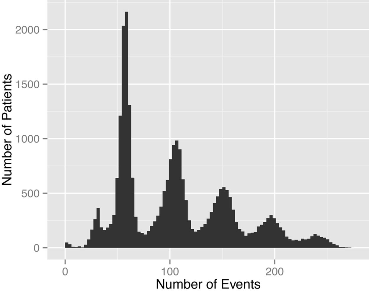
Figure 6-1. A roller coaster of events! The peaks represent the five visits, which show fewer and fewer patients attending follow-ups.

This change in power makes intuitive sense and captures the increase in background knowledge that an adversary would have as the number of patient visits rises. But the increase in adversary knowledge also affects fewer patients.

Risk Assessment

Now we’re back to applying our methodology from Chapter 2. First and foremost, agreements were in place to limit the distribution of the data to a group of analysts, and these agreements prohibited the re-identification of individuals in the registry. The agreements also stipulated that if anyone in the registry were inadvertently identified, that information could not be disclosed to anyone. Period. Full stop.

Originally, Mount Sinai wanted the data to be treated as a public data release, which would warrant an overall risk threshold of 0.1. But the data was not being made public, and there were strong agreements in place, so we decided that an average risk of 0.15 would be appropriate.

Threat Modeling

Let’s take a look at our three threats for this data set:

1. Because motives and capacity are low, but the extent of mitigating controls is also low, Pr(attempt) = 0.4. Basically, there are two ways that a re-identification attack might be launched: either through a deliberate attempt by the analyst, which is pretty unlikely given the explicit prohibition in the agreements, or through poor control over how data is handled, making it possible for someone on-site to attempt to re-identify the data. We assumed that the data users would only have to meet the HIPAA Security Rule requirements (see Implementing the HIPAA Security Rule for more details on these).

2. You would probably be aware of it if someone you knew was a WTC first responder, since they did something truly awesome, and therefore so would an adversary. And given all the publicity and outreach involved in recruiting people, it’s fair to assume that an adversary knows whether that person is also in the WTC registry. The probability of knowing a person in New York City who is in the WTC registry of 27,000 patients is Pr(acquaintance) = 0.39.

3. Pr(breach) = 0.27, based on our good old (for this book) historical data.

Results

Using adversary power, we were able to get the average risk below our threshold of 0.15 with some generalization and suppression, but nothing too crazy. We had to use the most generalized form of the level 1 data that was already provided by Mount Sinai, and we generalized dates to years (except the start dates of WTC efforts and service hours). Now, that might seem like a lot of generalization for dates, but keep in mind we’re talking about either historical diagnoses, or the five visits (baseline plus follow-up). So, it’s good enough for the analyses being considered.

There was also some suppression, but overall it worked out to be only 1% of the cells in the questionnaires. Now, because the level 1 data is always assumed to be known, it’s almost always the case that this is the data that gets the most generalization and suppression. But this is way better than what would be achieved without power. In fact, we doubt that meaningful data can be disclosed at all without considering adversary power during the de-identification.

Final Thoughts

Adversary power is a great way to scale back our assumptions on longitudinal data from the “all-knowing” to the “some-knowing” adversary. Sampling the longitudinal data and scaling it based on the number and variability of the data is an extremely useful way to measure average risk. Keep in mind, though, that we don’t apply these techniques blindly. If we know the data is out there somewhere, say publicly, and there’s a risk that a data set will be matched to other data sets, then of course we need to go back a step and assume some form of omniscient adversary.

But in many cases, where there are controls on data (which is the case for many commercial data sets), this is the way to go. It allows us to decrease the amount of generalization and suppression needed to produce data sets that are useful for analytics. So it’s a staple in our tool belt; you could say it’s our power tool (ouch, bad pun!).