High Performance MySQL (2012)
Chapter 9. Operating System and Hardware Optimization
Your MySQL server can perform only as well as its weakest link, and the operating system and the hardware on which it runs are often limiting factors. The disk size, the available memory and CPU resources, the network, and the components that link them all limit the system’s ultimate capacity. Thus, you need to choose your hardware carefully, and configure the hardware and operating system appropriately. For example, if your workload is I/O-bound, one approach is to design your application to minimize MySQL’s I/O workload. However, it’s often smarter to upgrade the I/O subsystem, install more memory, or reconfigure existing disks.
Hardware changes very rapidly, so anything we write about particular products or components in this chapter will become outdated quickly. As usual, our goal is to help improve your understanding so that you can apply your knowledge in situations we don’t cover directly. However, we will use currently available hardware to illustrate our points.
What Limits MySQL’s Performance?
Many different hardware components can affect MySQL’s performance, but the two most frequent bottlenecks we see are CPU and I/O saturation. CPU saturation happens when MySQL works with data that either fits in memory or can be read from disk as fast as needed. A lot of datasets fit completely in memory with the large amounts of RAM available these days.
I/O saturation, on the other hand, generally happens when you need to work with much more data than you can fit in memory. If your application is distributed across a network, or if you have a huge number of queries and/or low latency requirements, the bottleneck might shift to the network instead.
The techniques shown in Chapter 3 will help you find your system’s limiting factor, but look beyond the obvious when you think you’ve found a bottleneck. A weakness in one area often puts pressure on another subsystem, which then appears to be the problem. For example, if you don’t have enough memory, MySQL might have to flush caches to make room for data it needs—and then, an instant later, read back the data it just flushed (this is true for both read and write operations). The memory scarcity can thus appear to be a lack of I/O capacity. When you find a component that’s limiting the system, ask yourself, “Is the component itself the problem, or is the system placing unreasonable demands on this component?” We explored this question in our diagnostics case study in Chapter 3.
Here’s another example: a saturated memory bus can appear to be a CPU problem. In fact, when we say that an application has a “CPU bottleneck” or is “CPU-bound,” what we really mean is that there is a computational bottleneck. We delve into this issue next.
How to Select CPUs for MySQL
You should consider whether your workload is CPU-bound when upgrading current hardware or purchasing new hardware.
You can identify a CPU-bound workload by checking the CPU utilization, but instead of looking only at how heavily your CPUs are loaded overall, look at the balance of CPU usage and I/O for your most important queries, and notice whether the CPUs are loaded evenly. You can use the tools discussed later in this chapter to figure out what limits your server’s performance.
Which Is Better: Fast CPUs or Many CPUs?
When you have a CPU-bound workload, MySQL generally benefits most from faster CPUs (as opposed to more CPUs).
This isn’t always true, because it depends on the workload and the number of CPUs. Older versions of MySQL had scaling issues with multiple CPUs, and even new versions cannot run a single query in parallel across many CPUs. As a result, the CPU speed limits the response time for each individual CPU-bound query.
When we discuss CPUs, we’re a bit casual with the terminology, to help keep the text easy to read. Modern commodity servers usually have multiple sockets, each with several CPU cores (which have independent execution units), and each core might have multiple “hardware threads.” These complex architectures require a bit of patience to understand, and we won’t always draw clear distinctions among them. In general, though, when we talk about CPU speed we’re really talking about the speed of the execution unit, and when we mention the number of CPUs we’re referring to the number that the operating system sees, even though that might be a multiple of the number of independent execution units.
Modern CPUs are much improved over those available a few years ago. For example, today’s Intel CPUs are much faster than previous generations, due to advances such as directly attached memory and improved interconnects to devices such as PCIe cards. This is especially good for very fast storage devices, such as Fusion-io and Virident PCIe flash drives.
Hyperthreading also works much better now than it used to, and operating systems know how to use hyperthreading quite well these days. It used to be that operating systems weren’t aware when two virtual CPUs really resided on the same die and would schedule tasks on two virtual processors on the same physical execution unit, believing them to be independent. Of course, a single execution unit can’t really run two processes at the same time, so they’d conflict and fight over resources. Meanwhile, the operating system would leave other CPUs idle, thus wasting power. The operating system needs to be hyperthreading-aware because it has to know when the execution unit is actually idle, and switch tasks accordingly. A common cause of such problems used to be waits on the memory bus, which can take up to a hundred CPU cycles and is analogous to an I/O wait at a very small scale. That’s all much improved in newer operating systems. Hyperthreading now works fine; we used to advise people to disable it sometimes, but we don’t do that anymore.
All this is to say that you can get lots of fast CPUs now—many more than you could when we published the second edition of this book. So which is best, many or fast? Usually, you want both. Broadly speaking, you might have two goals for your server:
Low latency (fast response time)
To achieve this you need fast CPUs, because each query will use only a single CPU.
High throughput
If you can run many queries at the same time, you might benefit from multiple CPUs to service the queries. However, whether this works in practice depends on your situation. Because MySQL doesn’t scale perfectly on multiple CPUs, there is a limit to how many CPUs you can use anyway. In older versions of the server (up to late releases of MySQL 5.1, give or take) that was a serious limitation. In newer versions, you can confidently scale to 16 or 24 CPUs and perhaps beyond, depending on which version you’re using (Percona Server tends to have a slight edge here).
If you have multiple CPUs and you’re not running queries concurrently, MySQL can still use the extra CPUs for background tasks such as purging InnoDB buffers, network operations, and so on. However, these jobs are usually minor compared to executing queries.
MySQL replication (discussed in the next chapter) also works best with fast CPUs, not many CPUs. If your workload is CPU-bound, a parallel workload on the master can easily serialize into a workload the replica can’t keep up with, even if the replica is more powerful than the master. That said, the I/O subsystem, not the CPU, is usually the bottleneck on a replica.
If you have a CPU-bound workload, another way to approach the question of whether you need fast CPUs or many CPUs is to consider what your queries are really doing. At the hardware level, a query can either be executing or waiting. The most common causes of waiting are waiting in the run queue (when the process is runnable, but all the CPUs are busy), waiting for latches or locks, and waiting for the disk or network. What do you expect your queries to be waiting for? If they’ll be waiting for latches or locks, you generally need faster CPUs; if they’re waiting in the run queue, then either more or faster CPUs will help. (There might be exceptions, such as a query waiting for the InnoDB log buffer mutex, which doesn’t become free until the I/O completes—this might indicate that you actually need more I/O capacity.)
That said, MySQL can use many CPUs effectively on some workloads. For example, suppose you have many connections querying distinct tables (and thus not contending for table locks, which can be a problem with MyISAM and Memory tables), and the server’s total throughput is more important than any individual query’s response time. Throughput can be very high in this scenario because the threads can all run concurrently without contending with each other.
Again, this might work better in theory than in practice: InnoDB has global shared data structures regardless of whether queries are reading from distinct tables or not, and MyISAM has global locks on each key buffer. It’s not just the storage engines, either; InnoDB used to get all the blame, but some of the improvements it’s received lately have exposed other bottlenecks at higher levels in the server. The infamous LOCK_open mutex can be a real problem on MySQL 5.1 and older versions; ditto for some of the other server-level mutexes (the query cache, for example).
You can usually diagnose these types of contention with stack traces. See the pt-pmp tool in Percona Toolkit, for example. If you encounter such problems, you might have to change the server’s configuration to disable or alter the offending component, partition (shard) your data, or change how you’re doing things in some way. There are too many possible problems and corresponding solutions for us to list them all, but fortunately, the answer is usually obvious once you have a firm diagnosis. Also fortunately, most of the problems are edge cases you’re unlikely to encounter; the most common cases are being fixed in the server itself as time passes.
CPU Architecture
Probably upwards of 99% of MySQL server instances (excluding embedded usage) run on the x86 architecture, on either Intel or AMD chips. This is what we focus on in this book, for the most part.
Sixty-four-bit architectures are now the default, and it’s hard to even buy a 32-bit CPU these days. MySQL works fine on 64-bit architectures, though some things didn’t become 64-bit capable for a while, so if you’re using an older version of the server, you might need to take care. For example, in early MySQL 5.0 releases, each MyISAM key buffer was limited to 4 GB, the size addressable by a 32-bit integer. (You can create multiple key buffers to work around this, though.)
Make sure you use a 64-bit operating system on your 64-bit hardware! It’s less common these days than it used to be, but for a while most hosting providers would install 32-bit operating systems on servers even when the servers had 64-bit CPUs. This meant that you couldn’t use a lot of memory: even though some 32-bit systems can support large amounts of memory, they can’t use it as efficiently as a 64-bit system, and no single process can address more than 4 GB of memory on a 32-bit system.
Scaling to Many CPUs and Cores
One place where multiple CPUs can be quite helpful is an online transaction processing (OLTP) system. These systems generally do many small operations, which can run on multiple CPUs because they’re coming from multiple connections. In this environment, concurrency can become a bottleneck. Most web applications fall into this category.
OLTP servers generally use InnoDB, which has some unresolved concurrency issues with many CPUs. However, it’s not just InnoDB that can become a bottleneck: any shared resource is a potential point of contention. InnoDB gets a lot of attention because it’s the most common storage engine for high-concurrency environments, but MyISAM is no better when you really stress it, even when you’re not changing any data. Many of the concurrency bottlenecks, such as InnoDB’s row-level locks and MyISAM’s table locks, can’t be optimized away internally—there’s no solution except to do the work as fast as possible, so the locks can be granted to whatever is waiting for them. It doesn’t matter how many CPUs you have if a single lock is causing them all to wait. Thus, even some high-concurrency workloads benefit from faster CPUs.
There are actually two types of concurrency problems in databases, and you need different approaches to solve them:
Logical concurrency issues
Contention for resources that are visible to the application, such as table or row locks. These problems usually require tactics such as changing your application, using a different storage engine, changing the server configuration, or using different locking hints or transaction isolation levels.
Internal concurrency issues
Contention for resources such as semaphores, access to pages in the InnoDB buffer pool, and so on. You can try to work around these problems by changing server settings, changing your operating system, or using different hardware, but you might just have to live with them. In some cases, using a different storage engine or a patch to a storage engine can help ease these problems.
The number of CPUs MySQL can use effectively and how it scales under increasing load—its “scaling pattern”—depend on both the workload and the system architecture. By “system architecture,” we mean the operating system and hardware, not the application that uses MySQL. The CPU architecture (RISC, CISC, depth of pipeline, etc.), CPU model, and operating system all affect MySQL’s scaling pattern. This is why benchmarking is so important: some systems might continue to perform very well under increasing concurrency, while others perform much worse.
Some systems can even give lower total performance with more processors. This used to be quite common; we know of many people who tried to upgrade to systems with more CPUs, only to be forced to revert to the older systems (or bind the MySQL process to only some of the cores) because of lower performance. In the MySQL 5.0 days, before the advent of the Google patches and then Percona Server, the magic number was 4 cores, but these days we’re seeing people running on servers with up to 80 “CPUs” reported to the operating system. If you’re planning a big upgrade, you’ll have to consider your hardware, server version, and workload.
Some MySQL scalability bottlenecks are in the server, whereas others are in the storage engine layer. How the storage engine is designed is crucial, and you can sometimes switch to a different storage engine and get more from multiple CPUs.
The processor speed wars we saw around the turn of the century have subsided to some extent, and CPU vendors are now focusing more on multicore CPUs and variations such as multithreading. The future of CPU design might well be hundreds of processor cores; quad-core and hex-core CPUs are common today. Internal architectures vary so widely across vendors that it’s impossible to generalize about the interaction between threads, CPUs, and cores. How the memory and bus are designed is also very important. In the final analysis, whether it’s better to have multiple cores or multiple physical CPUs is also architecture-specific.
Two other complexities of modern CPUs deserve mention. Frequency scaling is the first. This is a power management technique that changes the CPU clock speed dynamically, depending on the demand placed on the CPU. The problem is that it sometimes doesn’t cope well with query traffic that’s composed of bursts of short queries, because the operating system might take a little while to decide that the CPUs should be clocked back up. As a result, queries might run for a while at a lower speed, and experience increased response time. Frequency scaling can make performance slow on intermittent workloads, but perhaps more importantly, it can create inconsistent performance.
The second is turbo boost technology, which is a paradigm shift in how we think about CPUs. We are used to thinking that our four-core 2 GHz CPU has four equally powerful cores, whether some of them are idle or not. A perfectly scalable system could therefore be expected to get four times as much work done when it uses all four cores. But that’s not really true anymore, because when the system uses only one core, the processor might run at a higher clock speed, such as 3 GHz. This throws a wrench into a lot of capacity planning and scalability modeling, because the system doesn’t behave linearly. It also means that an “idle CPU” doesn’t represent a wasted resource to the same extent; if you have a server that just runs replication and you think it’s single-threaded and there are three other idle CPUs you can use for other tasks without impacting replication, you might be wrong.
Balancing Memory and Disk Resources
The biggest reason to have a lot of memory isn’t so you can hold a lot of data in memory: it’s ultimately so you can avoid disk I/O, which is orders of magnitude slower than accessing data in memory. The trick is to balance the memory and disk size, speed, cost, and other qualities so you get good performance for your workload. Before we look at how to do that, let’s go back to the basics for a moment.
Computers contain a pyramid of smaller, faster, more expensive caches, one upon the other, as depicted in Figure 9-1.
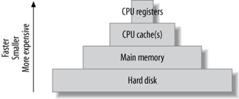
Figure 9-1. The cache hierarchy
Every level in this cache hierarchy is best used to cache “hot” data so it can be accessed more quickly, usually using heuristics such as “recently used data is likely to be used again soon” and “data that’s near recently used data is likely to be used soon.” These heuristics work because of spatial and temporal locality of reference.
From the programmer’s point of view, CPU registers and caches are transparent and architecture-specific. It is the compiler’s and CPU’s job to manage these. However, programmers are very conscious of the difference between main memory and the hard disk, and programs usually treat these very differently.[128]
This is especially true of database servers, whose behavior often goes against the predictions made by the heuristics we just mentioned. A well-designed database cache (such as the InnoDB buffer pool) is usually more efficient than an operating system’s cache, which is tuned for general-purpose tasks. The database cache has much more knowledge about its data needs, and it has special-purpose logic (write ordering, for example) that helps meet those needs. Also, a system call is not required to access the data in the database cache.
These special-purpose cache requirements are why you’ll have to balance your cache hierarchy to suit the particular access patterns of a database server. Because the registers and on-chip caches are not user-configurable, memory and the storage are the only things you can change.
Random Versus Sequential I/O
Database servers use both sequential and random I/O, and random I/O benefits the most from caching. You can convince yourself of this by thinking about a typical mixed workload, with some balance of single-row lookups and multirow range scans. The typical pattern is for the “hot” data to be randomly distributed; caching this data will therefore help avoid expensive disk seeks. In contrast, sequential reads generally go through the data only once, so it’s useless to cache it unless it fits completely in memory.
Another reason sequential reads don’t benefit much from caching is because they are faster than random reads. There are two reasons for this:
Sequential I/O is faster than random I/O.
Sequential operations are performed faster than random operations, both in memory and on disk. Suppose your disks can do 100 random I/O operations per second and can read 50 MB per second sequentially (that’s roughly what a consumer-grade disk can achieve today). If you have 100-byte rows, that’s 100 rows per second randomly, versus 500,000 rows per second sequentially—a difference of 5,000 times, or several orders of magnitude. Thus, the random I/O benefits more from caching in this scenario.
Accessing in-memory rows sequentially is also faster than accessing in-memory rows randomly. Today’s memory chips can typically access about 250,000 100-byte rows per second randomly, and 5 million per second sequentially. Note that random accesses are some 2,500 times faster in memory than on disk, while sequential accesses are only 10 times faster in memory.
Storage engines can perform sequential reads faster than random reads.
A random read generally means that the storage engine must perform index operations. (There are exceptions to this rule, but it’s true for InnoDB and MyISAM.) That usually requires navigating a B-Tree data structure and comparing values to other values. In contrast, sequential reads generally require traversing a simpler data structure, such as a linked list. That’s a lot less work, so again, sequential reads are faster.
Finally, random reads are typically executed to find individual rows, but the read isn’t just one row—it is a whole page of data, most of which isn’t needed. That’s a lot of wasted work. A sequential read, on the other hand, typically happens when you want all of the rows on the page, so it’s much more cost-effective.
As a result, you can save work by caching sequential reads, but you can save much more work by caching random reads instead. In other words, adding memory is the best solution for random-read I/O problems if you can afford it.
Caching, Reads, and Writes
If you have enough memory, you can insulate the disk from read requests completely. If all your data fits in memory, every read will be a cache hit once the server’s caches are warmed up. There will still be logical reads, but no physical reads. Writes are a different matter, though. A write can be performed in memory just as a read can, but sooner or later it has to be written to the disk so it’s permanent. In other words, a cache can delay writes, but caching cannot eliminate writes as it can reads.
In fact, in addition to allowing writes to be delayed, caching can permit them to be grouped together in two important ways:
Many writes, one flush
A single piece of data can be changed many times in memory without all of the new values being written to disk. When the data is eventually flushed to disk, all the modifications that happened since the last physical write are made permanent. For example, many statements could update an in-memory counter. If the counter is incremented 100 times and then written to disk, 100 modifications have been grouped into one write.
I/O merging
Many different pieces of data can be modified in memory and the modifications can be collected together, so the physical writes can be performed as a single disk operation.
This is why many transactional systems use a write-ahead logging strategy. Write-ahead logging lets them make changes to the pages in memory without flushing the changes to disk, which usually involves random I/O and is very slow. Instead, they write a record of the changes to a sequential log file, which is much faster. A background thread can flush the modified pages to disk later; when it does, it can optimize the writes.
Writes benefit greatly from buffering, because it converts random I/O into more sequential I/O. Asynchronous (buffered) writes are typically handled by the operating system and are batched so they can be flushed to disk more optimally. Synchronous (unbuffered) writes have to be written to disk before they finish. That’s why they benefit from buffering in a RAID controller’s battery-backed write-back cache (we discuss RAID a bit later).
What’s Your Working Set?
Every application has a “working set” of data—that is, the data that it really needs to do its work. A lot of databases also have plenty of data that’s not in the working set. You can imagine the database as a desk with filing drawers. The working set consists of the papers you need to have on the desktop to get your work done. The desktop is main memory in this analogy, while the filing drawers are the hard disks.
Just as you don’t need to have every piece of paper on the desktop to get your work done, you don’t need the whole database to fit in memory for optimal performance—just the working set.
The working set’s size varies greatly depending on the application. For some applications the working set might be 1% of the total data size, while for others it could be close to 100%. When the working set doesn’t fit in memory, the database server will have to shuffle data between the disk and memory to get its work done. This is why a memory shortage might look like an I/O problem. Sometimes there’s no way you can fit your entire working set in memory, and sometimes you don’t actually want to (for example, if your application needs a lot of sequential I/O). Your application architecture can change a lot depending on whether you can fit the working set in memory.
The working set can be defined as a time-based percentile. For example, the 95th percentile one-hour working set is the set of pages that the database uses during one hour, except for the 5% of pages that are least frequently used. A percentile is the most useful way to think about this, because you might need to access only 1% of your data every hour, but over a 24-hour period that might add up to around 20% of the distinct pages in the whole database. It might be more intuitive to think of the working set in terms of how much data you need to have cached, so your workload is mostly CPU-bound. If you can’t cache enough data, your working set doesn’t fit in memory.
You should think about the working set in terms of the most frequently used set of pages, not the most frequently read or written set of pages. This means that determining the working set requires instrumentation inside the application; you cannot just look at external usage such as I/O accesses, because I/O to the pages is not the same thing as logical access to the pages. MySQL might read a page into memory and then access it millions of times, but you’ll see only one I/O operation if you’re looking at strace, for example. The lack of instrumentation needed for determining the working set is probably the biggest reason that there isn’t a lot of research into this topic.
The working set consists of both data and indexes, and you should count it in cache units. A cache unit is the smallest unit of data that the storage engine works with.
The size of the cache unit varies between storage engines, and therefore so does the size of the working set. For example, InnoDB works in pages of 16 KB by default. If you do a single-row lookup and InnoDB has to go to disk to get it, it’ll read the entire page containing that row into the buffer pool and cache it there. This can be wasteful. Suppose you have 100-byte rows that you access randomly. InnoDB will use a lot of extra memory in the buffer pool for these rows, because it will have to read and cache a complete 16 KB page for each row. Because the working set includes indexes too, InnoDB will also read and cache the parts of the index tree it needed to find the row. InnoDB’s index pages are also 16 KB in size, which means it might have to store a total of 32 KB (or more, depending on how deep the index tree is) to access a single 100-byte row. The cache unit is, therefore, another reason why well-chosen clustered indexes are so important in InnoDB. Clustered indexes not only let you optimize disk accesses but also help you keep related data on the same pages, so you can fit more of your working set in your cache.
Finding an Effective Memory-to-Disk Ratio
A good memory-to-disk ratio is best discovered by experimentation and/or benchmarking. If you can fit everything into memory, you’re done—there’s no need to think about it further. But most of the time you can’t, so you have to benchmark with a subset of your data and see what happens. What you’re aiming for is an acceptable cache miss rate. A cache miss is when your queries request some data that’s not cached in main memory, and the server has to get it from disk.
The cache miss rate really governs how much of your CPU is used, so the best way to assess your cache miss rate is to look at your CPU usage. For example, if your CPU is used 99% of the time and waiting for I/O 1% of the time, your cache miss rate is good.
Let’s consider how your working set influences your cache miss rate. It’s important to realize that your working set isn’t just a single number: it’s a statistical distribution, and your cache miss rate is nonlinear with regard to the distribution. For example, if you have 10 GB of memory and you’re getting a 10% cache miss rate, you might think you just need to add 11% more memory[129] to reduce the cache miss rate to zero. But in reality, inefficiencies such as the size of the cache unit might mean you’d theoretically need 50 GB of memory just to get a 1% miss rate. And even with a perfect cache unit match, the theoretical prediction can be wrong: factors such as data access patterns can complicate things even more. A 1% cache miss rate might require 500 GB of memory, depending on your workload!
It’s easy to get sidetracked focusing on optimizing something that might not give you much benefit. For example, a 10% miss rate might result in 80% CPU usage, which is already pretty good. Suppose you add memory and are able to get the cache miss rate down to 5%. As a gross oversimplification, you’ll be delivering approximately another 6% data to the CPUs. Making another gross oversimplification, we could say that you’ve increased your CPU usage to 84.8%. However, this isn’t a very big win, considering how much memory you might have purchased to get that result. And in reality, because of the differences between the speed of memory and disk accesses, what the CPU is really doing with the data, and many other factors, lowering the cache miss rate by 5% might not change your CPU usage much at all.
This is why we said you should strive for an acceptable cache miss rate, not a zero cache miss rate. There’s no single number you should target, because what’s considered “acceptable” will depend on your application and your workload. Some applications might do very well with a 1% cache miss rate, while others really need a rate as low as 0.01% to perform well. (A “good cache miss rate” is a fuzzy concept, and the fact that there are many ways to count the miss rate further complicates matters.)
The best memory-to-disk ratio also depends on other components in your system. Suppose you have a system with 16 GB of memory, 20 GB of data, and lots of unused disk space. The system is performing nicely at 80% CPU usage. If you wish to place twice as much data on this system and maintain the same level of performance, you might think you can just double the number of CPUs and the amount of memory. However, even if every component in the system scaled perfectly with the increased load (an unrealistic assumption), this probably wouldn’t work. The system with 20 GB of data is likely to be using more than 50% of some component’s capacity—for example, it might already be performing 80% of its maximum number of I/O operations per second. And queueing inside the system is nonlinear, too. The server won’t be able to handle twice as much load. Thus, the best memory-to-disk ratio depends on the system’s weakest component.
Choosing Hard Disks
If you can’t fit enough data in memory—for example, if you estimate you would need 500 GB of memory to fully load your CPUs with your current I/O system—you should consider a more powerful I/O subsystem, sometimes even at the expense of memory. And you should design your application to handle I/O wait.
This might seem counterintuitive. After all, we just said that more memory can ease the pressure on your I/O subsystem and reduce I/O waits. Why would you want to beef up the I/O subsystem if adding memory could solve the problem? The answer lies in the balance between the factors involved, such as the number of reads versus writes, the size of each I/O operation, and how many such operations happen every second. For example, if you need fast log writes, you can’t shield the disk from these writes by increasing the amount of available memory. In this case, it might be a better idea to invest in a high-performance I/O system with a battery-backed write cache, or solid-state storage.
As a brief refresher, reading data from a conventional hard disk is a three-step process:
1. Move the read head to the right position on the disk’s surface.
2. Wait for the disk to rotate, so the desired data is under the read head.
3. Wait for the disk to rotate all the desired data past the read head.
How quickly the disk can perform these operations can be condensed to two numbers: access time (steps 1 and 2 combined) and transfer speed. These two numbers also determine latency and throughput. Whether you need fast access times or fast transfer speeds—or a mixture of the two—depends on the kinds of queries you’re running. In terms of total time needed to complete a disk read, small random lookups are dominated by steps 1 and 2, while big sequential reads are dominated by step 3.
Several other factors can also influence the choice of disk, and which are important will depend on your application. Let’s imagine you’re choosing disks for an online application such as a popular news site, which does a lot of small, random reads. You might consider the following factors:
Storage capacity
This is rarely an issue for online applications, because today’s disks are usually more than big enough. If they’re not, combining smaller disks with RAID is standard practice.[130]
Transfer speed
Modern disks can usually transfer data very quickly, as we saw earlier. Exactly how quickly depends mostly on the spindle rotation speed and how densely the data is stored on the disk’s surface, plus the limitations of the interface with the host system (many modern disks can read data faster than the interface can transfer it). Regardless, transfer speed is usually not a limiting factor for online applications, because they generally do a lot of small, random lookups.
Access time
This is usually the dominating factor in how fast your random lookups will perform, so you should look for fast access time.
Spindle rotation speed
Common rotation speeds today are 7,200 RPM, 10,000 RPM, and 15,000 RPM. The rotation speed contributes quite a bit to the speed of both random lookups and sequential scans.
Physical size
All other things being equal, the physical size of the disk makes a difference, too: the smaller the disk is, the less time it takes to move the read head. Server-grade 2.5-inch disks are often faster than their larger cousins. They also use less power, and you can usually fit more of them into the chassis.
Just as with CPUs, how MySQL scales to multiple disks depends on the storage engine and the workload. InnoDB scales well to many hard drives. However, MyISAM’s table locks limit its write scalability, so a write-heavy workload on MyISAM probably won’t benefit much from having many drives. Operating system buffering and parallel background writes help somewhat, but MyISAM’s write scalability is inherently more limited than InnoDB’s.
As with CPUs, more disks is not always better. Some applications that demand low latency need faster drives, not more drives. For example, replication usually performs better with faster drives, because updates on a replica are single-threaded.
[128] However, programs might rely on the operating system to cache in memory a lot of data that’s conceptually “on disk.” This is what MyISAM does, for example. It treats the data files as disk-resident, and lets the operating system take care of caching the disk’s data to make it faster.
[129] The right number is 11%, not 10%. A 10% miss rate is a 90% hit rate, so you need to divide 10 GB by 90%, which is 11.111 GB.
[130] Interestingly, some people deliberately buy larger-capacity disks, then use only 20–30% of their capacity. This increases the data locality and decreases the seek time, which can sometimes justify the higher price.
Solid-State Storage
Solid-state (flash) storage is actually a 30-year-old technology, but it’s become a hot new thing as a new generation of devices have evolved over the last few years. Solid-state storage has now become sufficiently cheap and mature that it is in widespread use, and it will probably replace traditional hard drives for many purposes in the near future.
Solid-state storage devices use nonvolatile flash memory chips composed of cells, instead of magnetic platters. They’re also called NVRAM, or nonvolatile random access memory. They have no moving parts, which makes them behave very differently from hard drives. We will explore the differences in detail.
The current technologies of interest to MySQL users can be divided into two major categories: SSDs (solid-state drives) and PCIe cards. SSDs emulate standard hard drives by implementing the SATA (Serial Advanced Technology Attachment) interface, so they are drop-in replacements for the hard drive that’s in your server now and can fit into the existing slots in the chassis. PCIe cards use special operating system drivers that present the storage as a block device. PCIe and SSD devices are sometimes casually referred to as simply SSDs.
Here’s a quick summary of flash performance. High-quality flash devices have:
§ Much better random read and write performance compared to hard drives. Flash devices are usually slightly better at reads than writes.
§ Better sequential read and write performance than hard drives. However, it’s not as dramatic an improvement as that of random I/O, because hard drives are much slower at random I/O than they are at sequential I/O. Entry-level SSDs can actually be slower than conventional drives here.
§ Much better support for concurrency than hard drives. Flash devices can support many more concurrent operations, and in fact, they don’t really achieve their top throughput until you have lots of concurrency.
The most important things are the improvements in random I/O and concurrency. Flash memory gives you very good random I/O performance at high concurrency, which is exactly what properly normalized databases need. One of the most common reasons for denormalizing a schema is to avoid random I/O and make it possible for sequential I/O to serve the queries.
As a result, we believe that solid-state storage is going to change RDBMS technology fundamentally in the future. The current generation of RDBMS technology has undergone decades of optimizations for spindle-based storage. The same maturity and depth of research and engineering don’t quite exist yet for solid-state storage.[131]
An Overview of Flash Memory
Hard drives with spinning platters and oscillating heads have inherent limitations and characteristics that are consequences of the physics involved. The same is true of solid-state storage, which is built on top of flash memory. Don’t get the idea that solid-state storage is simple. It’s actually more complex than a hard drive in some ways. The limitations of the flash memory are actually pretty severe and hard to overcome, so the typical solid-state device has an intricate architecture with lots of abstractions, caching, and proprietary “magic.”
The most important characteristic of flash memory is that it can be read many times rapidly, and in small units, but writes are much more challenging. You can’t rewrite a cell[132] without a special erase operation, and you can erase only in large blocks—for example, 512 KB. The erase cycle is slow, and eventually wears out the block. The number of erase cycles a block can tolerate depends on the underlying technology it uses; more about this later.
The limitations on writes are the reason for the complexity of solid-state storage. This is why some devices provide stable, consistent performance and others don’t. The magic is all in the proprietary firmware, drivers, and other bits and pieces that make a solid-state device run. To make writes perform well and avoid wearing out the blocks of flash memory prematurely, the device must be able to relocate pages and perform garbage collection and so-called wear leveling. The term write amplification is used to describe the additional writes caused by moving data from place to place, writing data and metadata multiple times due to partial block writes. If you’re interested, Wikipedia’s article on write amplification is a good place to learn more.
Garbage collection is important to understand. In order to keep some blocks fresh and ready for new writes, the device reclaims blocks. This requires some free space on the device. Either the device will have some reserved space internally that you can’t see, or you will need to reserve space yourself by not filling it up all the way—this varies from device to device. Either way, as the device fills up, the garbage collector has to work harder to keep some blocks clean, so the write amplification factor increases.
As a result, many devices get slower as they fill up. How much slower is different for every vendor and model, and depends on the device’s architecture. Some devices are designed for high performance even when they are pretty full, but in general, a 100 GB file will perform differently on a 160 GB SSD than on a 320 GB SSD. The slowdown is caused by having to wait for erases to complete when there are no free blocks. A write to a free block takes a couple of hundred microseconds, but an erase is much slower—typically a few milliseconds.
Flash Technologies
There are two major types of flash devices, and when you’re considering a flash storage purchase, it’s important to understand the differences. The two types are single-level cell (SLC) and multi-level cell (MLC).
SLC stores a single bit of data per cell: it can be either a 0 or a 1. SLC is relatively expensive, but it is very fast and durable, with a lifetime of up to 100,000 write cycles depending on the vendor and model. This might not sound like much, but in reality a good SLC device ought to last about 20 years or so, and is said to be more durable and reliable than the controller on which the card is mounted. On the downside, the storage density is relatively low, so you can’t get as much storage space per device.
MLC stores two bits per cell, and three-bit devices are entering the market. This makes it possible to get much higher storage density (larger capacities) with MLC devices. The cost is lower, but so is the speed and durability. A good MLC device might be rated for around 10,000 write cycles.
You can purchase both types of flash devices on the mass market, and there is active development and competition between them. At present, SLC still holds the reputation for being the “enterprise” server-grade storage solution, and MLC is usually regarded as consumer-grade, for use in laptops and cameras and so on. However, this is changing, and there is an emerging category of so-called enterprise MLC (eMLC) storage.
The development of MLC technology is interesting and bears close watching if you’re considering purchasing flash storage. MLC is very complex, with a lot of important factors that contribute to a device’s quality and performance. Any given chip by itself is not durable, with a relatively short lifetime and a high probability of errors that must be corrected. As the market moves to even smaller, higher-density chips where the cells can store three bits, the individual chips become even less reliable and more error-prone.
However, this isn’t an insurmountable engineering problem. Vendors are building devices with lots and lots of spare capacity that’s hidden from you, so there is internal redundancy. There are rumors that some devices might have up to twice as much storage as their rated size, although flash vendors guard their trade secrets very closely. Another way to make MLC chips more durable is through the firmware logic. The algorithms for wear leveling and remapping are very important.
Longevity therefore depends on the true capacity, the firmware logic, and so on—it is ultimately vendor-specific. We’ve heard reports of devices being destroyed in a couple of weeks of intensive use!
As a result, the most critical aspects of an MLC device are the algorithms and intelligence built into it. It’s much harder to build a good MLC device than an SLC device, but it is possible. With great engineering and increases in capacity and density, some of the best vendors are offering devices that are worthy of the eMLC label. This is definitely an area where you’ll want to keep track of progress over time; this book’s advice on MLC versus SLC is likely to become outdated pretty quickly.
HOW LONG WILL YOUR DEVICE LAST?
Virident guarantees that its FlashMax 1.4 TB MLC device will last for 15 PB (petabytes) of writes, but that’s at the flash level, and user-visible writes are amplified. We ran a little experiment to discover the write amplification factor for a specific workload.
We created a 500 GB dataset and ran the tpcc-mysql benchmark on it for an hour. During this hour /proc/diskstats reported 984 GB of writes, and the Virident configuration utility showed 1,125GB of writes at the flash level, for a write amplification factor of 1.14. Remember, this will be higher if more space is consumed on the device, and it varies based on whether the writes are sequential or random.
At this rate, if we ran the benchmark continuously for a year and a half, we’d wear out the device. Of course, most real workloads are nowhere close to this write-intensive, so the card should last many years in practical usage. The point of this sidebar is not to say that the device will wear out quickly—it is to say that the write amplification factor is hard to predict, and you need to check your device under your workload to see how it behaves.
Size also matters a lot for longevity, as we’ve mentioned. Bigger devices should last significantly longer, which is why MLC is getting more popular—we’re seeing large enough capacities these days for the longevity to be reasonable.
Benchmarking Flash Storage
Benchmarking flash storage is complicated and difficult. There are many ways to do it wrong, and it requires device-specific knowledge, as well as great care and patience, to do it right.
Flash devices have a three-stage pattern that we call the A-B-C performance characteristics. They start out running fast (stage A), and then the garbage collector starts to work. This causes a period during which the device is transitioning to a steady state (stage B), and finally the device enters a steady state (stage C). All of the devices we’ve tested have this characteristic pattern.
Of course, what you’re interested in is the performance in stage C, so your benchmarks need to measure only that portion of the run. This means that the benchmark needs to be more than just a benchmark: it needs to be a warmup workload followed by a benchmark. Defining where the warmup ends and the benchmark begins can be tricky, though.
Devices, filesystems, and operating systems vary in their support for the TRIM command, which marks space as ready to reuse. Sometimes the device will TRIM when you delete all of the files. If that happens between runs of the benchmark, the device will reset to stage A, and you’ll have to cycle it through stages A and B between runs. Another factor is the differing performance when the device is more or less filled up. A repeatable benchmark has to account for all of these factors.
As a result of the above complexities, vendor benchmarks and specifications are a minefield for the unwary, even when they’re reported faithfully and with good intentions. You typically get four numbers from vendors. Here’s an example of a device’s specifications:
1. The device can read up to 520 MB/s.
2. The device can write up to 480 MB/s.
3. The device can perform sustained writes up to 420 MB/s.
4. The device can perform 70,000 random 4 KB writes per second.
If you cross-check those numbers, you will notice that the peak IOPS (input/output operations per second) of 70,000 random 4 KB writes per second is only about 274 MB/s, which is a lot less than the peak write bandwidths listed in points 2 and 3. This is because the peak write bandwidth is achieved with large block sizes such as 64 KB or 128 KB, and the peak IOPS is achieved with small block sizes.
Most applications don’t write in such large blocks. InnoDB typically writes a combination of 16 KB blocks and 512-byte blocks. As a result, you should really expect only 274 MB/s of write bandwidth from this device—and that’s in stage A, before the garbage collector kicks in and the device reaches its steady-state long-term performance levels!
You can find current benchmarks of MySQL and raw file I/O workloads on solid-state devices at our blogs, http://www.ssdperformanceblog.com and http://www.mysqlperformanceblog.com.
Solid-State Drives (SSDs)
SSDs emulate SATA hard drives. This is a compatibility feature: a replacement for a SATA drive doesn’t require any special drivers or interconnects.
Intel X-25E drives are probably the most common SSDs we see used in servers today, but there are lots of other options. The X-25E is sold for the “enterprise” market, but there is also the X-25M, which has MLC storage and is intended for the mass market of laptop users and so forth. Intel also sells the 320 series, which a lot of people are using as well. Again, this is just one vendor—there are many, and by the time this book goes to print, some of what we’ve written about SSDs will likely already be outdated.
The good thing about SSDs is that they are readily available in lots of brands and models, they’re relatively cheap, and they’re a lot faster than hard drives. The biggest downside is that they’re not always as reliable as hard drives, depending on the brand and model. Until recently, most devices didn’t have an onboard battery, but most devices do have a write cache to buffer writes. This write cache isn’t durable without a battery to back it, but it can’t be disabled without greatly increasing the write load on the underlying flash storage. So, if you disable your drive’s cache to get really durable storage, you will wear the device out faster, and in some cases this will void the warranty.
Some manufacturers don’t exactly rush to inform people about this characteristic of the SSDs they sell, and they guard details such as the internal architecture of the devices pretty jealously. Whether there is a battery or capacitor to keep the write cache’s data safe in case of a power failure is usually an open question. In some cases the drive will accept a command to disable the cache, but ignore it. So you really won’t know whether your drive is durable unless you do crash testing. We crash-tested some drives and found varying results. These days some drives ship with a capacitor to protect the cache, making it durable, but in general, if your drive doesn’t brag that it has a battery or capacitor, then it doesn’t. This means it isn’t durable in case of power outages, so you’ll get data corruption, possibly without knowing it. A capacitor or battery is a feature you should definitely look for in SSDs.
You generally get what you pay for with SSDs. The challenges of the underlying technology aren’t easy to solve. Lots of manufacturers make drives that fail shockingly quickly under load, or don’t provide consistent performance. Some low-end manufacturers have a habit of releasing a new generation of drives every time you turn around, and claiming that they’ve solved all the problems of the older generation. This tends to be untrue, of course. The “enterprise-grade” devices are usually worth the price if you care about reliability and consistently high performance.
Using RAID with SSDs
We recommend that you use RAID (Redundant Array of Inexpensive Disks) with SATA SSDs. They are simply not reliable enough to trust a single drive with your data.
Many older RAID controllers weren’t SSD-ready. They assumed that they were managing spindle-based hard drives, and they did things like buffering and reordering writes, assuming that it would be more efficient. This was just wasted work and added latency, because the logical locations that the SSD exposes are mapped to arbitrary locations in the underlying flash memory. The situation is a bit better today. Some RAID controllers have a letter at the end of their model numbers, indicating that they are SSD-ready. For example, the Adaptec controllers use a Z for this purpose.
Even flash-ready controllers are not really flash-ready, however. For example, Vadim benchmarked an Adaptec 5805Z controller with a variety of drives in RAID 10, using a 500 GB file and a concurrency of 16. The results were terrible: the 95th percentile latency for random writes was in the double-digit milliseconds, and in the worst case, it was over a second.[133] (You should expect sub-millisecond writes.)
This specific comparison was for a customer who wanted to see whether Micron SSDs would be better than 64 GB Intel SSDs, which they already used in the same configuration. When we benchmarked the Intel drives, we found the same performance characteristics. So we tried some other configurations of drives, with and without a SAS expander, to see what would happen. Table 9-1 shows the results.
Table 9-1. Benchmarks with SSDs on an Adaptec RAID controller
|
Drives |
Brand |
Size |
SAS expander |
Random read |
Random write |
|
34 |
Intel |
64 GB |
Yes |
310 MB/s |
130 MB/s |
|
14 |
Intel |
64 GB |
Yes |
305 MB/s |
145 MB/s |
|
24 |
Micron |
50 GB |
No |
350 MB/s |
120 MB/s |
|
34 |
Intel |
50 GB |
No |
350 MB/s |
180 MB/s |
None of these results approached what we should expect from so many drives. In general, the RAID controller was giving us the performance we’d expect from six or eight drives, not dozens. The RAID controller was simply saturated. The point of this story is that you should benchmark carefully before investing heavily in hardware—the results might be quite different from your expectations.
PCIe Storage Devices
In contrast to SATA SSDs, PCIe devices don’t try to emulate hard drives. This is a good thing: the interface between the server and the hard drives isn’t capable of handling the full performance of flash. The SAS/SATA interconnect has lower bandwidth than PCIe, so PCIe is a better choice for high performance. PCIe devices also have much lower latency, because they are physically closer to the CPUs.
Nothing matches the performance you can get from PCIe devices. The downside is that they’re relatively expensive.
All of the models we’re familiar with require a special driver to create a block device that the operating system sees as a hard drive. They use a mixture of strategies for their wear leveling and other logic; some of them use the host system’s CPU and memory, and some have onboard logic controllers and RAM. In many cases the host system has plentiful CPU and RAM resources, so using them is actually a more cost-effective strategy than buying a card that has its own.
We don’t recommend RAID with PCIe devices. They’re too expensive to use with RAID, and most devices have their own onboard RAID anyway. We don’t really know how likely the controller is to fail, but the vendors say that their controllers should be as good as network cards or RAID controllers in general, and this seems likely to be true. In other words, the mean time between failures (MTBF) for these devices is likely to be similar to the motherboard, so using RAID with the devices would just add a lot of cost without much benefit.
There are several vendors making PCIe flash cards. The most popular brands among MySQL users are Fusion-io and Virident, but vendors such as Texas Memory Systems, STEC, and OCZ also have offerings. Both SLC and MLC cards are available.
Other Types of Solid-State Storage
In addition to SSDs and PCIe devices, there are other options from companies such as Violin Memory, SandForce, and Texas Memory Systems. These companies provide large boxes full of flash memory that are essentially flash SANs, with tens of terabytes of storage. They’re used mostly for large-scale data center storage consolidation. They’re very expensive and very high-performance. We know of some people who use them, and we have measured their performance in some cases. They provide very decent latency despite the network round-trip time—for example, less than four milliseconds of latency over NFS.
These aren’t really a good fit for the general MySQL market, though. They’re more targeted towards other databases, such as Oracle, which can use them for shared-storage clustering. MySQL can’t take advantage of such powerful storage at such a large scale, in general, as it doesn’t typically run well with databases in the tens of terabytes—MySQL’s answer to such a large database is to shard and scale out horizontally in a shared-nothing architecture.
Specialized solutions might be able to use these large storage devices, though—Infobright might be a candidate, for example. ScaleDB can be deployed in a shared-storage architecture, but we haven’t seen it in production, so we don’t know how well it might work.
When Should You Use Flash?
The most obvious use case for solid-state storage is any workload that has a lot of random I/O. Random I/O is usually caused by the data being larger than the server’s memory. With standard hard drives, you’re limited by rotation speed and seek latency. Flash devices can ease the pain significantly.
Of course, sometimes you can simply buy more RAM so the random workload will fit into memory, and the I/O goes away. But when you can’t buy enough RAM, flash can help. Another problem that you can’t always solve with RAM is that of a high-throughput write workload. Adding memory will help reduce the write workload that reaches the disks, because more memory creates more opportunities to buffer and combine writes. This allows you to convert a random write workload into a more sequential one. However, this doesn’t work infinitely, and some transactional or insert-heavy workloads don’t benefit from this approach anyway. Flash storage can help here, too.
Single-threaded workloads are another characteristic scenario where flash can potentially help. When a workload is single-threaded it is very sensitive to latency, and the lower latency of solid-state storage makes a big difference. In contrast, multi-threaded workloads can often simply be parallelized more heavily to get more throughput. MySQL replication is the obvious example of a single-threaded workload that benefits a lot from reduced latency. Using flash storage on replicas can often improve their performance significantly when they are having trouble keeping up with the master.
Flash is also great for server consolidation, especially in the PCIe form factor. We’ve seen opportunities to consolidate many server instances onto a single physical server—sometimes up to a 10- or 15-fold consolidation is possible. See Chapter 11 for more on this topic.
Flash isn’t always the answer, though. A good example is for sequential write workloads such as the InnoDB log files. Flash doesn’t offer much of a cost-to-performance advantage in this scenario, because it’s not much faster at sequential writes than standard hard drives are. Such workloads are also high-throughput, which will wear out the device faster. It’s often a better idea to store your log files on standard hard drives, with a RAID controller that has a battery-backed write cache.
And sometimes the answer lies in the memory-to-disk ratio, not just in the disk. If you can buy enough RAM to cache your workload, you may find this cheaper and more effective than purchasing a flash storage device.
Using Flashcache
Although there are many opportunities to make tradeoffs between flash storage, hard disks, and RAM, these don’t have to be treated as single-component tiers in the storage hierarchy. Sometimes it makes sense to use a combination of disk and memory technologies, and that’s what Flashcache does.
Flashcache is one implementation of a technique you can find used in many systems, such as Oracle Database, the ZFS filesystem, and even many modern hard drives and RAID controllers. Much of the following discussion applies broadly, but to keep things concrete we’ll focus only on Flashcache, because it is vendor-and filesystem-agnostic.
Flashcache is a Linux kernel module that uses the Linux device mapper. It creates an intermediate layer in the memory hierarchy, between RAM and the disk. It is one of the open source technologies created by Facebook and is used to help optimize Facebook’s hardware for its database workload.
Flashcache creates a block device, which can be partitioned and used to create a filesystem like any other. The trick is that this block device is backed by both flash and disk storage. The flash device is used as an intelligent cache for both reads and writes. The virtual block device is much larger than the flash device, but that’s okay, because the disk is considered to be the ultimate repository for the data. The flash device is just there to buffer writes and to effectively extend the server’s memory size for caching reads.
How good is performance? Flashcache seems to have relatively high kernel overhead. (The device mapper doesn’t seem to be as efficient as it should be, but we haven’t probed deeply to find out why.) However, even though it seems that Flashcache could theoretically be more efficient, and the ultimate performance is not as good as the performance of the underlying flash storage, it’s still a lot faster than disks. So it might be worthwhile to consider.
We evaluated Flashcache’s performance in a series of hundreds of benchmarks, and we found that it’s rather difficult to test meaningfully on an artificial workload. We concluded that it’s not clear how beneficial Flashcache is for write workloads in general, but for read workloads it can be very helpful. This matches the use case for which it was designed: servers that are heavily I/O-bound on reads, with a much larger working set than the memory size.
In addition to lab testing, we have some experience with Flashcache in production workloads. One case of a four-terabyte database comes to mind. This database suffered greatly from replication lag. We modified the system by adding a Virident PCIe card with half a terabyte of storage. Then we installed Flashcache and used the PCIe card as the flash portion of the device. This doubled replication speed.
The Flashcache use case is most economical when the flash card is pretty full, so it’s important to have a card whose performance doesn’t degrade much when it fills up. That’s why we chose the Virident card.
Flashcache really is a cache, so it has to warm up just like any other cache. This warmup period can be extremely long, though. For example, in the case we just mentioned, Flashcache required a week to warm up and really help accelerate the workload.
Should you use Flashcache? Your mileage will vary, so we think it’s a good idea to get expert advice on this point if you feel uncertain. It’s complex to understand the mechanics of Flashcache, and how they impact your database’s working set size and the (at least) three layers of storage underneath the database:
§ First there’s the InnoDB buffer pool, whose size relative to the working set size determines one cache miss rate. Hits from this cache are very fast, and the response time is very uniform.
§ Misses from the buffer pool propagate down to the Flashcache device, which has a complex distribution of response times. Flashcache’s cache miss rate is determined by the working set size and the size of the flash device that backs it. Hits from this cache are a lot faster than disk retrievals.
§ Misses from Flashcache’s cache propagate down to the disks, which have a fairly uniform distribution of response times.
There might be more layers beyond that: your SAN or your RAID controller cache, for example.
Here’s a thought experiment that illustrates how these layers interact. It’s clear that the response times from a Flashcache device will not be as stable or fast as they would be from the flash device alone. But imagine that you have a terabyte of data, and 100 GB of this data receives 99% of the I/O operations over a long period of time. That is, the long-term 99th percentile working set size is 100 GB.
Now suppose that we have the following storage devices: a large RAID volume that can perform 1,000 IOPS, and a much smaller flash device that can perform 100,000 IOPS. The flash device is not big enough to store all of the data—let’s pretend it is 128 GB—so using flash alone isn’t an option. If we use the flash device for Flashcache, we can expect cache hits to be much faster than disk retrievals, but slower than the responses from flash device itself. Let’s stick with round numbers and say that 90% of the requests to the Flashcache device can be served at a rate equivalent to 50,000 IOPS.
What is the outcome of this thought experiment? There are two major points:
1. Our system provides a lot better performance with Flashcache than without it, because most of the page accesses that are cache misses in the buffer pool are served from the flash card at a very high speed relative to disk accesses. (The 99th percentile working set fits entirely into the flash card.)
2. The 90% hit rate at the Flashcache device means there is a 10% miss rate. Because the underlying disks can serve only 1,000 IOPS, the most we can expect to push to the Flashcache device is 10,000 IOPS. To understand why this is true, imagine what would happen if we requested more than that: with 10% of the I/O operations missing the cache and falling through to the RAID volume, we’d be requesting more than 1,000 IOPS of the RAID volume, and we know it can’t handle that. As a result, even though Flashcache is slower than the flash card, the system as a whole is still limited by the RAID volume, not the flash card or Flashcache.
In the final analysis, whether Flashcache is right for you is a complex decision that will involve lots of factors. In general, it seems best suited to heavily I/O-bound read-mostly workloads whose working set size is much too large to be optimized economically with memory.
Optimizing MySQL for Solid-State Storage
If you’re running MySQL on flash, there are some configuration parameters that can provide better performance. The default configuration of InnoDB, in particular, is tailored to hard drives, not solid-state drives. Not all versions of InnoDB provide the same level of configurability. In particular, many of the improvements designed for flash have appeared first in Percona Server, although many of these have either already been reimplemented in Oracle’s version of InnoDB, or appear to be planned for future versions. Improvements include:
Increasing InnoDB’s I/O capacity
Flash supports much higher concurrency than conventional hard drives, so you can increase the number of read and write I/O threads to as high as 10 or 15 with good results. You can also increase the innodb_io_capacity option to between 2000 and 20000, depending on the IOPS your device can actually perform. This is especially necessary with the official InnoDB from Oracle, which has more internal algorithms that depend on this setting.
Making the InnoDB log files larger
Even with the improved recovery algorithms in recent versions of InnoDB, you don’t want your log files to be too large on hard drives, because the random I/O required for crash recovery is slow and can cause recovery to take a long time. Flash storage makes this much faster, so you can have larger InnoDB log files, which can help improve and stabilize performance. This is especially necessary with the official InnoDB from Oracle, which has trouble maintaining a consistent dirty page flush rate unless the log files are fairly large—4 GB or larger seems to be a good range on typical servers at the time of writing. Percona Server and MySQL 5.6 support log files larger than 4 GB.
Moving some files from flash to RAID
In addition to making the InnoDB log files larger, it can be a good idea to store the log files separately from the data files, placing them on a RAID controller with a battery-backed write cache instead of on the solid-state device. There are several reasons for this. One is that the type of I/O the log files receive isn’t much faster on flash devices than it is on such a RAID setup. InnoDB writes the log files sequentially in 512-byte units and never reads them except during crash recovery, when it reads them sequentially. It’s kind of wasteful to use your flash storage for this. It’s also a good idea to move these small writes to the RAID volume because very small writes increase the write amplification factor on flash devices, which can be a problem for some devices’ longevity. A mixture of large and small writes can also cause increased latency for some devices.
It’s also sometimes beneficial to move your binary log files to the RAID volume, for similar reasons; and you might consider moving your ibdata1 file, too. The ibdata1 file contains the doublewrite buffer and the insert buffer. The doublewrite buffer, in particular, gets a lot of repeated writes. In Percona Server, you can remove the doublewrite buffer from the ibdata1 file and store it in a separate file, which you can place on the RAID volume.
There’s another option, too: you can take advantage of Percona Server’s ability to write the transaction logs in 4-kilobyte blocks instead of 512-byte blocks. This can be more efficient for flash storage as well as for the server itself.
All of the above advice is rather hardware-specific, and your mileage may vary, so be sure you understand the factors involved—and test appropriately—before you make such a large change to your storage layout.
Disabling read-ahead
Readahead optimizes device access by noticing and predicting read patterns, and requesting data from the device when it believes that it will be needed in the future. There are actually two types of read-ahead in InnoDB, and in various circumstances we’ve found that performance problems can actually be caused by read-ahead and the way it works internally. The overhead is greater than the benefit in many cases, especially on flash storage, but we don’t have hard evidence or guidelines as to exactly how much you can improve performance by disabling read-ahead.
Oracle disabled so-called “random read-ahead” in the InnoDB plugin in MySQL 5.1, then reenabled it in MySQL 5.5 with a parameter to configure it. Percona Server lets you configure both random and linear read-ahead in older server versions as well.
Configuring the InnoDB flushing algorithm
The way that InnoDB decides when, how many, and which pages to flush is a highly complex topic to explore, and we don’t have room to discuss it in great detail here. This is also a subject of active research, and in fact several algorithms are available in various versions of InnoDB and MySQL.
The standard InnoDB’s algorithms don’t offer much configurability that is beneficial on flash storage, but if you’re using Percona XtraDB (included in Percona Server and MariaDB), we recommend setting the innodb_adaptive_checkpoint option to keep_average, instead of the default value of estimate. This will help ensure more consistent performance and avoid server stalls, because the estimate algorithm can stall on flash storage. We developed keep_average specifically for flash storage, because we realized that it’s possible to push as much I/O to the device as we want without causing a bottleneck and an ensuing stall.
In addition, we recommend setting innodb_flush_neighbor_pages to 0 on flash storage. This will prevent InnoDB from trying to find nearby dirty pages to flush together. The algorithm that performs this operation can cause large spikes of writes, high latency, and internal contention. It’s not necessary or beneficial on flash storage, because the neighboring pages can be flushed individually without impacting performance.
Potentially disabling the doublewrite buffer
Instead of moving the doublewrite buffer off the flash device, you can consider disabling it altogether. Some vendors claim that their devices support atomic 16 KB writes, which makes the doublewrite buffer redundant. You need to ensure that the entire storage system is configured to support atomic 16 KB writes, which generally requires O_DIRECT and the XFS filesystem.
We don’t have conclusive evidence that the claim of atomicity is true, but because of how flash storage works, we believe that the chance of partial page writes to the data files is greatly decreased. And the gains are much greater on flash devices than they are on conventional hard drives. Disabling the doublewrite buffer can improve MySQL’s overall performance on flash storage by a factor of 50% or so, so although we don’t know that it’s 100% safe, it’s something you can consider doing.
Restricting the insert buffer size
The insert buffer (or change buffer, in newer versions of InnoDB) is designed to reduce random I/O to nonunique secondary index pages that aren’t in memory when rows are updated. On hard drives, it can make a huge difference in reducing random I/O. For some workloads, the difference may reach nearly two orders of magnitude when the working set is much larger than memory. Letting the insert buffer grow large is very helpful in such cases.
However, this isn’t as necessary on flash storage. Random I/O is much faster on flash devices, so even if you disable the insert buffer completely, it doesn’t hurt as badly. You probably don’t want to disable it, though. It’s better to leave it enabled, because the I/O is only one part of the cost of updating index pages that aren’t in memory. The main thing to configure on flash devices is the maximum permitted size. You can restrict it to a relatively small size, instead of letting it grow huge; this can avoid consuming a lot of space on your device and help prevent the ibdata1 file from growing very large. At the time of writing you can’t configure the maximum size in standard InnoDB, but you can in Percona XtraDB, which is included in Percona Server and MariaDB. MySQL 5.6 will add a similar option, too.
In addition to the aforementioned configuration suggestions, some other optimizations have been proposed or discussed for flash storage. However, these are not all as clear-cut, so we will mention them but leave you to research their benefit for your specific case. The first is the InnoDB page size. We’ve found mixed results, so we don’t have a definite recommendation yet. The good news is that the page size is configurable without recompiling the server in Percona Server, and this will also be possible in MySQL 5.6. Previous versions of MySQL required you to recompile the server to use a different page size, so the general public has by far the most experience running with standard 16 KB pages. When the page size becomes easier for more people to experiment with, we expect a lot more testing with nonstandard sizes, and it’s likely that we’ll learn a great deal from this.
Another proposed optimization is alternative algorithms for InnoDB’s page checksums. When the storage system responds very quickly, the checksum computation can actually start to take a significant amount of time relative to the I/O operation, and for some people this has become the bottleneck instead of the I/O being the bottleneck. Our benchmarks haven’t shown repeatable results that are applicable to a broad spectrum of use cases, so your mileage may vary. Percona XtraDB permits you to change the checksum algorithm, and MySQL 5.6 will also have this capability.
You might have noticed that we’ve referred a lot to features and optimizations that aren’t available yet in standard InnoDB. We hope and believe that many of the improvements we’ve built into Percona Server and XtraDB will eventually become available to a wider audience. In the meantime, if you’re using the official MySQL distribution from Oracle, there are still steps you can take to optimize your server for flash storage. You should use innodb_file_per_table, and place the data directory on your flash device. Then move the ibdata1 and log files, and all other log files (binary logs, relay logs, etc.), to a RAID volume as discussed previously. This will concentrate the random I/O workload on your flash device and move as many of the write-heavy, sequentially written files off this device as possible, so you can save space on your flash device and reduce wear.
In addition, for all versions of the server, you should ensure that hyperthreading is enabled. It helps a lot when you use flash storage, because the disk is generally no longer the bottleneck, and tasks become more CPU-bound instead of being I/O-bound.
[131] Some companies claim that they’re starting with a clean slate, free of the fetters of the spindle-based past. Mild skepticism is warranted; solving RDBMS challenges is not easy.
[132] This is a simplification, but the details are not important here. You can read more on Wikipedia if you like.
[133] But that’s not all. We checked the drives after the benchmark and found two dead SSDs and one with inconsistencies.
Choosing Hardware for a Replica
Choosing hardware for a replica is generally similar to choosing hardware for a master, though there are some differences. If you’re planning to use a replica for failover, it usually needs to be at least as powerful as the master. And regardless of whether the replica is acting as a standby to replace the master, it must be powerful enough to perform all the writes that occur on the master, with the extra handicap that it must perform them serially. (There’s more information about this in the next chapter.)
The main consideration for a replica’s hardware is cost: do you need to spend as much on your replica’s hardware as you do on the master? Can you configure the replica differently, so you can get more performance from it? Will the replica have a different workload from the master, and potentially benefit from very different hardware?
It all depends. If the replica is a standby, you probably want the master and replica to have the same hardware and configuration. But if you’re using replication solely as a cheap way to get more overall read capacity from your system, you can take a variety of shortcuts on a replica. You might want to use a different storage engine on the replica, for example, and some people use cheaper hardware or use RAID 0 instead of RAID 5 or RAID 10. You can also disable some consistency and durability guarantees to let the replica do less work.
These measures can be cost-efficient on a large scale, but they might just make things more complex on a small scale. In practice, most people seem to use one of two strategies for replicas: they use identical hardware everywhere, or they buy new hardware for the master and use the master’s old hardware for a replica.
Using solid-state drives on a replica can make a lot of sense when the replica is having a hard time keeping up with the master. The fast random I/O helps ease the single-threaded replication thread’s handicap.
RAID Performance Optimization
Storage engines often keep their data and/or indexes in single large files, which means RAID (Redundant Array of Inexpensive Disks) is usually the most feasible option for storing a lot of data.[134] RAID can help with redundancy, storage size, caching, and speed. But as with the other optimizations we’ve been looking at, there are many variations on RAID configurations, and it’s important to choose one that’s appropriate for your needs.
We won’t cover every RAID level here, or go into the specifics of exactly how the different RAID levels store data. Good material on this topic is widely available in books and online.[135] Instead, we focus on how RAID configurations satisfy a database server’s needs. The most important RAID levels are:
RAID 0
RAID 0 is the cheapest and highest-performance RAID configuration, at least when you measure cost and performance simplistically (if you include data recovery, for example, it starts to look more expensive). Because it offers no redundancy, we recommend RAID 0 only for servers you don’t care about, such as replicas or servers that are “disposable” for some reason. The typical scenario is a replica server that can easily be cloned from another replica.
Again, note that RAID 0 does not provide any redundancy, even though “redundant” is the R in the RAID acronym. In fact, the probability of a RAID 0 array failing is actually higher than the probability of any single disk failing, not lower!
RAID 1
RAID 1 offers good read performance for many scenarios, and it duplicates your data across disks, so there’s good redundancy. RAID 1 is a little bit faster than RAID 0 for reads. It’s good for servers that handle logging and similar workloads, because sequential writes rarely need many underlying disks to perform well (as opposed to random writes, which can benefit from parallelization). It is also a typical choice for low-end servers that need redundancy but have only two hard drives.
RAID 0 and RAID 1 are very simple, and they can often be implemented well in software. Most operating systems will let you create software RAID 0 and RAID 1 volumes easily.
RAID 5
RAID 5 is a little scary, but it’s the inevitable choice for some applications because of price constraints and/or constraints on the number of disks that can physically fit in the server. It spreads the data across many disks, with distributed parity blocks so that if any one disk fails the data can be rebuilt from the parity blocks. If two disks fail, the entire volume fails unrecoverably. In terms of cost per unit of storage, it’s the most economical redundant configuration, because you lose only one disk’s worth of storage space across the entire array.
Random writes are expensive in RAID 5, because each write to the volume requires two reads and two writes to the underlying disks to compute and store the parity bits. Writes can perform a little better if they are sequential, or if there are many physical disks. On the other hand, both random and sequential reads perform decently. RAID 5 is an acceptable choice for data volumes, or data and logs, for many read-mostly workloads, where the cost of the extra I/O operations for writes isn’t a big deal.
The biggest performance cost with RAID 5 occurs if a disk fails, because the data has to be reconstructed by reading all the other disks. This affects performance severely, and it’s even worse if you have lots of disks. If you’re trying to keep the server online during the rebuild, don’t expect either the rebuild or the array’s performance to be good. If you use RAID 5, it’s best to have some mechanism to fail over and take a machine out of service when there’s a problem. Either way, it’s a good idea to benchmark your system with a failed drive and during recovery, so you know what to expect. The disk performance might degrade by a factor of two or more with a failed drive and by a factor of five or more when rebuilding is in progress, and a server with storage that’s two to five times slower might be disproportionately affected overall.
Other performance costs include limited scalability because of the parity blocks—RAID 5 doesn’t scale well past 10 disks or so—and caching issues. Good RAID 5 performance depends heavily on the RAID controller’s cache, which can conflict with the database server’s needs. We discuss caching a bit later.
One of the mitigating factors for RAID 5 is that it’s so popular. As a result, RAID controllers are often highly optimized for RAID 5, and despite the theoretical limits, smart controllers that use caches well can sometimes perform nearly as well as RAID 10 controllers for some workloads. This might actually reflect that the RAID 10 controllers are less highly optimized, but regardless of the reason, this is what we’ve seen.
RAID 10
RAID 10 is a very good choice for data storage. It consists of mirrored pairs that are striped, so it scales both reads and writes well. It is fast and easy to rebuild, in comparison to RAID 5. It can also be implemented in software fairly well.
The performance loss when one hard drive goes out can still be significant, because that stripe can become a bottleneck. Performance can degrade by up to 50%, depending on the workload. One thing to watch out for is RAID controllers that use a “concatenated mirror” implementation for RAID 10. This is suboptimal because of the absence of striping: your most frequently accessed data might be placed on only one pair of spindles, instead of being spread across many, so you’ll get poor performance.
RAID 50
RAID 50 consists of RAID 5 arrays that are striped, and it can be a good compromise between the economy of RAID 5 and the performance of RAID 10, if you have many disks. This is mainly useful for very large datasets, such as data warehouses or extremely large OLTP systems.
Table 9-2 summarizes various RAID configurations.
Table 9-2. Comparison of RAID levels
|
Level |
Synopsis |
Redundancy |
Disks required |
Faster reads |
Faster writes |
|
RAID 0 |
Cheap, fast, dangerous |
No |
N |
Yes |
Yes |
|
RAID 1 |
Fast reads, simple, safe |
Yes |
2 (usually) |
Yes |
No |
|
RAID 5 |
A safety, speed, and cost compromise cost |
Yes |
N + 1 |
Yes |
Depends |
|
RAID 10 |
Expensive, fast, safe |
Yes |
2N |
Yes |
Yes |
|
RAID 50 |
For very large data stores |
Yes |
2(N + 1) |
Yes |
Yes |
RAID Failure, Recovery, and Monitoring
RAID configurations (with the exception of RAID 0) offer redundancy. This is important, but it’s easy to underestimate the likelihood of concurrent disk failures. You shouldn’t think of RAID as a strong guarantee of data safety.
RAID doesn’t eliminate—or even reduce—the need for backups. When there is a problem, the recovery time will depend on your controller, the RAID level, the array size, the disk speed, and whether you need to keep the server online while you rebuild the array.
There is a chance of disks failing at exactly the same time. For example, a power spike or overheating can easily kill two or more disks. What’s more common, however, is two disk failures happening close together. Many such issues can go unnoticed. A common case is corruption on the physical media holding data that’s seldom accessed. This might go undetected for months, until either you try to read the data, or another drive fails and the RAID controller tries to use the corrupted data to rebuild the array. The larger the hard drive is, the more likely this is.
That’s why it’s important to monitor your RAID arrays. Most controllers offer some software to report on the array’s status, and you need to keep track of this because you might otherwise be totally ignorant of a drive failure. You might miss your opportunity to recover the data and discover the problem only when a second drive fails, when it’s too late. You should configure a monitoring system to alert you when a drive or volume changes to a degraded or failed status.
You can mitigate the risk of latent corruption by actively checking your arrays for consistency at regular intervals. Background Patrol Read, a feature of some controllers that checks for damaged media and fixes it while all the drives are online, can also help avert such problems. As with recovery, extremely large arrays can be slow to check, so make sure you plan accordingly when you create large arrays.
You can also add a hot spare drive, which is unused and configured as a standby for the controller to automatically use for recovery. This is a good idea if you depend on every server. It’s expensive with servers that have only a few hard drives, because the cost of having an idle disk is proportionately higher, but if you have many disks, it’s almost foolish not to have a hot spare. Remember that the probability of a drive failure increases rapidly with more disks.
In addition to monitoring your drives for failures, you should monitor the RAID controller’s battery backup unit and write cache policy. If the battery fails, by default most controllers will disable write caching by changing the cache policy to WriteThrough instead of WriteBack. This can cause a severe drop in performance. Many controllers will also periodically cycle the battery through a learning process, during which time the cache is also disabled. Your RAID controller’s management utility should let you view and configure when the learning cycle is scheduled, so that it doesn’t catch you off guard.
You might also want to benchmark your system with the cache policy set to WriteThrough so you’ll know what to expect. You might need to schedule your battery learn cycles at night or on the weekend, reconfigure your servers by changing the innodb_flush_log_at_trx_commit andsync_binlog variables, or simply fail over to another server and let the battery learn cycles happen one server at a time.
Balancing Hardware RAID and Software RAID
The interaction between the operating system, the filesystem, and the number of drives the operating system sees can be complicated. Bugs or limitations—or just misconfigurations—can reduce performance well below what is theoretically possible.
If you have 10 hard disks, ideally they should be able to serve 10 requests in parallel, but sometimes the filesystem, the operating system, or the RAID controller will serialize requests. One possible solution to this problem is to try different RAID configurations. For example, if you have 10 disks and you want to use mirroring for redundancy and performance, you could configure them in several ways:
§ Configure a single RAID 10 volume consisting of five mirrored pairs. The operating system will see a single large disk volume, and the RAID controller will hide the 10 underlying disks.
§ Configure five RAID 1 mirrored pairs in the RAID controller, and let the operating system address five volumes instead of one.
§ Configure five RAID 1 mirrored pairs in the RAID controller, and then use software RAID 0 to make the five volumes appear as one logical volume, effectively implementing RAID 10 partially in hardware and partially in software.
Which option is best? It depends on how all the components in your system interact. The configurations might perform identically, or they might not.
We’ve noticed serialization in various configurations. For example, the ext3 filesystem has a single mutex per inode, so when InnoDB is configured with innodb_flush_method=O_DIRECT (the usual configuration) there will be inode-level locking in the filesystem. This makes it impossible to have concurrent I/O to the files, and the system performs well below its theoretical ability.
In another case we saw, requests to each device were serialized with a 10-disk RAID 10 volume, the ReiserFS filesystem, and InnoDB with innodb_file_per_table enabled. Switching to software RAID 0 on top of hardware RAID 1 gave five times more throughput, because the storage system began to behave like five spindles instead of one. This situation was caused by a bug that has since been fixed, but it’s a good illustration of the sort of thing that can happen.
Serialization can happen on any layer in the software or hardware stack. If you see this problem occurring, you might need to change the filesystem, upgrade your kernel, expose more devices to the operating system, or use a different mixture of software or hardware RAID. You should check your device’s concurrency and make sure it really is doing concurrent I/O (more on this topic later in the chapter).
Finally, don’t forget to benchmark when you set up a new server! This will help you verify that you’re getting the performance you expect. For example, if one hard drive can do 200 random reads per second, a RAID 10 volume with eight hard drives should do close to 1,600 random reads per second. If you’re observing a much lower number, such as 500 random reads per second, you should research the problem. Make sure your benchmarks exercise the I/O subsystem in the same way MySQL will—for example, use the O_DIRECT flag and test I/O performance to a single file if you’re using InnoDB without innodb_file_per_table enabled. We usually use sysbench for validating that new hardware is set up correctly.
RAID Configuration and Caching
You can usually configure the RAID controller itself by entering its setup utility during the machine’s boot sequence, or by running it from the command prompt. Although most controllers offer a lot of options, the two we focus on are the chunk size for striped arrays, and the on-controller cache (also known as the RAID cache; we use the terms interchangeably).
The RAID stripe chunk size
The optimal stripe chunk size is workload- and hardware-specific. In theory, it’s good to have a large chunk size for random I/O, because it means more reads can be satisfied from a single drive.
To see why this is so, consider the size of a typical random I/O operation for your workload. If the chunk size is at least that large, and the data doesn’t span the border between chunks, only a single drive needs to participate in the read. But if the chunk size is smaller than the amount of data to be read, there’s no way to avoid involving more than one drive in the read.
So much for theory. In practice, many RAID controllers don’t work well with large chunks. For example, the controller might use the chunk size as the cache unit in its cache, which could be wasteful. The controller might also match the chunk size, cache size, and read-unit size (the amount of data it reads in a single operation). If the read unit is too large, its cache might be less effective, and it might end up reading a lot more data than it really needs, even for tiny requests.
Also, in practice it’s hard to know whether any given piece of data will span multiple drives. Even if the chunk size is 16 KB, which matches InnoDB’s page size, you can’t be certain all of the reads will be aligned on 16 KB boundaries. The filesystem might fragment the file, and it will typically align the fragments on the filesystem block size, which is often 4 KB. Some filesystems might be smarter, but you shouldn’t count on it.
You can configure the system so that blocks are aligned all the way from the application down to the underlying storage: InnoDB’s blocks, the filesystem’s blocks, LVM, the partition offset, the RAID stripe, and disk sectors. Our benchmarks showed that when everything is aligned, there can be a performance improvement on the order of 15% to 23% for random reads and random writes, respectively. The exact techniques for aligning everything are too specific to cover here, but there’s a lot of good information on it elsewhere, including our blog,http://www.mysqlperformanceblog.com.
The RAID cache
The RAID cache is a (relatively) small amount of memory that is physically installed on the RAID controller. It can be used to buffer data as it travels between the disks and the host system. Here are some of the reasons a RAID card might use the cache:
Caching reads
After the controller reads some data from the disks and sends it to the host system, it can store the data; this will enable it to satisfy future requests for the same data without having to go to disk again.
This is usually a very poor use of the RAID cache. Why? Because the operating system and the database server have their own, much larger, caches. If there’s a cache hit in one of these caches, the data in the RAID cache won’t be used. Conversely, if there’s a miss in one of the higher-level caches, the chance that there’ll be a hit in the RAID cache is vanishingly small. Because the RAID cache is so much smaller, it will almost certainly have been flushed and filled with other data, too. Either way you look at it, it’s a waste of memory to cache reads in the RAID cache.
Caching read-ahead data
If the RAID controller notices sequential requests for data, it might decide to do a read-ahead read—that is, to prefetch data it predicts will be needed soon. It has to have somewhere to put the data until it’s requested, though. It can use the RAID cache for this. The performance impact of this can vary widely, and you should check to ensure it’s actually helping. Read-ahead operations might not help if the database server is doing its own smart read-ahead (as InnoDB does), and it might interfere with the all-important buffering of synchronous writes.
Caching writes
The RAID controller can buffer writes in its cache and schedule them for a later time. The advantage to doing this is twofold: first, it can return “success” to the host system much more quickly than it would be able to if it had to actually perform the writes on the physical disks, and second, it can accumulate writes and do them more efficiently.
Internal operations
Some RAID operations are very complex—especially RAID 5 writes, which have to calculate parity bits that can be used to rebuild data in the event of a failure. The controller needs to use some memory for this type of internal operation.
This is one reason why RAID 5 can perform poorly on some controllers: it needs to read a lot of data into the cache for good performance. Some controllers can’t balance caching writes with caching for the RAID 5 parity operations.
In general, the RAID controller’s memory is a scarce resource that you should try to use wisely. Using it for reads is usually a waste, but using it for writes is an important way to speed up your I/O performance. Many controllers let you choose how to allocate the memory. For example, you can choose how much of it to use for caching writes and how much for reads. For RAID 0, RAID 1, and RAID 10, you should probably allocate 100% of the controller’s memory for caching writes. For RAID 5, you should reserve some of the controller’s memory for its internal operations. This is generally good advice, but it doesn’t always apply—different RAID cards require different configurations.
When you’re using the RAID cache for write caching, many controllers let you configure how long it’s acceptable to delay the writes (one second, five seconds, and so on). A longer delay means more writes can be grouped together and flushed to the disks optimally. The downside is that your writes will be more “bursty.” That’s not a bad thing, unless your application happens to make a bunch of write requests just as the controller’s cache fills up, when it’s about to be flushed to disk. If there’s not enough room for your application’s write requests, it’ll have to wait. Keeping the delay shorter means you’ll have more write operations and they’ll be less efficient, but it smoothes out the spikiness and helps keep more of the cache free to handle bursts from the application. (We’re simplifying here—controllers often have complex, vendor-specific balancing algorithms, so we’re just trying to cover the basic principles.)
The write cache is very helpful for synchronous writes, such as issuing fsync() calls on the transaction logs and creating binary logs with sync_binlog enabled, but you shouldn’t enable it unless your controller has a battery backup unit (BBU) or other non-volatile storage.[136] Caching writes without a BBU is likely to corrupt your database, and even your transactional filesystem, in the event of power loss. If you have a BBU, however, enabling the write cache can increase performance by a factor of 20 or more for workloads that do a lot of log flushes, such as flushing the transaction log when a transaction commits.
A final consideration is that many hard drives have write caches of their own, which can “fake” fsync() operations by lying to the controller that the data has been written to physical media. Hard drives that are attached directly (as opposed to being attached to a RAID controller) can sometimes let their caches be managed by the operating system, but this doesn’t always work either. These caches are typically flushed for an fsync() and bypassed for synchronous I/O, but again, the hard drive can lie. You should either ensure that these caches are flushed on fsync() or disable them, because they are not battery-backed. Hard drives that aren’t managed properly by the operating system or RAID firmware have caused many instances of data loss.
For this and other reasons, it’s always a good idea to do genuine crash testing (literally pulling the power plug out of the wall) when you install new hardware. This is often the only way to find subtle misconfigurations or sneaky hard drive behaviors. A handy script for this can be found athttp://brad.livejournal.com/2116715.html.
To test whether you can really rely on your RAID controller’s BBU, make sure you leave the power cord unplugged for a realistic amount of time. Some units don’t last as long without power as they’re supposed to. Here again, one bad link can render your whole chain of storage components useless.
[134] Partitioning (see Chapter 7) is another good practice, because it usually splits the file into many files, which you can place on different devices. However, even compared to partitioning, RAID is a simple solution for very large data volumes. It doesn’t require you to balance the load manually or intervene when the load distribution changes, and it gives redundancy, which you won’t get by assigning partitions to different disks.
[135] Two good learning resources are the Wikipedia article on RAID (http://en.wikipedia.org/wiki/RAID) and the AC&NC tutorial at http://www.acnc.com/04_00.html.
[136] There are several techniques, including capacitors and flash storage, but we’ll lump it all under BBU here.
Storage Area Networks and Network-Attached Storage
Storage area networks (SANs) and network-attached storage (NAS) are two related ways to attach external file storage devices to a server. The difference is really in the way you access the storage. You access a SAN through a block-level interface that a server sees as being directly attached, but you use a NAS device through a file-based protocol such as NFS or SMB. A SAN is usually connected to the server via the Fibre Channel Protocol (FCP) or iSCSI, while a NAS device is connected via a standard network connection. Some devices, such as the NetApp Filer storage systems, can be accessed both ways.
In the discussion that follows, we’ll lump both types of storage into one acronym—SAN—and you should keep that in mind as you read. The primary difference is whether you access your storage as files or as blocks.
A SAN permits a server to access a very large number of hard drives—often 50 or more—and typically has large, intelligent caches to buffer writes. The block-level interface appears to the server as logical unit numbers (LUNs), or virtual volumes (unless you’re using NFS). Many SANs also allow multiple nodes to be “clustered” to get better performance or to increase storage capacity.
The current generation of SANs are different from those available a few years ago. Many new SANs have hybrid flash and hard drive storage, not just hard drives. They often have flash caches as large as a terabyte or more, unlike older SANs, which had relatively small caches. Also, the older SANs couldn’t help “enlarge the buffer pool” with a larger cache tier, as new SANs can sometimes do. The newer SANs can thus provide better performance than older ones in some types of comparisons.
SAN Benchmarks
We have benchmarked a variety of products from many SAN vendors. Table 9-3 shows a selection of typical results at low concurrency.
Table 9-3. Synchronous single-threaded 16 KB operations per second on a 4 GB file
|
Device |
Sequential write |
Sequential read |
Random write |
Random read |
|
SAN1 with RAID 5 |
2428 |
5794 |
629 |
258 |
|
SAN1 with RAID 10 |
1765 |
3427 |
1725 |
213 |
|
SAN2 over NFS |
1768 |
3154 |
2056 |
166 |
|
10k RPM hard drives, RAID 1 |
7027 |
4773 |
2302 |
310 |
|
Intel SSD |
3045 |
6266 |
2427 |
4397 |
The exact SAN vendors and configurations shall remain a secret, although we can reveal that these are not low-budget SANs. We ran these benchmarks with synchronous 16 KB operations, which emulates the way that InnoDB operates when configured in O_DIRECT mode.
What conclusions can we draw from Table 9-3? The systems we tested aren’t all directly comparable, so it’s not a good idea to pore over the finer points. However, the results are a good illustration of the general performance you can expect from these types of devices. SANs are able to absorb lots of sequential writes because they can buffer and combine them. They can serve sequential reads without trouble, because they can predict the reads, prefetch them, and serve them from the cache. They slow down a bit on random writes because the writes can’t be combined as much. And they are quite poor at random reads, because the reads are usually cache misses, so they must wait for the hard drives to respond. On top of that, there is transport latency between the server and the SAN. This is why the SAN that’s connected over NFS can’t even serve as many random reads per second as you’d expect from a single locally attached hard drive.
We’ve benchmarked with larger file sizes, but we didn’t have results at those sizes for all of the above systems. The outcome, however, is always predictable: no matter how large and powerful the SAN, you can’t get good response times or throughput for small, random operations. There’s just too much latency due to the distance between the server and the SAN.
Our benchmarks show throughput in operations per second, and they don’t tell the full story. There are at least three other important metrics: throughput in bytes per second, concurrency, and response time. In general, compared to directly attached storage, a SAN will provide good sequential throughput in bytes per second for both reads and writes. Most SANs can support lots of concurrency, and we benchmarked only a single thread to illustrate the worst case. But when the working set doesn’t fit well into the SAN’s caches, random reads will be very poor in terms of throughput and latency, and even when it does, latency will be higher than with directly attached storage.
Using a SAN over NFS or SMB
Some SANs, such as NetApp filers, are commonly accessed over NFS instead of via Fibre Channel or iSCSI. This used to be something you’d want to avoid, but NFS works a lot better these days than it used to. You can get decent performance over NFS, although the network needs to be configured specifically for it. The SAN vendors provide best practice guides that should help you with configuration.
The main consideration is how the NFS protocol itself affects performance. Many file metadata operations, which are typically performed in memory on a local filesystem or a non-NFS SAN, can require a network round trip with NFS. For example, we’ve noticed a severe performance penalty from storing binary logs on NFS, even with sync_binlog disabled. This is because appending to the binary log increases its size, which requires a metadata operation that causes an extra round trip.
You can also access a SAN or NAS over the SMB protocol, and similar considerations apply: there can be a lot more latency-sensitive network round trips. These don’t matter much for the typical desktop user who’s storing some spreadsheets or other documents on a drive he’s mounted, or even for operations such as copying backups to another server, but it can be a serious mismatch for the way MySQL reads and writes its files.
MySQL Performance on a SAN
The I/O benchmarks are one way to look at things, but what about MySQL performance on a SAN? In many cases, MySQL works just fine, and you can avoid many of the situations where the SAN would cause some degradation in performance. Careful logical and physical design, including indexing, and appropriate server hardware (lots of memory!) can avoid many random I/O operations, or transform them into sequential ones. However, you should be aware that such a system can reach a slightly delicate balance over a period of time—one that’s easy to perturb with the introduction of a new query, a schema change, or an infrequent operation.
For example, one SAN user we know was quite happy with its day-to-day performance until he wanted to purge a lot of rows from an old table that had grown very large. This resulted in a long-running DELETE statement that was deleting only a couple of hundred rows per second, because each row required random I/O that the SAN couldn’t perform quickly. There was no way to accelerate the operation; it was simply going to take a very long time to complete. Another surprise for the same user came when an ALTER on a large table slowed down to a similar pace.
Those are typical examples of what doesn’t work well on a SAN: single-threaded tasks that perform lots of random I/O. Replication is another single-threaded task in current versions of MySQL; as a result, replicas whose data is stored on a SAN might be more likely to lag behind the master. Batch jobs might also run more slowly. You might be able to perform one-off latency-sensitive operations at off-peak hours or on the weekend, but always-on parts of the server such as replication, binary logs, and InnoDB’s transaction logs need good performance on small and/or random I/O operations at all times.
Should You Use a SAN?
Ah, that’s the perennial question—in some cases, the million-dollar question. There are many factors to consider, and we’ll list a few of them:
Backups
Centralized storage can make backups easier to manage. When everything is stored in one place, you can just back up the SAN, and you know that you’ve accounted for all of your data. This simplifies questions such as “Are you sure we’re backing up all of our data?” In addition, some devices have features such as continuous data protection (CDP), and powerful snapshot capabilities that make backups much easier and more flexible.
Simplified capacity planning
Not sure how much capacity you need? A SAN gives you the ability to buy storage in bulk, share it, and resize and redistribute it on demand.
Storage consolidation versus server consolidation
Some CIOs take stock of what’s running in their data centers and conclude that there is a lot of wasted I/O capacity, in terms of storage space as well as I/O operations. No arguments there—but if you centralize your storage to make sure it’s better utilized, how will that impact the systems that use the storage? The difference in performance for typical database operations can literally be orders of magnitude, and as a result you might find that you need to run 10 times as many servers (or more) to handle your workload. And although the data center’s I/O capacity might be much better utilized in a SAN, that can come at the cost of many other systems being underutilized (the database server spends a lot of time waiting for I/O, the application server spends a lot of time waiting for the database, and so on). We’ve seen many real-world opportunities to consolidate servers and cut costs by decentralizing storage.
High availability
Sometimes people think of a SAN as a high-availability solution. We’ll suggest in Chapter 12 that this could be due to disagreement over what high availability really means.
In our experience, SANs are pretty frequently implicated in failures and downtime. This is not because they are unreliable—which they aren’t—but because people are reluctant to believe such a miracle of engineering can actually fail. In addition, a SAN is sometimes a complex, mystifying black box that nobody knows how to troubleshoot when something goes wrong, and it can be expensive and difficult to build the expertise needed to manage a SAN well. The lack of visibility into most SANs is why you should never simply trust the SAN administrator, support staff, or management console. We’ve seen cases where all three are wrong, and the SAN turned out to have a problem such as a failed hard drive that was causing degraded performance.[137] This is another reason to get comfortable with sysbench: so you can dash off an I/O benchmark to prove or disprove the SAN’s culpability.
Interaction between servers
Shared storage can cause seemingly independent systems to affect each other, sometimes very badly. For example, one SAN user we know had a rather rude awakening when an I/O-intensive operation on a development server caused his database server to grind nearly to a halt. Batch jobs, ALTER TABLE, backups—anything that causes a lot of I/O on one system can cause starvation on other systems. Sometimes the impact is much worse than your intuition would suggest; a seemingly trivial workload can cause a surprisingly severe degradation of performance.
Cost
Cost of what? Cost of management and administration? Cost per I/O operation per second (IOPS)? Sticker price?
There are good reasons to use SANs, but regardless of what the salespeople say, performance—at least, performance of the type that MySQL needs—just isn’t a valid reason. (Pick a SAN vendor and call a salesperson, and you’re likely to hear them agree in general, but then tell you that their product is an exception to the rule.) If you consider performance and price together, it becomes even clearer, because if it’s a good price-to-performance ratio you want, flash storage or old-fashioned hard drives with a good RAID controller and a battery-backed write cache offer much better performance at a much lower price.
On this topic, don’t forget to ask the salesperson to quote you a price for two SANs. You need at least two, or you just have a single expensive point of failure.
We could relate many war stories and cautionary tales, but we’re not trying to scare you away from using a SAN. Most of the SAN users we know absolutely love them! If you’re trying to decide whether to use a SAN, the most important thing is to be very clear on what problems you want to solve. A SAN can do lots of things, but solving a performance problem is rarely one of them. In contrast, a SAN can be great when you don’t demand a lot of high-performance random I/O, but you are interested in features such as snapshots, storage consolidation, data deduplication, and virtualization.
As a result, most web applications don’t use SANs for databases, but they’re very popular for so-called enterprise applications. Enterprises are usually less constrained by budget, so they can afford “luxury items” such as SANs. (Sometimes a SAN is even seen as a status symbol!)
[137] The web-based SAN management console insisted that all hard drives were healthy—until we asked the administrator to press Shift-F5 to disable his browser cache and force the console to refresh!
Using Multiple Disk Volumes
Sooner or later, the question of where to place files will come up. MySQL creates a variety of files:
§ Data and index files
§ Transaction log files
§ Binary log files
§ General log files (e.g., for the error log, query log, and slow query log)
§ Temporary files and tables
MySQL doesn’t have many features for complex tablespace management. By default, it simply places all files for each database (schema) into a single directory. You have a few options to control where the data goes. For example, you can specify an index location for MyISAM tables, and you can use MySQL 5.1’s partitioned tables.
If you’re using InnoDB’s default configuration, all data and indexes go in a single set of files, and only the table definition files are placed in the database directory. As a result, most people place all data and indexes on a single volume.
Sometimes, however, using multiple volumes can help you manage a heavy I/O load. For example, a batch job that writes data to a massive table can benefit from being on a separate volume, so it doesn’t starve other queries for I/O. Ideally, you should analyze the I/O access to the different parts of your data so you can place the data appropriately, but this is hard to do unless you already have the data on different volumes.
You’ve probably heard the standard advice to place your transaction logs and data files on different volumes, so the sequential I/O of the logs doesn’t interfere with the random I/O of the data. But unless you have many hard drives (20 or so), or flash storage, you should think carefully before doing this.
The real advantage of separating the binary log and data files is the reduced likelihood of losing both your data and your log files in the event of a crash. Separating them is good practice if you don’t have a battery-backed write cache on your RAID controller. But if you have a battery backup unit, a separate volume isn’t needed as often as you might think. Performance is rarely a determining factor. This is because even though there are lots of writes to transaction logs, most of them are small. As a result, the RAID cache will usually merge the requests together, and you’ll typically get just a couple of sequential physical write requests per second. This usually won’t interfere with the random I/O to your data files, unless you’re really saturating the RAID controller overall. The general logs, which have sequential asynchronous writes and low load, can also share a volume with the data comfortably.
There’s another way to look at it, though, which a lot of people don’t consider. Does placing logs on separate volumes improve performance? Typically, yes—but is it worth it? The answer is frequently no.
Here’s why: it’s expensive to dedicate hard drives to transaction logs. Suppose you have six hard drives. The obvious choices are to place all six into one RAID volume, or split them into four for the data and two for the transaction logs. If you do this, though, you’ve reduced the number of drives available for the data files by a third, which is a significant decrease; also, you’re dedicating two drives to a possibly trivial workload (assuming that your RAID controller has a battery-backed write cache).
On the other hand, if you have many hard drives, dedicating some to the transaction logs is proportionately less expensive and can be beneficial. If you have a total of 30 hard drives, for example, you can ensure that the log writes are as fast as possible by dedicating 2 drives (configured as a RAID 1 volume) to the logs. For extra performance, you might also dedicate some write cache space for this RAID volume in the RAID controller.
Cost effectiveness isn’t the only consideration. Another reason why you might want to keep InnoDB data and transaction logs on the same volume is that this strategy lets you use LVM snapshots for lock-free backups. Some filesystems allow consistent multivolume snapshots, and for those filesystems it might not be a big deal, but it’s something to keep in mind for ext3. (You can also use Percona XtraBackup for lock-free backups; see Chapter 15 for more on this topic.)
If you have enabled sync_binlog, binary logs are similar to transaction logs in terms of performance. However, it’s actually a good idea to store binary logs on a different volume from your data—it’s safer to have them stored separately, so they can survive even if the data is lost. That way, you can use them for point-in-time recovery. This consideration doesn’t apply to the InnoDB transaction logs, because they’re useless without the data files; you can’t apply transaction logs to last night’s backup. (This distinction between transaction logs and binary logs might seem artificial to DBAs used to other databases, where they are one and the same.)
The only other common scenario for separating out files is the temporary directory, which MySQL uses for filesorts and on-disk temporary tables. If these won’t be too big to fit, it’s probably best to put them in a temporary memory-only filesystem such as tmpfs. This will be the fastest choice. If that isn’t feasible on your system, put them on the same device as the operating system.
A typical disk layout is to have the operating system, swap partition, and binary logs on a RAID 1 volume, and a separate RAID 5 or RAID 10 volume that holds everything else.
Network Configuration
Just as latency and throughput are limiting factors for a hard drive, latency and bandwidth (which really means the same thing as throughput) are limiting factors for a network connection. The biggest problem for most applications is latency; a typical application does a lot of small network transfers, and the slight delay for each transfer adds up.
A network that’s not operating correctly is a major performance bottleneck, too. Packet loss is a common problem. Even 1% loss is enough to cause significant performance degradation, because various layers in the protocol stack will try to fix the problems with strategies such as waiting a while and then resending packets, which adds extra time. Another common problem is broken or slow Domain Name System (DNS) resolution.
DNS is enough of an Achilles heel that enabling skip_name_resolve is a good idea for production servers. Broken or slow DNS resolution is a problem for lots of applications, but it’s particularly severe for MySQL. When MySQL receives a connection request, it does both a forward and a reverse DNS lookup. There are lots of reasons that this could go wrong. When it does, it will cause connections to be denied, slow down the process of connecting to the server, and generally wreak havoc, up to and including denial-of-service attacks. If you enable theskip_name_resolve option, MySQL won’t do any DNS lookups at all. However, this also means that your user accounts must have only IP addresses, “localhost,” or IP address wildcards in the host column. Any user account that has a hostname in the host column will not be able to log in.
Another common source of problems in typical web applications is the TCP backlog, which you can configure through MySQL’s back_log option. This option controls the size of MySQL’s queue for incoming TCP connections. In environments where a lot of connections are created and destroyed every second, the default value of 50 is not enough. The symptom is that the client will see a sporadic “connection refused” error, paired with three-second timeouts. This option should usually be increased on busy systems. There doesn’t seem to be any harm in increasing it to hundreds or even thousands, in fact—but if you go that far, you’ll probably also need to configure your operating system’s TCP networking settings. On GNU/Linux systems, you need to increase the somaxconn limit from its default of 128, and check the tcp_max_syn_backlog settings in sysctl (there’s an example a bit later in this section).
You need to design your network for good performance, rather than just accepting whatever you get by default. To begin, analyze how many hops are between the nodes, and map the physical network layout. For instance, suppose you have 10 web servers connected to a “Web” switch via gigabit Ethernet (1 GigE), and this switch is connected to the “Database” switch via 1 GigE as well. If you don’t take the time to trace the connections, you might never realize that your total bandwidth from all database servers to all web servers is limited to a gigabit! Each hop adds latency, too.
It’s a good idea to monitor network performance and errors on all network ports. Monitor every port on servers, on routers, and on switches. The Multi Router Traffic Grapher, or MRTG (http://oss.oetiker.ch/mrtg/), is the tried-and-true open source solution for device monitoring. Other common tools for monitoring network performance (as opposed to devices) are Smokeping (http://oss.oetiker.ch/smokeping/) and Cacti (http://www.cacti.net).
Physical separation matters a lot in networking. Inter-city networks will have much worse latency than your data center’s LAN, even if the bandwidth is technically the same. If the nodes are really widely separated, the speed of light actually matters. For example, if you have data centers on the west and east coasts of the US, they’ll be separated by about 3,000 miles. The speed of light is 186,000 mps, so a one-way trip cannot be any faster than 16 ms, and a round-trip takes at least 32 ms. The physical distance is not the only performance consideration, either: there are devices in between as well. Repeaters, routers, and switches all degrade performance somewhat. Again, the more widely separated the network nodes are, the more unpredictable and unreliable the links will be.
It’s a good idea to try to avoid real-time cross-data center operations as much as possible.[138] If this isn’t possible, you should make sure your application handles network failures gracefully. For example, you don’t want your web servers to fork too many Apache processes because they are all stalled trying to connect to a remote data center over a link that has significant packet loss.
At the local level, use at least 1 GigE if you’re not already. You might need to use a 10 GigE connection for the backbone between switches. If you need more bandwidth than that, you can use network trunking: connecting multiple network interface cards (NICs) to get more bandwidth. Trunking is essentially parallelization of networking, and it can be very helpful as part of a high-availability strategy.
When you need very high throughput, you might be able to improve performance by changing your operating system’s networking configuration. If you don’t have many connections but you have large queries or result sets, you can increase the TCP buffer size. How you do this varies from system to system, but in most GNU/Linux systems you can change the values in /etc/sysctl.conf and execute sysctl -p, or use the /proc filesystem by echoing new values into the files found at /proc/sys/net/. You can find good tutorials on this topic online with a search for “TCP tuning guide.”
It’s usually more important, though, to adjust your settings to deal efficiently with a lot of connections and small queries. One of the more common tweaks is to change your local port range. Here’s a system that is configured to default values:
[root@server ~]# cat /proc/sys/net/ipv4/ip_local_port_range
32768 61000
Sometimes you might need to change these values to a larger range. For example:
[root@server ~]# echo 1024 65535 > /proc/sys/net/ipv4/ip_local_port_range
You can allow more connections to queue up as follows:
[root@server ~]# echo 4096 > /proc/sys/net/ipv4/tcp_max_syn_backlog
For database servers that are used only locally, you can shorten the timeout that comes after closing a socket in the event that the peer is broken and doesn’t close its side of the connection. The default is one minute on most systems, which is rather long:
[root@server ~]# echo<value>> /proc/sys/net/ipv4/tcp_fin_timeout
Most of the time these settings can be left at their defaults. You’ll typically need to change them only when something unusual is happening, such as extremely poor network performance or very large numbers of connections. An Internet search for “TCP variables” will turn up lots of good reading about these and many more variables.
[138] Replication doesn’t count as a real-time cross-data center operation. It’s not real-time, and it’s often a good idea to replicate your data to a remote location for safety. We cover this more in the next chapter.
Choosing an Operating System
GNU/Linux is the most common operating system for high-performance MySQL installations today, but MySQL will run on many operating systems.
Solaris is the leader on SPARC hardware, and it runs on x86 hardware too. It’s frequently used in applications that demand high reliability. Solaris has a reputation for being more difficult to work with than GNU/Linux in some ways, but it’s a solid operating system with many advanced features. In particular, Solaris 10 added the ZFS filesystem, a lot of advanced troubleshooting tools (such as DTrace), good threading performance, and a virtualization technology called Solaris Zones that helps with resource management.
FreeBSD is another option. It has historically had a number of problems with MySQL, mostly related to threading support, but newer versions are much better. Today, it’s not uncommon to see MySQL deployed at a large scale on FreeBSD. ZFS is also available on FreeBSD.
Windows is typically used for development and when MySQL is used with desktop applications. There are enterprise MySQL deployments on Windows, but Unix-like operating systems are more commonly used for these purposes. While we don’t want to start any debates about operating systems, we will point out that there are no problems using a heterogeneous environment with MySQL. It’s perfectly reasonable to run your MySQL server on a Unix-like operating system and run Windows on your web servers, connecting them via the high-quality .NET connector (which is freely available from MySQL). It’s just as easy to connect from Unix to a MySQL server hosted on Windows as it is to connect to another Unix server.
When you choose an operating system, make sure you install the 64-bit version if you’re using a 64-bit architecture (see CPU Architecture).
When it comes to GNU/Linux distributions, personal preference is often the deciding factor. We think the best policy is to use a distribution explicitly designed for server applications, as opposed to a desktop distribution. Consider the distribution’s lifecycle, release, and update policies, and check whether vendor support is available. Red Hat Enterprise Linux is a good-quality, stable distribution; CentOS is a popular (and free) binary-compatible alternative, but has gained a reputation for lagging behind; Oracle distributes Oracle Enterprise Linux; and Ubuntu and Debian are popular, too.
Choosing a Filesystem
Your filesystem choices are pretty dependent on your operating system. In many systems, such as Windows, you really have only one or two choices, and only one (NTFS) is really viable. GNU/Linux, on the other hand, supports many filesystems.
Many people want to know which filesystems will give the best performance for MySQL on GNU/Linux, or, even more specifically, which of the choices is best for InnoDB and which for MyISAM. The benchmarks actually show that most of them are very close in most respects, but looking to the filesystem for performance is really a distraction. The filesystem’s performance is very workload-specific, and no filesystem is a magic bullet. Most of the time, a given filesystem won’t perform significantly better or worse than any other filesystem. The exception is if you run into some filesystem limit, such as how it deals with concurrency, working with many files, fragmentation, and so on.
It’s more important to consider crash recovery time and whether you’ll run into specific limits, such as slow performance on directories with many files (a notorious problem with ext2 and older versions of ext3, but solved in modern versions of ext3 and ext4 with the dir_index option). The filesystem you choose is very important in ensuring your data’s safety, so we strongly recommend you don’t experiment on production systems.
When possible, it’s best to use a journaling filesystem, such as ext3, ext4, XFS, ZFS, or JFS. If you don’t, a filesystem check after a crash can take a long time. If the system is not very important, nonjournaling filesystems might perform better than transactional ones. For example, ext2 might perform better than ext3, or you can use tunefs to disable the journaling feature on ext3. Mount time is also a factor for some filesystems. ReiserFS, for instance, can take a long time to mount and perform journal recovery on large partitions.
If you use ext3 or its successor ext4, you have three options for how the data is journaled, which you can place in the /etc/fstab mount options:
data=writeback
This option means only metadata writes are journaled. Writes to the metadata are not synchronized with the data writes. This is the fastest configuration, and it’s usually safe to use with InnoDB because it has its own transaction log. The exception is that a crash at just the right time could cause corruption in a .frm file.
Here’s an example of how this configuration could cause problems. Say a program decides to extend a file to make it larger. The metadata (the file’s size) will be logged and written before the data is actually written to the (now larger) file. The result is that the file’s tail—the newly extended area—contains garbage.
data=ordered
This option also journals only the metadata, but it provides some consistency by writing the data before the metadata so that they stay consistent. It’s only slightly slower than the writeback option, and it’s much safer when there’s a crash.
In this configuration, if we suppose again that a program wants to extend a file, the file’s metadata won’t reflect the file’s new size until the data that resides in the newly extended area has been written.
data=journal
This option provides atomic journaled behavior, writing the data to the journal before it’s written to the final location. It is usually unnecessary and has much higher overhead than the other two options. However, in some cases it can improve performance because the journaling lets the filesystem delay the writes to the data’s final location.
Regardless of the filesystem, there are some specific options that it’s best to disable, because they don’t provide any benefit and can add quite a bit of overhead. The most famous is recording access time, which requires a write even when you’re reading a file or directory. To disable this option, add the noatime,nodiratime mount options to your /etc/fstab; this can sometimes boost performance by as much as 5–10%, depending on the workload and the filesystem (although it might not make much difference in other cases). Here’s a sample /etc/fstab line for the ext3 options we mentioned:
/dev/sda2 /usr/lib/mysql ext3 noatime,nodiratime,data=writeback 0 1
You can also tune the filesystem’s read-ahead behavior, because it might be redundant. For example, InnoDB does its own read-ahead prediction. Disabling or limiting read-ahead is especially beneficial on Solaris’s UFS. Using O_DIRECT automatically disables read-ahead.
Some filesystems don’t support features you might need. For example, support for direct I/O might be important if you’re using the O_DIRECT flush method for InnoDB. Also, some filesystems handle a large number of underlying drives better than others; XFS is often much better at this than ext3, for instance. Finally, if you plan to use LVM snapshots for initializing replicas or taking backups, you should verify that your chosen filesystem and LVM version work well together.
Table 9-4 summarizes the characteristics of some common filesystems.
Table 9-4. Common filesystem characteristics
|
Filesystem |
Operating system |
Journaling |
Large directories |
|
ext2 |
GNU/Linux |
No |
No |
|
ext3 |
GNU/Linux |
Optional |
Optional/partial |
|
ext4 |
GNU/Linux |
Yes |
Yes |
|
HFS Plus |
Mac OS |
Optional |
Yes |
|
JFS |
GNU/Linux |
Yes |
No |
|
NTFS |
Windows |
Yes |
Yes |
|
ReiserFS |
GNU/Linux |
Yes |
Yes |
|
UFS (Solaris) |
Solaris |
Yes |
Tunable |
|
UFS (FreeBSD) |
FreeBSD |
No |
Optional/partial |
|
UFS2 |
FreeBSD |
No |
Optional/partial |
|
XFS |
GNU/Linux |
Yes |
Yes |
|
ZFS |
Solaris, FreeBSD |
Yes |
Yes |
We usually recommend that our customers use the XFS filesystem. The ext3 filesystem just has too many serious limitations, such as its single mutex per inode, and bad behavior such as flushing all dirty blocks in the whole filesystem on fsync() instead of just one file’s dirty blocks. The ext4 filesystem is too new for many people to feel comfortable running it in production, although it seems to be gaining popularity gradually.
Choosing a Disk Queue Scheduler
On GNU/Linux, the queue scheduler determines the order in which requests to a block device are actually sent to the underlying device. The default is Completely Fair Queueing, or cfq. It’s okay for casual use on laptops and desktops, where it helps prevent I/O starvation, but it’s terrible for servers. It causes very poor response times under the types of workload that MySQL generates, because it stalls some requests in the queue needlessly.
You can see which schedulers are available, and which one is active, with the following command:
$ cat /sys/block/sda/queue/scheduler
noop deadline [cfq]
You should replace sda with the device name of the disk you’re interested in. In our example, the square brackets indicate which scheduler is in use for this device. The other two choices are suitable for server-class hardware, and in most cases they work about equally well. The noopscheduler is appropriate for devices that do their own scheduling behind the scenes, such as hardware RAID controllers and SANs, and deadline is fine both for RAID controllers and disks that are directly attached. Our benchmarks show very little difference between these two. The main thing is to use anything but cfq, which can cause severe performance problems.
Take this advice with a grain of salt, though, because the disk schedulers actually come in many variations in different kernels, and there is no indication of that in their names.
Threading
MySQL uses one thread per connection, plus housekeeping threads, special-purpose threads, and any threads the storage engine creates. In MySQL 5.5, a thread pool plugin is available from Oracle, but it’s not yet clear how beneficial this is in the real world.
Either way, MySQL requires efficient support for a large number of threads. It really needs support for kernel-level threads, as opposed to userland threads, so it can use multiple CPUs efficiently. It also needs efficient synchronization primitives, such as mutexes. The operating system’s threading libraries must provide all of these.
GNU/Linux offers two thread libraries: LinuxThreads and the newer Native POSIX Threads Library (NPTL). LinuxThreads is still used in some cases, but modern distributions have made the switch to NPTL, and most don’t ship LinuxThreads at all anymore. NPTL is lighter and more efficient, and it doesn’t suffer from a lot of the problems LinuxThreads had.
FreeBSD also ships a number of threading libraries. Historically it had weak support for threading, but it has gotten a lot better, and in some tests it even outperforms GNU/Linux on SMP systems. In FreeBSD 6 and newer, the recommended threading library is libthr; earlier versions should use linuxthreads, which is a FreeBSD port of GNU/Linux’s LinuxThreads.
In general, threading problems are a thing of the past, now that GNU/Linux and FreeBSD have gotten good libraries.
Solaris and Windows have always had very good support for threads. One note, though: MyISAM didn’t use threads well on Windows until the 5.5 release, where it was significantly improved.
Swapping
Swapping occurs when the operating system writes some virtual memory to disk because it doesn’t have enough physical memory to hold it.[139] Swapping is transparent to processes running on the operating system. Only the operating system knows whether a particular virtual memory address is in physical memory or on disk.
Swapping is very bad for MySQL’s performance. It defeats the purpose of caching in memory, and it results in lower efficiency than using too little memory for the caches. MySQL and its storage engines have many algorithms that treat in-memory data differently from data on disk, because they assume that in-memory data is cheap to access. Because swapping is invisible to user processes, MySQL (or the storage engine) won’t know when data it thinks is in memory is actually moved onto the disk.
The result can be very poor performance. For example, if the storage engine thinks the data is still in memory, it might decide it’s OK to lock a global mutex (such as the InnoDB buffer pool mutex) for a “short” memory operation. If this operation actually causes disk I/O, it can stall everything until the I/O completes. This means swapping is much worse than simply doing I/O as needed.
On GNU/Linux, you can monitor swapping with vmstat (we show some examples in the next section). You need to look at the swap I/O activity, reported in the si and so columns, rather than the swap usage, which is reported in the swpd column. The swpd column can show processes that have been loaded but aren’t being used, which are not really problematic. We like the si and so column values to be 0, and they should definitely be less than 10 blocks per second.
In extreme cases, too much swapping can cause the operating system to run out of swap space. If this happens, the resulting lack of virtual memory can crash MySQL. But even if it doesn’t run out of swap space, very active swapping can cause the entire operating system to become unresponsive, to the point that you can’t even log in and kill the MySQL process. Sometimes the Linux kernel can even hang completely when it runs out of swap space.
Never let your system run out of virtual memory! Monitor and alert on swap space usage. If you don’t know how much swap space you need, allocate lots of it on disk; it doesn’t impact performance, it only consumes disk space. Some large organizations know exactly what their memory consumption will be and have swapping under very tight control, but that’s usually impractical in an environment with only a few multipurpose MySQL instances that serve variable workloads. If the latter describes you, be sure to give your server some breathing room by setting aside enough swap space.
Another thing that frequently happens under extreme virtual memory pressure is that the out-of-memory (OOM) killer process will kick in and kill something. This is frequently MySQL, but it can also be another process such as SSH, which can leave you with a system that’s not accessible from the network. You can prevent this by setting the SSH process’s oom_adj or oom_score_adj value.
You can solve most swapping problems by configuring your MySQL buffers correctly, but sometimes the operating system’s virtual memory system decides to swap MySQL anyway. This usually happens when the operating system sees a lot of I/O from MySQL, so it tries to increase the file cache to hold more data. If there’s not enough memory, something must be swapped out, and that something might be MySQL itself. Some older Linux kernel versions also have counterproductive priorities that swap things when they shouldn’t, but this has been alleviated a bit in more recent kernels.
Some people advocate disabling the swap file entirely. Although this sometimes works in extreme cases where the kernel just refuses to behave, it can degrade the operating system’s performance. (It shouldn’t in theory, but in practice it can.) It’s also dangerous, because disabling swapping places an inflexible limit on virtual memory. If MySQL has a temporary spike in memory requirements, or if there are memory-hungry processes running on the same machine (nightly batch jobs, for example), MySQL can run out of memory, crash, or be killed by the operating system.
Operating systems usually allow some control over virtual memory and I/O. We mention a few ways to control them on GNU/Linux. The most basic is to change the value of /proc/sys/vm/swappiness to a low value, such as 0 or 1. This tells the kernel not to swap unless the need for virtual memory is extreme. For example, here’s how to check the current value:
$ cat /proc/sys/vm/swappiness
60
The value shown, 60, is the default swappiness setting (the range is from 0 to 100). This is a very bad default for servers. It’s only appropriate for laptops. Servers should be set to 0:
$ echo 0 > /proc/sys/vm/swappiness
Another option is to change how the storage engines read and write data. For example, using innodb_flush_method=O_DIRECT relieves I/O pressure. Direct I/O is not cached, so the operating system doesn’t see it as a reason to increase the size of the file cache. This parameter works only for InnoDB. You can also use large pages, which are not swappable. This works for MyISAM and InnoDB.
Another option is to use MySQL’s memlock configuration option, which locks MySQL in memory. This will avoid swapping, but it can be dangerous: if there’s not enough lockable memory left, MySQL can crash when it tries to allocate more memory. Problems can also be caused if too much memory is locked and there’s not enough left for the operating system.
Many of the tricks are specific to a kernel version, so be careful, especially when you upgrade. In some workloads, it’s hard to make the operating system behave sensibly, and your only recourse might be to lower the buffer sizes to suboptimal values.
[139] Swapping is sometimes called paging. Technically, they are different things, but people often use them as synonyms.
Operating System Status
Your operating system provides tools to help you find out what the operating system and hardware are doing. In this section we’ll show you examples of how to use two widely available tools, iostat and vmstat. If your system doesn’t provide either of these tools, chances are it will provide something similar. Thus, our goal isn’t to make you an expert at using iostat or vmstat, but simply to show you what to look for when you’re trying to diagnose problems with tools such as these.
In addition to these tools, your operating system might provide others, such as mpstat or sar. If you’re interested in other parts of your system, such as the network, you might want to instead use tools such as ifconfig (which shows how many network errors have occurred, among other things) or netstat.
By default, vmstat and iostat produce just one report showing the average values of various counters since the server was started, which is not very useful. However, you can give both tools an interval argument. This makes them generate incremental reports showing what the server is doing right now, which is much more relevant. (The first line shows the statistics since the system was started; you can just ignore this line.)
How to Read vmstat Output
Let’s look at an example of vmstat first. To make it print out a new report every five seconds, use the following command:
$ vmstat 5
procs -----------memory---------- ---swap-- -----io---- -system-- ----cpu----
r b swpd free buff cache si so bi bo in cs us sy id wa
0 0 2632 25728 23176 740244 0 0 527 521 11 3 10 1 86 3
0 0 2632 27808 23180 738248 0 0 2 430 222 66 2 0 97 0
You can stop vmstat with Ctrl-C. The output you see depends on your operating system, so you might need to read the manual page to figure it out.
As stated earlier, even though we asked for incremental output, the first line of values shows the averages since the server was booted. The second line shows what’s happening right now, and subsequent lines will show what’s happening at five-second intervals. The columns are grouped by headers:
procs
The r column shows how many processes are waiting for CPU time. The b column shows how many are in uninterruptible sleep, which generally means they’re waiting for I/O (disk, network, user input, and so on).
memory
The swpd column shows how many blocks are swapped out to disk (paged). The remaining three columns show how many blocks are free (unused), how many are being used for buffers, and how many are being used for the operating system’s cache.
swap
These columns show swap activity: how many blocks per second the operating system is swapping in (from disk) and out (to disk). They are much more important to monitor than the swpd column.
We like to see si and so at 0 most of the time, and we definitely don’t like to see more than 10 blocks per second. Bursts are also bad.
io
These columns show how many blocks per second are read in from (bi) and written out to (bo) block devices. This usually reflects disk I/O.
system
These columns show the number of interrupts per second (in) and the number of context switches per second (cs).
cpu
These columns show the percentages of total CPU time spent running user (non-kernel) code, running system (kernel) code, idle, and waiting for I/O. A possible fifth column (st) shows the percent “stolen” from a virtual machine if you’re using virtualization. This refers to the time during which something was runnable on the virtual machine, but the hypervisor chose to run something else instead. If the virtual machine doesn’t want to run anything and the hypervisor runs something else, that doesn’t count as stolen time.
The vmstat output is system-dependent, so you should read your system’s vmstat(8) manpage if yours looks different from the sample we’ve shown. One important note: the memory, swap, and I/O statistics are in blocks, not in bytes. In GNU/Linux, blocks are usually 1,024 bytes.
How to Read iostat Output
Now let’s move on to iostat.[140] By default, it shows some of the same CPU usage information as vmstat. We’re usually interested in just the I/O statistics, though, so we use the following command to show only extended device statistics:
$ iostat -dx 5
Device: rrqm/s wrqm/s r/s w/s rsec/s wsec/s avgrq-sz avgqu-sz await svctm %util
sda 1.6 2.8 2.5 1.8 138.8 36.9 40.7 0.1 23.2 6.0 2.6
As with vmstat, the first report shows averages since the server was booted (we generally omit it to save space), and the subsequent reports show incremental averages. There’s one line per device.
There are various options that show or hide columns. The official documentation is a bit confusing, and we had to dig into the source code to figure out what was really being shown. The columns we’ve shown are the following:
rrqm/s and wrqm/s
The number of merged read and write requests queued per second. “Merged” means the operating system took multiple logical requests from the queue and grouped them into a single request to the actual device.
r/s and w/s
The number of read and write requests sent to the device per second.
rsec/s and wsec/s
The number of sectors read and written per second. Some systems also output rkB/s and wkB/s, the number of kilobytes read and written per second. We omit those for brevity.
avgrq-sz
The request size in sectors.
avgqu-sz
The number of requests waiting in the device’s queue.
await
The number of milliseconds spent in the disk queue. Unfortunately, iostat doesn’t show separate statistics for read and write requests, which are so different that they really shouldn’t be averaged together. This is often very important when you’re trying to diagnose a performance issue.
svctm
The number of milliseconds spent servicing requests, excluding queue time.
%util
The percentage of time during which at least one request was active. This is very confusingly named. It is not the device’s utilization, if you’re familiar with the standard definition of utilization in queueing theory. A device with more than one hard drive (such as a RAID controller) should be able to support a higher concurrency than 1, but %util will never exceed 100% unless there’s a rounding error in the math used to compute it. As a result, it is not a good indication of device saturation, contrary to what the documentation says, except in the special case where you’re looking at a single physical hard drive.
You can use the output to deduce some facts about a machine’s I/O subsystem. One important metric is the number of requests served concurrently. Because the reads and writes are per second and the service time’s unit is thousandths of a second, you can use Little’s Law to derive the following formula for the number of concurrent requests the device is serving:[141]
concurrency = (r/s + w/s) * (svctm/1000)
Here’s a sample of iostat output:
Device: rrqm/s wrqm/s r/s w/s rsec/s wsec/s avgrq-sz avgqu-sz await svctm %util
sda 105 311 298 820 3236 9052 10 127 113 9 96
Plugging the numbers into the concurrency formula gives a concurrency of about 9.6.[142] This means that on average, the device was serving 9.6 requests at a time during the sampling interval. The sample is from a 10-disk RAID 10 volume, so the operating system is parallelizing requests to this device quite well. On the other hand, here’s a device that appears to be serializing requests instead:
Device: rrqm/s wrqm/s r/s w/s rsec/s wsec/s avgrq-sz avgqu-sz await svctm %util
sdc 81 0 280 0 3164 0 11 2 7 3 99
The concurrency formula shows that this device is handling just one request per second. Both devices are close to fully utilized, but they’re giving very different performances. If your device is busy nearly all the time, as these samples show, you should check the concurrency and note whether it is close to the number of physical spindles included in the device. A lower number can indicate problems such as filesystem serialization, which we discussed earlier.
Other Helpful Tools
We’ve shown vmstat and iostat because they’re widely available, and vmstat is usually installed by default on many Unix-like operating systems. However, each of these tools has its limitations, such as confusing units of measurement, sampling at intervals that don’t correspond to when the operating system updates the statistics, and the inability to see all of the metrics at once. If these tools don’t meet your needs, you might be interested in dstat (http://dag.wieers.com/home-made/dstat/) or collectl (http://collectl.sourceforge.net).
We also like to use mpstat to watch CPU statistics; it provides a much better idea of how the CPUs are behaving individually, instead of grouping them all together. Sometimes this is very important when you’re diagnosing a problem. You might find blktrace to be helpful when you’re examining disk I/O usage, too.
We wrote our own replacement for iostat, called pt-diskstats. It’s part of Percona Toolkit. It addresses some of our complaints about iostat, such as the way that it presents reads and writes in aggregate, and the lack of visibility into concurrency. It is also interactive and keystroke-driven, so you can zoom in and out, change the aggregation, filter out devices, and show and hide columns. It is a great way to slice and dice a sample of disk statistics, which you can gather with a simple shell script even if you don’t have the tool installed. You can capture samples of disk activity and email or save them for later analysis. In fact, the pt-stalk, pt-collect, and pt-sift trio of tools that we introduced in Chapter 3 are designed to work well with pt-diskstats.
A CPU-Bound Machine
The vmstat output for a CPU-bound server usually shows a high value in the us column, which reports time spent running non-kernel code. There can also be a high value in the sy column, which is the system CPU usage; a value over 20% here is worrisome. In most cases, there will also be several processes queued up for CPU time (reported in the r column). Here’s a sample:
$ vmstat 5
procs -----------memory---------- ---swap-- -----io---- --system-- ----cpu----
r b swpd free buff cache si so bi bo in cs us sy id wa
10 2 740880 19256 46068 13719952 0 0 2788 11047 1423 14508 89 4 4 3
11 0 740880 19692 46144 13702944 0 0 2907 14073 1504 23045 90 5 2 3
7 1 740880 20460 46264 13683852 0 0 3554 15567 1513 24182 88 5 3 3
10 2 740880 22292 46324 13670396 0 0 2640 16351 1520 17436 88 4 4 3
Notice that there are also a reasonable number of context switches (the cs column), although we won’t worry much about this unless there are 100,000 or more per second. A context switch is when the operating system stops one process from running and replaces it with another.
For example, a query that performs a noncovering index scan on a MyISAM table will read an entry from the index, then read the row from a page on disk. If the page isn’t in the operating system cache, there will be a physical read to the disk, which will cause a context switch to suspend the process until the I/O completes. Such a query can cause lots of context switches.
If we take a look at the iostat output for the same machine (again omitting the first sample, which shows averages since boot), you can see that disk utilization is less than 50%:
$ iostat -dx 5
Device: rrqm/s wrqm/s r/s w/s rsec/s wsec/s avgrq-sz avgqu-sz await svctm %util
sda 0 3859 54 458 2063 34546 71 3 6 1 47
dm-0 0 0 54 4316 2063 34532 8 18 4 0 47
Device: rrqm/s wrqm/s r/s w/s rsec/s wsec/s avgrq-sz avgqu-sz await svctm %util
sda 0 2898 52 363 1767 26090 67 3 7 1 45
dm-0 0 0 52 3261 1767 26090 8 15 5 0 45
This machine is not I/O-bound, but it’s still doing a fair amount of I/O, which is not unusual for a database server. On the other hand, a typical web server will consume a lot of CPU resources but do very little I/O, so a web server’s output will not usually look like this sample.
An I/O-Bound Machine
In an I/O-bound workload, the CPUs spend a lot of time waiting for I/O requests to complete. That means vmstat will show many processes in uninterruptible sleep (the b column), and a high value in the wa column. Here’s an example:
$ vmstat 5
procs -----------memory---------- ---swap-- -----io---- --system-- ----cpu----
r b swpd free buff cache si so bi bo in cs us sy id wa
5 7 740632 22684 43212 13466436 0 0 6738 17222 1738 16648 19 3 15 63
5 7 740632 22748 43396 13465436 0 0 6150 17025 1731 16713 18 4 21 58
1 8 740632 22380 43416 13464192 0 0 4582 21820 1693 15211 16 4 24 56
5 6 740632 22116 43512 13463484 0 0 5955 21158 1732 16187 17 4 23 56
This machine’s iostat output shows that the disks are always busy:[143]
$ iostat -dx 5
Device: rrqm/s wrqm/s r/s w/s rsec/s wsec/s avgrq-sz avgqu-sz await svctm %util
sda 0 5396 202 626 7319 48187 66 12 14 1 101
dm-0 0 0 202 6016 7319 48130 8 57 9 0 101
Device: rrqm/s wrqm/s r/s w/s rsec/s wsec/s avgrq-sz avgqu-sz await svctm %util
sda 0 5810 184 665 6441 51825 68 11 13 1 102
dm-0 0 0 183 6477 6441 51817 8 54 7 0 102
The %util value can be greater than 100% because of rounding errors.
What does it mean for a machine to be I/O-bound? If there’s enough buffer capacity to serve write requests, it generally—but not always—means the disks can’t keep up with read requests, even if the machine is doing a lot of writes. That might seem counterintuitive until you think about the nature of reads and writes:
§ Write requests can be either buffered or synchronous. They can be buffered at any of the levels we’ve discussed elsewhere in this book: the operating system, the RAID controller, and so on.
§ Read requests are synchronous by nature. It’s possible for a program to predict that it’ll need some data and issue an asynchronous prefetch (read-ahead) request for it. However, it’s more common for programs to discover they need data before they can continue working. That forces the request to be synchronous: the program must block until the request completes.
Think of it this way: you can issue a write request that goes into a buffer somewhere and completes at a later time. You can even issue many of these per second. If the buffer is working correctly and has enough space, each request can complete very quickly, and the actual writes to the physical disk can be batched and reordered for efficiency.
However, there’s no way to do that with a read—no matter how few or how small the requests are, it’s impossible for the disk to respond with “Here’s your data, I’ll do the read later.” That’s why reads are usually responsible for I/O wait.
A Swapping Machine
A machine that’s swapping might or might not show a high value in the swpd column. However, you’ll see high values in the si and so columns, which you don’t want. Here’s what the vmstat output looks like on a machine that’s swapping heavily:
$ vmstat 5
procs -----------memory------------- ---swap---- -----io---- --system-- ----cpu----
r b swpd free buff cache si so bi bo in cs us sy id wa
0 10 3794292 24436 27076 14412764 19853 9781 57874 9833 4084 8339 6 14 58 22
4 11 3797936 21268 27068 14519324 15913 30870 40513 30924 3600 7191 6 11 36 47
0 37 3847364 20764 27112 14547112 171 38815 22358 39146 2417 4640 6 8 9 77
An Idle Machine
For the sake of completeness, here’s the vmstat output on an idle machine. Notice that there are no runnable or blocked processes, and the idle column shows that the CPUs are 100% idle. This sample comes from a machine running Red Hat Enterprise Linux 5, and it shows the st column, which is time “stolen” from a virtual machine:
$ vmstat 5
procs -----------memory---------- ---swap-- -----io---- --system-- -----cpu------
r b swpd free buff cache si so bi bo in cs us sy id wa st
0 0 108 492556 6768 360092 0 0 345 209 2 65 2 0 97 1 0
0 0 108 492556 6772 360088 0 0 0 14 357 19 0 0 100 0 0
0 0 108 492556 6776 360084 0 0 0 6 355 16 0 0 100 0 0
[140] The iostat examples we show in this book have been slightly reformatted for printing: we’ve reduced the number of decimal places in the values to avoid line wrapping. Also, we’re showing examples on GNU/Linux; other operating systems will give completely different output.
[141] Another way to calculate concurrency is by the average queue size, service time, and average wait: (avuqu_sz * svctm) / await.
[142] If you do the math, you’ll get about 10, because we’ve rounded the iostat output for formatting purposes. Trust us, it’s really 9.6.
[143] In the second edition of this book, we conflated “always busy” with “completely saturated.” Disks that are always doing something aren’t necessarily maxed out, because they might be able to support some concurrency, too.
Summary
Choosing and configuring hardware for MySQL, and configuring MySQL for the hardware, is not a mystical art. In general, you need the same skills and knowledge that you need for most other purposes. However, there are some MySQL-specific things you should know.
What we commonly suggest for most people is to find a good balance between performance and cost. First, we like to use commodity servers, for many reasons. For example, if you’re having trouble with a server and you need to take it out of service while you try to diagnose it, or if you simply want to try swapping it with another server as a form of diagnosis, this is a lot easier to do with a $5,000 server than one that costs $50,000 or more. MySQL is also typically a better fit—both in terms of the software itself and in terms of the typical workloads it runs—for commodity hardware.
The four fundamental resources MySQL needs are CPU, memory, disk, and network resources. The network doesn’t tend to show up as a serious bottleneck very often, but CPUs, memory, and disks certainly do. You generally want many fast CPUs for MySQL, although if you must choose between many and fast, choose fast instead of many (all other things being equal).
The relationship between CPUs, memory, and disks is intricate, with problems in one area often showing up elsewhere. Before you throw resources at a problem, ask yourself whether you should be throwing resources at a different problem instead. If you’re disk-bound, do you need more I/O capacity, or just more memory? The answer hinges on the working set size, which is the set of data that’s needed most frequently over a given duration.
At the time of writing, we think it makes sense to proceed as follows. First, it’s generally good not to exceed two sockets. Even a two-socket system can offer a lot of CPU cores and hardware threads, and the CPUs available for four sockets are dramatically more expensive. In addition, they are less widely used (and thus less tested and less reliable), and they come with lower clock frequencies. Finally, four-socket systems appear to suffer from the increased cost of cross-socket synchronization. On the memory front, we like to fill our servers with economically priced server-class memory. Many commodity servers currently have 18 DIMM slots, and 8 GB DIMMs are a good size—their price is the same per gigabyte as smaller DIMMs, but much less than 16 GB DIMMs. That’s why we see a lot of servers with 144 GB of memory these days. This equation will change over time—the sweet spot will eventually be 16 GB DIMMs, and there might be a different number of slots in common server form factors—but the general principle will probably remain.
Your choices for durable storage essentially boil down to three options, in increasing order of performance: SANs, conventional disks, and solid-state devices. In a nutshell:
§ SANs are nice when you need their features and sheer capacity. They perform well for many workloads, but they’re costly and they have high latency for small, random I/O operations, especially when you use a slower interconnect such as NFS or when the working set is too larger to fit in the SAN’s internal cache. Beware of performance surprises with SANs, and plan carefully for disaster scenarios.
§ Conventional disks are big, cheap, and slow at random reads. For most scenarios, the best choice is a RAID 10 volume of server-grade disks. You should usually use a hardware RAID controller with a battery backup unit and the write cache set to the WriteBack policy. Such a configuration should perform very well for most workloads you throw at it.
§ Solid-state drives are relatively small and expensive, but they’re very fast at random I/O. There are two classes: SSDs and PCIe devices. To paint these with a broad brush, SSDs are cheaper, slower, and less reliable. You need to RAID them for durability, but most hardware RAID controllers aren’t up to the task. PCIe devices are expensive and have limited capacity, but they’re extremely fast and reliable, and they don’t need RAID.
Solid-state devices are great for improving server performance overall, and sometimes an inexpensive SSD is just the ticket for helping out a particular workload that suffers a lot on conventional disks, such as replication. If you really need horsepower, you need a PCIe device. Adding fast I/O to the server tends to shift the bottleneck to the CPU, and sometimes to the network.
MySQL and InnoDB aren’t fully capable of taking advantage of the performance available from high-end solid-state storage, and in some cases the operating systems aren’t either. But this is improving pretty rapidly. Percona Server has a lot of improvements for solid-state storage, and many of these are finding their way into mainstream MySQL in the upcoming 5.6 release.
In terms of the operating system, there are just a few Big Things that you need to get right, mostly related to storage, networking, and virtual memory management. If you use GNU/Linux, as most MySQL users do, we suggest using the XFS filesystem and setting the swappiness and disk queue scheduler to values that are appropriate for a server. There are some network parameters that you might need to change, and you might wish to tweak a number of other things (such as disabling SELinux), but those changes are a matter of preference.
All materials on the site are licensed Creative Commons Attribution-Sharealike 3.0 Unported CC BY-SA 3.0 & GNU Free Documentation License (GFDL)
If you are the copyright holder of any material contained on our site and intend to remove it, please contact our site administrator for approval.
© 2016-2026 All site design rights belong to S.Y.A.