High Performance MySQL (2012)
Chapter 11. Scaling MySQL
This chapter shows you how to build MySQL-based applications that can grow very large while remaining fast, efficient, and economical.
Which scalability advice is relevant to applications that can fit on a single server or a handful of servers? Most people will never maintain systems at an extremely large scale, and the tactics used at very large and popular companies shouldn’t always be emulated. We’ll try to cover a range of strategies in this chapter. We’ve built or helped build many applications, ranging from those that use a single server or a handful of servers to those that use thousands. Choosing the appropriate strategy for your application is often the key to saving money and time that can be invested elsewhere.
MySQL has been criticized for being hard to scale, and sometimes that’s true, but usually you can make MySQL scale well if you choose the right architecture and implement it well. Scalability is not always a well-understood topic, however, so we’ll begin by clearing up the confusion.
What Is Scalability?
People often use terms such as “scalability,” “high availability,” and “performance” as synonyms in casual conversation, but they’re completely different. As we explained in Chapter 3, we define performance as response time. Scalability can be defined precisely too; we’ll explore that more fully in a moment, but in a nutshell it’s the system’s ability to deliver equal bang for the buck as you add resources to perform more work. Poorly scalable systems reach a point of diminishing returns and can’t grow further.
Capacity is a related concept. The system’s capacity is the amount of work it can perform in a given amount of time.[171] However, capacity must be qualified. The system’s maximum throughput is not the same as its capacity. Most benchmarks measure a system’s maximum throughput, but you can’t push real systems that hard. If you do, performance will degrade and response times will become unacceptably large and variable. We define the system’s actual capacity as the throughput it can achieve while still delivering acceptable performance. This is why benchmark results usually shouldn’t be reduced to a single number.
Capacity and scalability are independent of performance. To make an analogy with cars on a highway:
§ Performance is how fast the car is.
§ Capacity is the number of lanes times the maximum safe speed.
§ Scalability is the degree to which you can add more cars and more lanes without slowing traffic.
In this analogy, scalability depends on factors such as how well the interchanges are designed, how many cars have accidents or break down, and whether the cars drive at different speeds or change lanes a lot—but generally not on how powerful the cars’ engines are. This is not to say that performance doesn’t matter, because it does. We’re just pointing out that systems can be scalable even if they aren’t high-performance.
From the 50,000-foot view, scalability is the ability to add capacity by adding resources.
Even if your MySQL architecture is scalable, your application might not be. If it’s hard to increase capacity for any reason, your application isn’t scalable overall. We defined capacity in terms of throughput a moment ago, but it’s worth looking at capacity from the same 50,000-foot view. From this vantage point, capacity simply means the ability to handle load, and it’s useful to think of load from several different angles:
Quantity of data
The sheer volume of data your application can accumulate is one of the most common scaling challenges. This is particularly an issue for many of today’s web applications, which never delete any data. Social networking sites, for example, typically never delete old messages or comments.
Number of users
Even if each user has only a small amount of data, if you have a lot of users it adds up—and the data size can grow disproportionately faster than the number of users. Many users generally means more transactions too, and the number of transactions might not be proportional to the number of users. Finally, many users (and more data) can mean increasingly complex queries, especially if queries depend on the number of relationships among users. (The number of relationships is bounded by ( N * (N–1) ) / 2, where N is the number of users.)
User activity
Not all user activity is equal, and user activity is not constant. If your users suddenly become more active, for example because of a new feature they like, your load can increase significantly. User activity isn’t just a matter of the number of page views, either—the same number of page views can cause more work if part of the site that requires a lot of work to generate becomes more popular. Some users are much more active than others, too: they might have many more friends, messages, or photos than the average user.
Size of related datasets
If there are relationships among users, the application might need to run queries and computations on entire groups of related users. This is more complex than just working with individual users and their data. Social networking sites often face challenges due to popular groups or users who have many friends.[172]
A Formal Definition
It’s worth exploring a mathematical definition of scalability, as it will enable you to think clearly about the higher-level concepts. If you don’t have that grounding, you might not understand or be able to communicate scalability precisely. Don’t worry, this won’t involve advanced mathematics—you’ll be able to understand it intuitively even if you’re not a math whiz.
The key is the phrase we used earlier: “equal bang for the buck.” Another way to say this is that scalability is the degree to which the system provides an equal return on investment (ROI) as you add resources to handle the load and increase capacity. Let’s suppose that we have a system with one server, and we can measure its maximum capacity. Figure 11-1 illustrates this scenario.
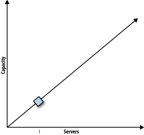
Figure 11-1. A system with one server
Now suppose that we add one more server, and the system’s capacity doubles, as shown in Figure 11-2.
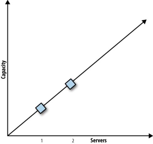
Figure 11-2. A linearly scalable system with two servers has twice the capacity
This is linear scalability. We doubled the number of servers, and as a result, we doubled the system’s capacity. Most systems aren’t linearly scalable; they often scale a bit like Figure 11-3 instead.
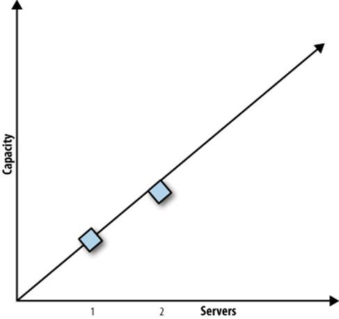
Figure 11-3. A system that doesn’t scale linearly
Most systems provide slightly less than linear scalability at small scaling factors, and the deviation from linearity becomes more obvious at higher scaling factors. In fact, most systems eventually reach a point of maximum throughput, beyond which additional investment provides a negativereturn—add more workload and you’ll actually reduce the system’s throughput![173]
How is this possible? Many models of scalability have been created over the years, with varying degrees of success and realism. The scalability model that we refer to here is based on some of the underlying mechanisms that influence systems as they scale. It is Dr. Neil J. Gunther’sUniversal Scalability Law (USL). Dr. Gunther has written about it at length in his books, including Guerrilla Capacity Planning (Springer). We will not go deeply into the mathematics here, but if you are interested, his book and the training courses offered by his company, Performance Dynamics, might be good resources for you.[174]
The short introduction to the USL is that the deviation from linear scalability can be modeled by two factors: a portion of the work cannot be done in parallel, and a portion of the work requires crosstalk. Modeling the first factor results in the well-known Amdahl’s Law, which causes throughput to level off. When part of the task can’t be parallelized, no matter how much you divide and conquer, the task takes at least as long as the serial portion.
Adding the second factor—intra-node or intra-process communication—to Amdahl’s Law results in the USL. The cost of this communication depends on the number of communication channels, which grows quadratically with respect to the number of workers in the system. Thus, the cost eventually grows faster than the benefit, and that’s what is responsible for retrograde scalability. Figure 11-4 illustrates the three concepts we’ve talked about so far: linear scaling, Amdahl scaling, and USL scaling. Most real systems look like the USL curve.
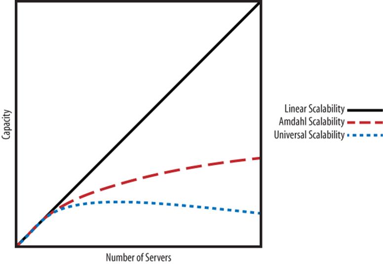
Figure 11-4. Comparison of linear scalability, Amdahl scalability, and the Universal Scalability Law
The USL can be applied both to hardware and to software. In the hardware case, the x-axis represents units of hardware, such as servers or CPUs; the workload, data size, and query complexity per unit of hardware must be held constant.[175] In the software case, the x-axis on the plot represents units of concurrency, such as users or threads; the workload per unit of concurrency must be held constant.
It is important to understand that the USL won’t describe any real system perfectly, because it is a simplified model. However, it is a good framework for understanding why systems fail to provide equal bang for the buck as they grow. It also reveals an important principle for building highly scalable systems: try to avoid serialization and crosstalk within the system.
It is possible to measure a system and use regression to determine the amount of seriality and crosstalk it exhibits. You can use this as a best-case upper bound for capacity planning and performance forecasting estimates. You can also examine how the system deviates from the USL model, using it as a worst-case lower bound to point out areas where your system isn’t performing as well as it should. In both cases, the USL gives you a reference to discuss scalability. Without it, you’d look at the system and not know what expectations you should have. A full exploration of this topic deserves its own book, and Dr. Gunther already wrote that, so we won’t go into this further.
Another framework for understanding scalability problems is the theory of constraints, which explains how to improve a system’s throughput and efficiency by reducing dependent events and statistical variations. It is explored in Eliyahu M. Goldratt’s book The Goal (North River), which is an extended parable about a manager at a manufacturing facility. Although it might seem far removed from the realm of a database server, the principles involved are the same as those in queueing theory and other aspects of operational research.
SCALABILITY MODELS AREN’T THE LAST WORD
This is all a lot of theory, but how well does it work in practice? Just as Newton’s laws turned out to be approximations that work reasonably well when you’re not close to the speed of light, these “scalability laws” are simplified models that work well in some cases. There’s a saying that all models are wrong, but some models are useful, and the USL in particular is useful for understanding some factors that contribute to poor scalability.
The USL breaks down when a workload’s interaction with the system on which it runs has subtleties. For example, one particularly common thing the USL fails to model well is the system’s changing behavior as a cluster’s total memory size changes relative to the dataset size. The USL doesn’t permit the possibility of better-than-linear scaling, but in the real world we sometimes see that happening as we add resources to a system and change a partially I/O-bound workload into a fully in-memory workload.
There are other cases where the USL model doesn’t describe a system’s behavior very well. It doesn’t model every possible way in which algorithmic complexity might change as systems change in size, or as the dataset changes. (The USL has an O(1) component and an O(N2) component, but what about the O(log N) component, or O(N log N), for example?) With some thought and practical experience, we could probably extend the USL to cover some of these common cases. However, that would turn a simple and usable model into a complex one that’s much harder to use. In practice, it’s quite good in a lot of cases, and it models enough of a system’s behavior that your brain can deal with the leftovers. That’s why we find it to be a nice compromise between correctness and usefulness.
In short: take the models with a grain of salt, and validate your findings when you use them.
[171] In the physical sciences, work per unit of time is called power, but in computing “power” is such an overloaded term that it’s ambiguous and we avoid it. However, a precise definition of capacity is the system’s maximum power output.
[172] Justin Bieber, we still love you!
[173] In fact, the term “return on investment” can also be considered in light of your financial investment. Upgrading a component to double its capacity often costs more than twice as much as the initial investment. Although we often consider this in the real world, we’ll omit it from our discussion here to avoid complicating an already confusing topic.
[174] You can also read our white paper, Forecasting MySQL Scalability with the Universal Scalability Law, which gives a condensed summary of the mathematics and principles at work in the USL. It is available at http://www.percona.com.
[175] In the real world, it is very difficult to define hardware scalability precisely, because it’s hard to actually hold all those variables constant as you vary the number of servers in the system.
Scaling MySQL
Placing all of your application’s data in a single MySQL instance simply will not scale well. Sooner or later you’ll hit performance bottlenecks. The traditional solution in many types of applications is to buy more powerful servers. This is what’s known as “scaling vertically” or “scaling up.” The opposite approach is to divide your work across many computers, which is usually called “scaling horizontally” or “scaling out.” We’ll discuss how to combine scale-out and scale-up solutions with consolidation, and how to scale with clustering solutions. Finally, most applications also have some data that’s rarely or never needed and that can be purged or archived. We call this approach “scaling back,” just to give it a name that matches the other strategies.
Planning for Scalability
People usually start to think about scalability when the server has difficulty keeping up with increased load. This usually shows up as a shift in workload from CPU-bound to I/O-bound, contention among concurrent queries, and increasing latency. Common culprits are increased query complexity, or a portion of the data or index that used to fit into memory but no longer does. You might see a change in certain types of queries and not others. For example, long or complex queries often show the strain before smaller queries.
If your application is highly scalable, you can simply plug in more servers to handle the load, and the performance problems will disappear. If it’s not scalable, you might find yourself fighting fires endlessly. You can avoid this by planning for scalability.
The hardest part of scalability planning is estimating how much load you’ll need to handle. You don’t need to get it exactly right, but you need to be within an order of magnitude. If you overestimate, you’ll waste resources on development, but if you underestimate, you’ll be unprepared for the load.
You also need to estimate your schedule approximately right—that is, you need to know where the “horizon” is. For some applications, a simple prototype could work fine for a few months, giving you a chance to raise capital and build a more scalable architecture. For other applications, you might need your current architecture to provide enough capacity for two years.
Here are some questions you can ask yourself to help plan for scalability:
§ How complete is your application’s functionality? A lot of the scaling solutions we suggest can make it harder to implement certain features. If you haven’t yet implemented some of your application’s core features, it might be hard to see how you can build them in a scaled application. Likewise, it could be hard to decide on a scaling solution before you’ve seen how these features will really work.
§ What is your expected peak load? Your application should work even at this load. What would happen if your site made the front page of Yahoo! News or Slashdot? Even if your application isn’t a popular website, you can still have peak loads. For example, if you’re an online retailer, the holiday season—especially the infamous online shopping days in the few weeks before Christmas—is often a time of peak load. In the US, Valentine’s Day and the weekend before Mother’s Day are also a peak times for online florists.
§ If you rely on every part of your system to handle the load, what will happen if part of it fails? For example, if you rely on replicas to distribute the read load, can you still keep up if one of them fails? Will you need to disable some functionality to do so? You can build in some spare capacity to help alleviate these concerns.
Buying Time Before Scaling
In a perfect world, you would be able to plan ahead for any eventuality, would always have enough developers, would never run into budget limitations, and so on. In the real world, things are usually more complicated, and you’ll need to make some compromises as you scale your application. In particular, you might need to put off big application changes for a while. Before we get deep into the details of scaling MySQL, here are some things you might be able to do now, before you make major scaling efforts:
Optimize performance
You can often get significant performance improvements from relatively simple changes, such as indexing tables correctly or switching from MyISAM to the InnoDB storage engine. If you’re facing performance limitations now, one of the first things you should do is enable and analyze the slow query log. See Chapter 3 for more on this topic.
There is a point of diminishing returns. After you’ve fixed most of the major problems, it gets harder and harder to improve performance. Each new optimization makes less of a difference and requires more effort, and they often make your application much more complicated.
Buy more powerful hardware
Upgrading your servers, or adding more of them, can sometimes work well. Especially for an application that’s early in its lifecycle, it’s often a good idea to buy a few more servers or get some more memory. The alternative might be to try to keep the application running on a single server. It can be more practical just to buy some more hardware than to change your application’s design, especially if time is critical and developers are scarce.
Buying more hardware works well if your application is either small or designed so it can use more hardware well. This is common for new applications, which are usually very small or reasonably well designed. For larger, older applications, buying more hardware might not work, or might be too expensive. For example, going from 1 to 3 servers isn’t a big deal, but going from 100 to 300 is a different story—it’s very expensive. At that point, it’s worth putting in a lot of time and effort to get as much performance as possible out of your existing systems.
Scaling Up
Scaling up means buying more powerful hardware, and for many applications this is all you need to do. There are many advantages to this strategy. A single server is so much easier to maintain and develop against than multiple servers that it offers significant cost savings, for example. Backing up and restoring your application on a single server is also simpler because there’s never any question about consistency or which dataset is the authoritative one. The reasons go on. Cost is complexity, and scaling up is simpler than scaling out.
You can scale up quite far. Commodity servers are readily available today with half a terabyte of memory, 32 or more CPU cores, and more I/O power than you can even use for MySQL (flash storage on PCIe cards, for example). With intelligent application and database design, and good performance optimization skills, you can build very large applications with MySQL on such servers.
How large can MySQL scale on modern hardware? Although it’s possible to run it on very powerful servers, it turns out that like most database servers, MySQL doesn’t scale perfectly (surprise!) as you add hardware resources. To run MySQL on big-iron boxes, you will definitely need a recent version of the server. The MySQL 5.0 and 5.1 series will choke badly on such large hardware, due to internal scalability issues. You will need either MySQL 5.5 or newer, or Percona Server 5.1 or newer. Even so, the currently reasonable “point of diminishing returns” is probably somewhere around 256 GB of RAM, 32 cores, and a PCIe flash drive. MySQL will continue to provide improved performance on bigger hardware than that, but the price-to-performance ratio will not be as good, and in fact even on these systems you can often get much better performance by running several smaller instances of MySQL instead of one big instance that uses all of the server’s resources. This is a rapidly moving target, so this advice will probably be out of date pretty soon.
Scaling up can work for a while, and many applications will not outgrow this strategy, but if your application grows extremely large[176] it ultimately won’t work. The first reason is money. Regardless of what software you’re running on the server, at some point scaling up will become a bad financial decision. Outside the range of hardware that offers the best price-to-performance ratio, the hardware tends to become more proprietary and unusual, and correspondingly more expensive. This means there’s a practical limit on how far up you can afford to scale. If you use replication and upgrade your master to high-end hardware, there’s also little chance that you’ll be able to build a replica server that’s powerful enough to keep up. A heavily loaded master can easily do more work than a replica server with the same hardware can handle, because the replication thread can’t use multiple CPUs and disks efficiently.
Finally, you can’t scale up indefinitely, because even the most powerful computers have limits. Single-server applications usually run into read limits first, especially if they run complicated read queries. Such queries are single-threaded inside MySQL, so they’ll use only one CPU, and money can’t buy them much more performance. The fastest server-grade CPUs you can buy are only a couple of times faster than commodity CPUs. Adding many CPUs or CPU cores won’t help the slow queries run faster. The server will also begin to run into memory limits as your data becomes too large to cache effectively. This will usually show up as heavy disk usage, and disks are the slowest parts of modern computers.
The most obvious place where you can’t scale up is in the cloud. You generally can’t get very powerful servers in most public clouds, so scaling up is not an option if your application must grow very large. We’ll discuss this topic further in Chapter 13.
As a result, we recommend that you don’t plan to scale up indefinitely if the prospect of a hitting a scalability ceiling is real and would be a serious business problem. If you know your application will grow very large, it’s fine to buy a more powerful server for the short term while you work on another solution. However, in general you’ll ultimately have to scale out, which brings us to our next topic.
Scaling Out
We can lump scale-out tactics into three broad groups: replication, partitioning, and sharding.
The simplest and most common way to scale out is to distribute your data across several servers with replication, and then use the replicas for read queries. This technique can work well for a read-heavy application. It has drawbacks, such as cache duplication, but even that might not be a severe problem if the data size is limited. We wrote quite a bit about these issues in the previous chapter, and we’ll return to them later in this one.
The other common way to scale out is to partition your workload across multiple “nodes.” Exactly how you partition the workload is an intricate decision. Most large MySQL applications don’t automate the partitioning, at least not completely. In this section, we take a look at some of the possibilities for partitioning and explore their strengths and drawbacks.
A node is the functional unit in your MySQL architecture. If you’re not planning for redundancy and high availability, a node might be one server. If you’re designing a redundant system with failover, a node is generally one of the following:
§ A master-master replication pair, with an active server and a passive replica
§ A master and many replicas
§ An active server that uses a distributed replicated block device (DRBD) for a standby
§ A SAN-based “cluster”
In most cases, all servers within a node should have the same data. We like the master-master replication architecture for two-server active-passive nodes.
Functional partitioning
Functional partitioning, or division of duties, means dedicating different nodes to different tasks. We’ve mentioned some similar approaches before; for example, we wrote about how to design different servers for OLTP and OLAP workloads in the previous chapter. Functional partitioning usually takes that strategy even further by dedicating individual servers or nodes to different applications, so each contains only the data its particular application needs.
We’re using the word “application” a bit broadly here. We don’t mean a single computer program, but a set of related programs that’s easily separated from other, unrelated programs. For example, if you have a website with distinct sections that don’t need to share data, you can partition by functional area on the website. It’s common to see portals that tie the different areas together; from the portal, you can browse to the news section of the site, the forums, the support area and knowledge base, and so on. The data for each of these functional areas could be on a dedicated MySQL server. Figure 11-5 depicts this arrangement.
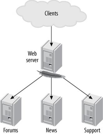
Figure 11-5. A portal and nodes dedicated to functional areas
If the application is huge, each functional area can also have its own dedicated web server, but that’s less common.
Another possible functional partitioning approach is to split a single application’s data by determining sets of tables that you never join to each other. If it becomes necessary, you can usually perform a few such joins in the application if they’re not performance-critical. There are a few variations on this approach, but they have the common property that each type of data can be found on only a single node. This is not a common way to partition data, because it’s very difficult to do effectively and it doesn’t offer any advantages over other methods.
In the final analysis, you still can’t scale functional partitioning indefinitely, because each functional area must scale vertically if it is tied to a single MySQL node. One of the applications or functional areas is likely to eventually grow too large, forcing you to find a different strategy. And if you take functional partitioning too far, it can be harder to change to a more scalable design later.
Data sharding
Data sharding[177] is the most common and successful approach for scaling today’s very large MySQL applications. You shard the data by splitting it into smaller pieces, or shards, and storing them on different nodes.
Sharding works well when combined with some type of functional partitioning. Most sharded systems also have some “global” data that isn’t sharded at all (say, lists of cities, or login data). This global data is usually stored on a single node, often behind a cache such as memcached.
In fact, most applications shard only the data that needs sharding—typically, the parts of the dataset that will grow very large. Suppose you’re building a blogging service. If you expect 10 million users, you might not need to shard the user registration information because you might be able to fit all of the users (or the active subset of them) entirely in memory. If you expect 500 million users, on the other hand, you should probably shard this data. The user-generated content, such as posts and comments, will almost certainly require sharding in either case, because these records are much larger and there are many more of them.
Large applications might have several logical datasets that you can shard differently. You can store them on different sets of servers, but you don’t have to. You can also shard the same data multiple ways, depending on how you access it. We show an example of this approach later.
Sharding is dramatically different from the way most applications are designed initially, and it can be difficult to change an application from a monolithic data store to a sharded architecture. That’s why it’s much easier to build an application with a sharded data store from the start if you anticipate that it will eventually need one.
Most applications that don’t build in sharding from the beginning go through stages as they get larger. For example, you can use replication to scale read queries on your blogging service until it doesn’t work any more. Then you can split the service into three parts: users, posts, and comments. You can place these on different servers (functional partitioning), perhaps with a service-oriented architecture, and perform the joins in the application. Figure 11-6 shows the evolution from a single server to functional partitioning.
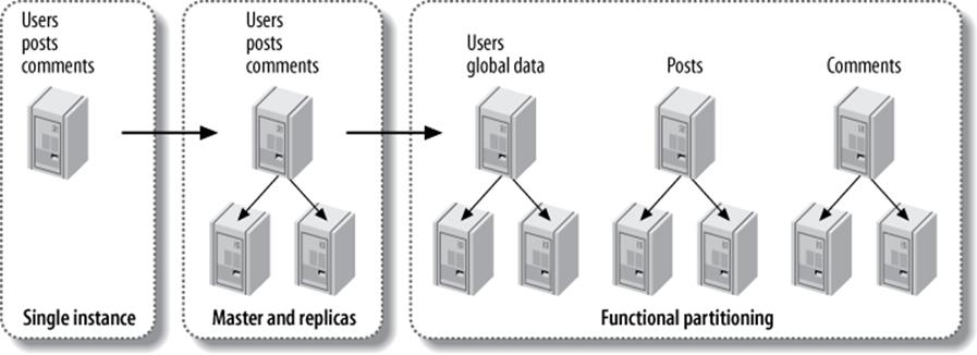
Figure 11-6. From a single instance to a functionally partitioned data store
Finally, you can shard the posts and comments by the user ID, and keep the user information on a single node. If you keep a master-replica configuration for the global node and use master-master pairs for the sharded nodes, the final data store might look like Figure 11-7.
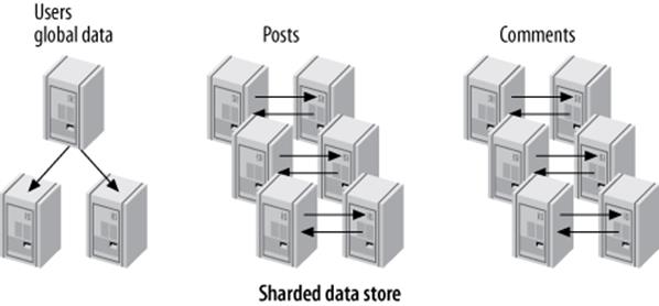
Figure 11-7. A data store with one global node and six master-master nodes
If you know in advance that you’ll need to scale very large, and you know the limitations of functional partitioning, you might choose to skip the steps in the middle and go straight from a single node to a sharded data store. In fact, foresight can often help you avoid ugly sharding schemes that might arise from meeting each challenge as it comes.
Sharded applications often have a database abstraction library that eases the communication between the application and the sharded data store. Such libraries usually don’t hide the sharding completely, because the application usually knows something about a query that the data store doesn’t. Too much abstraction can cause inefficiencies, such as querying all nodes for data that lives on a single node.
A sharded data store might feel like an elegant solution, but it’s hard to build. So why choose this architecture? The answer is simple: if you want to scale your write capacity, you must partition your data. You cannot scale write capacity if you have only a single master, no matter how many replicas you have. Sharding, for all its drawbacks, is our preferred solution to this problem.
TO SHARD OR NOT TO SHARD?
That is the question, isn’t it? Here’s the simple answer: don’t shard unless you need to. See if you can delay it via performance optimization or a better application or database design. If you can put off sharding long enough, you might be able to just buy a bigger server, upgrade MySQL to a new higher-performance version, and keep on chugging with a single server, plus or minus replication.
In a nutshell, sharding is inevitable when either the data size or the write workload becomes too much for a single server. You’d be surprised how far systems can be scaled without sharding, using intelligent application design. Some very popular applications you’d probably assume were sharded from day one in fact grew to multi-billion-dollar valuations and insane amounts of traffic without sharding. It’s not the only game in town, and it’s a tough way to build an application if it’s not needed.
Choosing a partitioning key
The most important challenge with sharding is finding and retrieving data. How you find data depends on how you shard it. There are many ways to do this, and some are better than others.
The goal is to make your most important and frequent queries touch as few shards as possible (remember, one of the scalability principles is to avoid crosstalk between nodes). The most important part of that process is choosing a partitioning key (or keys) for your data. The partitioning key determines which rows should go onto each shard. If you know an object’s partitioning key, you can answer two questions:
§ Where should I store this data?
§ Where can I find the data I need to fetch?
We’ll show you a variety of ways to choose and use a partitioning key later. For now, let’s look at an example. Suppose we do as MySQL’s NDB Cluster does, and use a hash of each table’s primary key to partition the data across all the shards. This is a very simple approach, but it doesn’t scale well because it frequently requires you to check all the shards for the data you want. For example, if you want user 3’s blog posts, where can you find them? They are probably scattered evenly across all the shards, because they’re partitioned by the primary key, not by the user. Using a primary key hash makes it simple to know where to store the data, but it might make it harder to fetch it, depending on which data you need and whether you know the primary key.
Cross-shard queries are worse than single-shard queries, but as long as you don’t touch too many shards, they might not be too bad. The worst case is when you have no idea where the desired data is stored, and you need to scan every shard to find it.
A good partitioning key is usually the primary key of a very important entity in the database. These keys determine the unit of sharding. For example, if you partition your data by a user ID or a client ID, the unit of sharding is the user or client.
A good way to start is to diagram your data model with an entity-relationship diagram, or an equivalent tool that shows all the entities and their relationships. Try to lay out the diagram so that the related entities are close together. You can often inspect such a diagram visually and find candidates for partitioning keys that you’d otherwise miss. Don’t just look at the diagram, though; consider your application’s queries as well. Even if two entities are related in some way, if you seldom or never join on the relationship, you can break the relationship to implement the sharding.
Some data models are easier to shard than others, depending on the degree of connectivity in the entity-relationship graph. Figure 11-8 depicts an easily sharded data model on the left, and one that’s difficult to shard on the right.
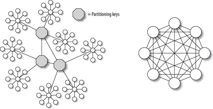
Figure 11-8. Two data models, one easy to shard and the other difficult [178]
The data model on the left is easy to shard because it has many connected subgraphs consisting mostly of nodes with just one connection, and you can “cut” the connections between the subgraphs relatively easily. The model on the right is hard to shard, because there are no such subgraphs. Most data models, luckily, look more like the lefthand diagram than the righthand one.
When choosing a partitioning key, try to pick something that lets you avoid cross-shard queries as much as possible, but also makes shards small enough that you won’t have problems with disproportionately large chunks of data. You want the shards to end up uniformly small, if possible, and if not, at least small enough that they’re easy to balance by grouping different numbers of shards together. For example, if your application is US-only and you want to divide your dataset into 20 shards, you probably shouldn’t shard by state, because California has such a huge population. But you could shard by county or telephone area code, because even though these won’t be uniformly populated, there are enough of them that you can still choose 20 sets that will be roughly equally populated in total, and you can choose them with an affinity that helps avoid cross-shard queries.
Multiple partitioning keys
Complicated data models make data sharding more difficult. Many applications have more than one partitioning key, especially if there are two or more important “dimensions” in the data. In other words, the application might need to see an efficient, coherent view of the data from different angles. This means you might need to store at least some data twice within the system.
For example, you might need to shard your blogging application’s data by both the user ID and the post ID, because these are two common ways the application looks at the data. Think of it this way: you frequently want to see all posts for a user, and all comments for a post. But sharding by user doesn’t help you find comments for a post, and sharding by post doesn’t help you find posts for a user. If you need both types of queries to touch only a single shard, you’ll have to shard both ways.
Just because you need multiple partitioning keys doesn’t mean you’ll need to design two completely redundant data stores. Let’s look at another example: a social networking book club website, where the site’s users can comment on books. The website can display all comments for a all book, as well as all books a user has read and commented on.
You might build one sharded data store for the user data and another for the book data. Comments have both a user ID and a post ID, so they cross the boundaries between shards. Instead of completely duplicating comments, you can store the comments with the user data. Then you can store just a comment’s headline and ID with the book data. This might be enough to render most views of a book’s comments without accessing both data stores, and if you need to display the complete comment text, you can retrieve it from the user data store.
Querying across shards
Most sharded applications have at least some queries that need to aggregate or join data from multiple shards. For example, if the book club site shows the most popular or active users, it must by definition access every shard. Making such queries work well is the most difficult part of implementing data sharding, because what the application sees as a single query needs to be split up and executed in parallel as many queries, one per shard. A good database abstraction layer can help ease the pain, but even then such queries are so much slower and more expensive than in-shard queries that aggressive caching is usually necessary as well.
Some languages, such as PHP, don’t have good support for executing multiple queries in parallel. A common way to work around this is to build a helper application, often in C or Java, to execute the queries and aggregate the results. The PHP application then queries the helper application, which is often a web service or a worker service such as Gearman.
Cross-shard queries can also benefit from summary tables. You can build them by traversing all the shards and storing the results redundantly on each shard when they’re complete. If duplicating the data on each shard would be too wasteful, you can consolidate the summary tables onto another data store, so they’re stored only once.
Nonsharded data often lives in the global node, with heavy caching to shield it from the load.
Some applications use essentially random sharding when perfectly even data distribution is important, or when there is no good partitioning key. A distributed search application is a good example. In this case, cross-shard queries and aggregation are the norm, not the exception.
Querying across shards isn’t the only thing that’s harder with sharding. Maintaining data consistency is also difficult. Foreign keys won’t work across shards, so the normal solution is to check referential integrity as needed in the application, or use foreign keys within a shard, because internal consistency within a shard might be the most important thing. It’s possible to use XA transactions, but this is uncommon in practice because of the overhead.
You can also design cleanup processes that run intermittently. For example, if a user’s book club account expires, you don’t have to remove it immediately. You can write a periodic job to remove the user’s comments from the per-book shard, and you can build a checker script that runs periodically and makes sure the data is consistent across the shards.
Allocating data, shards, and nodes
Shards and nodes don’t have to have a one-to-one relationship. It’s often a good idea to make a shard’s size much smaller than a node’s capacity, so you can store multiple shards on a single node.
Keeping each shard small helps keep the data manageable. It makes it easier to do database backups and recovery, and if the tables are small, it can ease jobs such as schema changes. For example, suppose you have a 100 GB table that you can either store as it is or split into 100 shards of 1 GB tables, which you would store on a single node. Now suppose you want to add an index to the table(s). This would take much longer on a 100 GB shard than it would on all the 1 GB shards combined, because the 1 GB shards fit completely in memory. You also might need to make the data unavailable while ALTER TABLE is running, and blocking 1 GB of data is much better than blocking 100 GB.
Smaller shards are easier to move around, too. This makes it easier to reallocate capacity and rebalance the shards among the nodes. Moving a shard is generally not an efficient process. You typically need to put the affected shard into read-only mode (a feature you’ll need to build into your application), extract the data, and move it to another node. This usually involves using mysqldump to export the data and mysql to reload it. If you’re using Percona Server, you can use XtraBackup to move the files between servers, which is much more efficient than dumping and reloading.
In addition to moving shards between nodes, you might need to think about moving data between shards, preferably without interrupting service for the whole application. If your shards are large, it will be harder to balance capacity by moving entire shards around, so you’ll probably need a way to move the individual bits of data (for example, a single user) between shards. Moving data between shards is usually a lot more complicated than just moving shards, so it’s best not to do it if possible. That’s one reason we recommend keeping the shard size manageable.
The relative size of your shards depends on the application’s needs. As a rough guide, a “manageable size” for us is one that keeps tables small enough that we can perform regular maintenance jobs, such as ALTER TABLE, CHECK TABLE, or OPTIMIZE TABLE, within 5 or 10 minutes.
If you make your shards too small, you might end up with too many tables, which can cause problems with the filesystem or MySQL’s internal structures. Small shards might also increase the number of cross-shard queries you need to make.
Arranging shards on nodes
You’ll need to decide how you want to arrange the shards on a node. Here are some common methods:
§ Use a single database per shard, and use the same name for each shard’s database. This method is typical when you want each shard to mirror the original application’s structure. It can work well when you’re making many application instances, each of which is aware of only one shard.
§ Place tables from several shards into one database, and include the shard number in each table’s name (e.g., bookclub.comments_23). A single database can hold multiple shards in this configuration.
§ Use a single database per shard, and include all the application’s tables in the database. Include the shard number in the database name but not the table name (e.g., the tables might be named bookclub_23.comments, bookclub_23.users, and so on). This is common when an application connects to a single database and doesn’t specify the database name in any of its queries. The advantage is that you don’t need to customize the queries per shard, and it can ease the transition to sharding for an application that uses only one database.
§ Use a single database per shard, and include the shard number in both the database and table names (e.g., the table name would become bookclub_23.comments_23).
§ Run multiple MySQL instances per node, each with one or more shards, arranged in any sensible combination of the ways we’ve just mentioned.
If you include the shard number in the table name, you’ll need some way to insert the shard number into templated queries. Typical practices include special “magic” placeholder values in queries, sprintf()-style formatting specifications such as %s, and string interpolation with variables. Here is one way you can create templated queries in PHP:
$sql = "SELECT book_id, book_title FROM bookclub_%d.comments_%d... ";
$res = mysql_query(sprintf($sql, $shardno, $shardno), $conn);
You could also just use string interpolation:
$sql = "SELECT book_id, book_title FROM bookclub_$shardno.comments_$shardno ...";
$res = mysql_query($sql, $conn);
This is easy to build into a new application, but it might be harder for existing applications. When we’re building new applications and query templating isn’t an issue, we like to use a single database per shard, with the shard number in both the database and the table name. It adds some complexity for jobs such as scripting ALTER TABLE, but it has advantages, too:
§ You can move a shard easily if it’s completely contained in a single database.
§ Because a database is a directory in the filesystem, you can manage a shard’s files easily.
§ It’s easy to find out how large the shard is if it isn’t mixed up with other shards.
§ The globally unique table names help avoid mistakes. If table names are the same everywhere, it’s easy to accidentally query the wrong shard because you connected to the wrong node, or import one shard’s data into another shard’s tables.
You might want to consider whether your application’s data has any shard affinity. You might benefit from placing certain shards “near” each other (on the same server, on the same subnet, in the same data center, or on the same switch) to exploit some similarity in the data access patterns. For example, you can shard by user and then place users from the same country into shards on the same nodes.
Adding sharding support to an existing application often results in one shard per node. This simplification helps limit how much you need to change the application’s queries. Sharding is usually a pretty disruptive change for an application, so it makes sense to simplify where possible. If you shard so each node looks like a miniature copy of the whole application’s data, you might not have to change most of the queries or worry about routing queries to the desired node.
Fixed allocation
There are two main ways to allocate data to shards: the fixed and dynamic allocation strategies. Both require a partitioning function that takes a row’s partitioning key as input and returns the shard that holds the row.[179]
Fixed allocation uses a partitioning function that depends only on the partitioning key’s value. Hash functions and modulus are good examples. These functions map each value of the partitioning key into a limited number of “buckets” that can hold the data.
Suppose you want 100 buckets, and you want to find out where to put user 111. If you’re using a modulus, the answer is easy: 111 modulus 100 is 11, so you should place the user into shard 11.
If, on the other hand, you’re using the CRC32() function for hashing, the answer is 81:
mysql> SELECT CRC32(111) % 100;
+------------------+
| CRC32(111) % 100 |
+------------------+
| 81 |
+------------------+
The primary advantages of a fixed strategy are simplicity and low overhead. You can also hardcode it into the application.
However, a fixed allocation strategy has disadvantages, too:
§ If the shards are large and there are few of them, it can be hard to balance the load across shards.
§ Fixed allocation doesn’t let you decide where to store each piece of data, which is important for applications that don’t have a very uniform load on the unit of sharding. Some pieces of data will likely be much more active than others, and if many of those happen to fall into the same shard, a fixed allocation strategy doesn’t let you ease the strain by moving some of them to another shard. (This is not as much of a problem when you have many small pieces of data in each shard, because the law of large numbers will help even things out.)
§ It’s usually harder to change the sharding, because it requires reallocating existing data. For example, if you’ve sharded by a hash function modulus 10, you’ll have 10 shards. If the application grows and the shards get too large, you might want to increase the number of shards to 20. That will require rehashing everything, updating a lot of data, and moving data between shards.
Because of these limitations, we usually prefer dynamic allocation for new applications. But if you’re sharding an existing application, you might find it easier to build a fixed allocation strategy instead of a dynamic one, because it’s simpler. That said, most applications that use fixed allocation end up with a dynamic allocation strategy sooner or later.
Dynamic allocation
The alternative to fixed allocation is a dynamic allocation strategy that you store separately, mapping each unit of data to a shard. An example is a two-column table of user IDs and shard IDs:
CREATE TABLE user_to_shard (
user_id INT NOT NULL,
shard_id INT NOT NULL,
PRIMARY KEY (user_id)
);
The table itself is the partitioning function. Given a value for the partitioning key (the user ID), you can find the shard ID. If the row doesn’t exist, you can pick the desired shard and add it to the table. You can also change it later—that’s what makes this a dynamic allocation strategy.
Dynamic allocation adds overhead to the partitioning function because it requires a call to an external resource, such as a directory server (a data storage node that stores the mapping). Such an architecture often needs more layers for efficiency. For example, you can use a distributed caching system to store the directory server’s data in memory, because in practice it doesn’t change all that much. Or—perhaps more commonly—you can just add a shard_id column to the users table and store it there.
The biggest advantage of dynamic allocation is fine-grained control over where the data is stored. This makes it easier to allocate data to the shards evenly and gives you a lot of flexibility to accommodate changes you don’t foresee.
A dynamic mapping also lets you build multiple levels of sharding strategies on top of the simple key-to-shard mapping. For example, you can build a dual mapping that assigns each unit of sharding to a group (e.g., a group of users in the book club), and then keeps the groups together on a shard where possible. This lets you take advantage of shard affinities, so you can avoid cross-shard queries.
If you use a dynamic allocation strategy, you can have imbalanced shards. This can be useful when your servers aren’t all equally powerful, or when you want to use some of them for different purposes, such as archived data. If you also have the ability to rebalance shards at any time, you can maintain a one-to-one mapping of shards to nodes without wasting capacity. Some people prefer the simplicity of one shard per node. (But remember, there are advantages to keeping shards small.)
Dynamic allocation and smart use of shard affinities can prevent your cross-shard queries from growing as you scale. Imagine a cross-shard query in a data store with four nodes. In a fixed allocation, any given query might require touching all shards, but a dynamic allocation strategy might let you run the same query on only three of the nodes. This might not seem like a big difference, but consider what will happen when your data store grows to 400 shards: the fixed allocation will require querying all 400 shards, while the dynamic allocation might still require querying only 3.
Dynamic allocation lets you make your sharding strategy as complex as you wish. Fixed allocation doesn’t give you as many choices.
Mixing dynamic and fixed allocation
You can use a mixture of fixed and dynamic allocation, which is often helpful and sometimes required. Dynamic allocation works well when the directory mapping isn’t too large. If there are many units of sharding, it might not work so well.
An example is a system that’s designed to store links between websites. Such a site needs to store tens of billions of rows, and the partitioning key is the combination of source and target URLs. (Just one of the two URLs might have hundreds of millions of links, so neither URL is selective enough by itself.) However, it’s not feasible to store all of the source and target URL combinations in the mapping table, because there are many of them, and each URL requires a lot of storage space.
One solution is to concatenate the URLs and hash them into a fixed number of buckets, which you can then map dynamically to shards. If you make the number of buckets large enough—say, a million—you’ll be able to fit quite a few of them into each shard. The result is that you get most of the benefits of dynamic sharding, without having a huge mapping table.
Explicit allocation
A third allocation strategy is to let the application choose each row’s desired shard explicitly when it creates the row. This is harder to do with existing data, so it’s not very common when adding sharding to an application. However, it can be helpful sometimes.
The idea is to encode the shard number into the ID, similar to the technique we showed for avoiding duplicate key values in master-master replication. (See Writing to Both Masters in Master-Master Replication for more details.)
For example, suppose your application wants to create user 3 and assign it to shard 11, and you’ve reserved the eight most significant bits of a BIGINT column for the shard number. The resulting ID value is (11 << 56) + 3, or 792633534417207299. The application can easily extract the user ID and the shard ID later. Here’s an example:
mysql> SELECT (792633534417207299 >> 56) AS shard_id,
-> 792633534417207299 & ~(11 << 56) AS user_id;
+----------+---------+
| shard_id | user_id |
+----------+---------+
| 11 | 3 |
+----------+---------+
Now suppose you want to create a comment for this user and store it in the same shard. The application can assign the comment ID 5 for the user, and combine the value 5 with the shard ID 11 in the same way.
The benefit of this approach is that each object’s ID carries its partitioning key along with it, whereas other approaches usually require a join or another lookup to find the partitioning key. If you want to retrieve a certain comment from the database, you don’t need to know which user owns it; the object’s ID tells you where to find it. If the object were sharded dynamically by user ID, you’d have to find the comment’s user, then ask the directory server which shard to look on.
Another solution is to store the partitioning key together with the object in separate columns. For example, you’d never refer just to comment 5, but to comment 5 belonging to user 3. This approach will probably make some people happier, because it doesn’t violate first normal form; however, the extra column causes more overhead, coding, and inconvenience. (This is one case where we feel there’s an advantage to storing two values in a single column.)
The drawback of explicit allocation is that the sharding is fixed, and it’s harder to balance shards. On the other hand, this approach works well with the combination of fixed and dynamic allocation. Instead of hashing to a fixed number of buckets and mapping these to nodes, you encode the bucket as part of each object. This gives the application control over where the data is located, so it can place related data together on the same shard.
BoardReader (http://boardreader.com) uses a variation of this technique: it encodes the partitioning key in the Sphinx document ID. This makes it easy to find each search result’s related data in the sharded data store. See Appendix F for more on Sphinx.
We’ve described mixed allocation because we’ve seen cases where it’s useful, but normally we don’t recommend it. We like to use dynamic allocation when possible, and avoid explicit allocation.
Rebalancing shards
If necessary, you can move data to different shards to rebalance the load. For example, many readers have probably heard developers from large photo-sharing sites or popular social networking sites mention their tools for moving users to different shards.
The ability to move data between shards has its benefits. For example, it can help you upgrade your hardware by enabling you to move users off the old shard onto the new one without taking the whole shard down or making it read-only.
However, we like to avoid rebalancing shards if possible, because it can disrupt service to your users. Moving data between shards also makes it harder to add features to the application, because new features might have to include an upgrade to the rebalance script. If you keep your shards small enough, you might not need to do this; you can often rebalance the load by moving entire shards, which is easier than moving part of a shard (and more efficient, in terms of cost per row of data).
One strategy that works well is to use a dynamic sharding strategy and assign new data to shards randomly. When a shard gets full enough, you can set a flag that tells the application not to give it any new data. You can then flip the flag back if you want more data on that shard in the future.
Suppose you install a new MySQL node and place 100 shards on it. To begin, you set their flags to 1, so the application knows they’re ready for new data. Once they each have enough data (10,000 users each, for example), you set their flags to 0. Then, if the node becomes underloaded after a while because of abandoned accounts, you can reopen some of the shards and add new users to them.
If you upgrade the application and add features that make each shard’s query load higher, or if you just miscalculated the load, you can move some of the shards to new nodes to ease the load. The drawback is that an entire shard might be read-only or offline while you do this. It’s up to you and your users to decide whether that’s acceptable.
Another tactic we use a lot is to set up two replicas of a shard, each with a complete copy of the shard’s data. We then make each replica responsible for half of the data, and stop sending queries to the master completely. Each replica contains some data it doesn’t use; we set up a background job with a tool such as Percona Toolkit’s pt-archiver to remove the unwanted data. This is simple and requires practically zero downtime.
Generating globally unique IDs
When you convert a system to use a sharded data store, you frequently need to generate globally unique IDs on many machines. A monolithic data store often uses AUTO_INCREMENT columns for this purpose, but that doesn’t tend to work well across many servers. There are several ways to solve this problem:
Use auto_increment_increment and auto_increment_offset
These two server settings instruct MySQL to increment AUTO_INCREMENT columns by a desired value and to begin numbering from a desired offset. For example, in the simplest case with two servers, you can configure the servers to increment by two, set one server’s offset to one, and set the other’s to two (you can’t set either value to zero). Now one server’s columns will always contain even numbers, and the other’s will always contain odd numbers. The setting applies to all tables in the server.
Because of its simplicity and lack of dependency on a central node, this is a popular way to generate values, but it requires you to be careful with your server configurations. It’s easy to accidentally configure servers so that they generate duplicate numbers, especially if you move them into different roles as you add more servers, or when you recover from failures.
Create a table in the global node
You can create a table with an AUTO_INCREMENT column in your global database node, and applications can use this to generate unique numbers.
Use memcached
There’s an incr() function in the memcached API that can increment a number atomically and return the result. You can use Redis, too.
Allocate numbers in batches
The application can request a batch of numbers from a global node, use all the numbers, and then request more.
Use a combination of values
You can use a combination of values, such as the shard ID and an incrementing number, to make each server’s values unique. See the discussion of this technique in the previous section.
Use GUID values
You can generate globally unique values with the UUID() function. Beware, though: this function does not replicate correctly with statement-based replication, although it works fine if your application selects the value into its own memory and then uses it as a literal in statements. GUID values are large and nonsequential, so they don’t make good primary keys for InnoDB tables. See Inserting rows in primary key order with InnoDB for more on this. There’s also a UUID_SHORT() function in MySQL 5.1 and newer versions, which has some nice properties such as being sequential and only 64 bits instead of 128.
If you use a global allocator to generate values, be careful that the single point of contention doesn’t create a bottleneck for your application.
Although the memcached approach can be very fast (tens of thousands of values per second), it isn’t persistent. Each time you restart the memcached service, you’ll need to initialize the value in the cache. This could require you to find the maximum value that’s in use across all shards, which might be very slow and difficult to do atomically.
Tools for sharding
One of the first things you’ll have to do when designing a sharded application is write code for querying multiple data sources.
It’s generally a poor design to expose the multiple data sources to the application without any abstraction, because it can add a lot of code complexity. It’s better to hide the data sources behind an abstraction layer. This layer might handle the following tasks:
§ Connecting to the correct shard and querying it
§ Distributed consistency checks
§ Aggregating results across shards
§ Cross-shard joins
§ Locking and transaction management
§ Creating shards (or at least discovering new shards on the fly) and rebalancing shards if you have time to implement this
You might not have to build your own sharding infrastructure from scratch. There are several tools and systems that either provide some of the necessary functionality or are specifically designed to implement a sharded architecture.
One database abstraction layer with sharding support is Hibernate Shards (http://shards.hibernate.org), Google’s extension to the open source Java-based Hibernate object-relational mapping (ORM) library. It provides shard-aware implementations of the Hibernate Core interfaces, so applications don’t necessarily have to be redesigned to use a sharded data store; in fact, they might not even have to be aware that they’re using one. Hibernate Shards uses a fixed allocation strategy to allocate data to the shards. Another Java sharding system is HiveDB (http://www.hivedb.org).
In PHP, you can use Justin Swanhart’s Shard-Query system (http://code.google.com/p/shard-query/), which automatically decomposes queries, executes them in parallel, and combines the results. Commercial systems targeted at similar use cases are ScaleBase (http://www.scalebase.com),ScalArc (http://www.scalarc.com), and dbShards (http://www.dbshards.com).
Sphinx is a full-text search engine, not a sharded data storage and retrieval system, but it is still useful for some types of queries across sharded data stores. It can query remote systems in parallel and aggregate the results. Sphinx is discussed further in Appendix F.
Scaling by Consolidation
A heavily sharded architecture creates an opportunity to get more out of your hardware. Our research and experience have shown that MySQL can’t use the full power of modern hardware. As you scale beyond about 24 CPU cores, MySQL’s efficiency starts to level off. A similar thing happens beyond 128 MB of memory, and MySQL can’t even come close to using the full I/O power of high-end PCIe flash devices such as Virident and Fusion-io cards.
Instead of using a single server instance on a powerful machine, there’s another option. You can make your shards small enough that you can fit several per machine (a practice we’ve been advocating anyway), and run several instances per server, carving up the server’s physical resources to give each instance a portion.
This actually works, although we wish it weren’t necessary. It’s a combination of the scale-up and scale-out approaches. You can do it in other ways—you don’t have to use sharding—but sharding is a natural fit for consolidation on large servers.
Some people like to achieve consolidation with virtualization, which has its benefits. But virtualization also has a pretty hefty performance cost itself in many cases. It depends on the technology, but it’s usually noticeable, and the overhead is especially exaggerated when I/O is very fast. As an alternative, you can run multiple MySQL instances, each listening on different network ports or binding to different IP addresses.
We’ve been able to achieve a consolidation factor of up to 10x or 15x on powerful hardware. You’ll have to balance the cost of the administrative complexity with the benefit of better performance to determine what’s best for you.
At this point, the network is likely to become the bottleneck—a problem most MySQL users don’t run into very often. You can address the problem by using multiple NICs and bonding them. The Linux kernel isn’t ideal for this, depending on the version, because older kernels can use only one CPU for network interrupts per bonded device. As a result, you shouldn’t bond too many cables into too few virtual devices, or you’ll run into a different network bottleneck inside the kernel. Newer kernels should help with this, so check your distribution to find out what your options are.
Another way you can get more out of this strategy is to bind each MySQL instance to specific cores. This helps for two reasons: first because MySQL gets more performance per core at lower core counts due to its internal scalability limitations, and second when an instance is running threads on many cores, there’s less overhead due to synchronizing shared data between the cores. This helps avoid the scalability limitations of the hardware itself. Limiting MySQL to only some cores can reduce the crosstalk between CPU cores. Notice the recurring theme? Pin the process to cores that are on the same physical socket for the best results.
Scaling by Clustering
The dream scenario for scaling is a single logical database that can hold as much data, serve as many queries, and grow as large as you need it to. Many people’s first thought is to create a “cluster” or “grid” that handles this seamlessly, so the application doesn’t need to do any dirty work or know that the data really lives in many servers instead of just one. With the rise of the cloud, autoscaling—dynamically adding servers to or removing them from the cluster in response to changes in workload or data size—is also becoming interesting.
In the second edition of this book, we expressed our regret that the available technology wasn’t really up to the task. Since then, a lot of the buzz has centered around so-called NoSQL technologies. Many NoSQL proponents made strange and unsubstantiated claims such as “the relational model can’t scale,” or “SQL can’t scale.” New concepts emerged, and new catchphrases were on everyone’s lips. Who hasn’t heard of eventual consistency, BASE, vector clocks, or the CAP theorem these days?
But as time has passed, sanity has been at least partially restored. Experience is beginning to reveal that many of the NoSQL databases are primitive in their own ways and aren’t really up to a lot of tasks themselves.[180] In the meantime, a variety of SQL-based technologies have arisen—whatMatt Aslett of the 451 Group calls NewSQL databases. What’s the difference between SQL and NewSQL? The NewSQL databases are setting out to prove that SQL and relational technology aren’t the problem. Rather, the scalability problems in relational databases are implementation problems, and new implementations are showing better results.
Is everything old new again? Yes and no. A lot of the high-performance implementations of clustered relational databases are built on low-level building blocks that look remarkably like NoSQL databases, especially key-value stores. For example, NDB Cluster isn’t a SQL database; it’s a scalable database that can be accessed through its native API, which is very much NoSQL, but it can also talk SQL when you put a MySQL storage engine in front of it. It is a fully distributed, shared-nothing, high-performance, auto-sharded, transactional database server with no single point of failure. It’s a very advanced database that has no equal for particular uses. And it has become much more powerful, sophisticated, and general-purpose in the last few years. At the same time, the NoSQL databases are gradually starting to look more like relational databases, and some are even developing query languages that resemble SQL. The typical clustered database of the future will probably look a bit like a blend of SQL and NoSQL, with multiple access mechanisms to suit different use cases. So we’re learning from NoSQL, but SQL is here to stay in clustered databases, too.
At the time of writing, the current breed of clustered or distributed database technologies that rub shoulders with the MySQL world roughly include the following: NDB Cluster, Clustrix, Percona XtraDB Cluster, Galera, Schooner Active Cluster, Continuent Tungsten, ScaleBase, ScaleArc,dbShards, Xeround, Akiban, VoltDB, and GenieDB. These are all more or less built on, accessible through, or related to MySQL. We cover some of them elsewhere in the book—for example, we’ll look at Xeround in Chapter 13, and we discussed Continuent Tungsten and several other technologies back in Chapter 10—but we’ll devote a little space to a couple of them here as well.
Before we start, we need to point out again that scalability, high availability, transactionality, and so on are really orthogonal properties of database systems. Some people get confused and treat them as the same thing, but they’re not. In this chapter we’re focusing on scalability. However, in real life a scalable database isn’t much good unless it’s also high-performance, and who wants to scale without high availability, and so on. Some combination of all these nice properties is the holy grail of databases, and it happens to be very hard to achieve, but that’s out of scope for this chapter.
Finally, most of the clustered NewSQL products are relatively new on the scene, with the exception of NDB Cluster. We haven’t seen enough production deployment to know their strengths and limitations thoroughly. And although they might speak the MySQL wire protocol or otherwise be related to MySQL, they aren’t MySQL, so they’re really out of scope for this whole book. As a result, we’ll just mention them and leave it to you to judge their suitability.
MySQL Cluster (NDB Cluster)
MySQL Cluster is a combination of two technologies: the NDB database, and a MySQL storage engine as a SQL frontend. NDB is a distributed, fault-tolerant, shared-nothing database that offers synchronous replication and automatic data partitioning across the nodes. The NDB Cluster storage engine translates SQL into NDB API calls, and performs operations inside the MySQL server when they can’t be pushed to NDB for execution. (NDB is a key-value data store, and it can’t do complex operations such as joins and aggregation.)
NDB is a sophisticated database that has very little in common with MySQL. You don’t even need MySQL to use NDB: you can run it as a standalone key-value database server. Its strong points include extremely high throughput for writes and lookups by key. NDB automatically decides which node should hold a given value, based on a hash of the key. When you access NDB through MySQL, the row’s primary key is the key, and the rest of the row is the value.
Because it’s based on a whole new set of technologies, and because the cluster is fault-tolerant and distributed, NDB is specialized and nontrivial to administer correctly. There are a lot of moving parts, and operations such as upgrading the cluster or adding a node must be performed in exactly the right way to avoid problems. NDB is open source technology, but you can purchase commercial support from Oracle. Part of that subscription is the proprietary Cluster Manager product, which helps automate many tedious and tricky tasks. (Severalnines also offers a cluster management product; see http://www.severalnines.com)
MySQL Cluster has been rapidly gaining more features and capabilities. In recent versions, for example, it supports more types of changes to the cluster without downtime, and it can execute some kinds of queries on the nodes, where the data is stored, to reduce the need to pull data across the wire and execute the queries inside MySQL. (This feature has been renamed from push-down joins to adaptive query localization.)
NDB used to have a completely different performance profile from other MySQL storage engines, but recent versions are more general-purpose. It’s becoming a better solution for an increasing variety of applications, including games and mobile applications. We should emphasize that NDB is serious technology that powers some of the world’s largest mission-critical applications under extremely high loads, with demanding latency and uptime requirements. Practically every phone call placed on a cellular network anywhere in the world uses NDB, for example, and not just in a casual way—it’s the central and vital database for many cellular providers.
NDB needs a fast and reliable network to connect the nodes, and it’s better to have special high-speed interconnects for the best performance. It also operates mostly in memory, so it requires a lot of memory across the servers.
What isn’t it good at? It’s not great at complex queries yet, such as those with lots of joins or aggregation. Don’t count on using it for data warehousing, for example. It is a transactional system, but it does not have MVCC support, and reads are locking. It also does not do any deadlock detection. If there’s a deadlock, NDB resolves it with a timeout. There are many other fine points and caveats you should know about, which deserve a dedicated book. (There are books on MySQL Cluster, but most are outdated. Your best bet is the manual.)
Clustrix
Clustrix (http://www.clustrix.com) is a distributed database that understands the MySQL protocol, so it is a drop-in replacement for MySQL. Beyond understanding the protocol, it is completely new technology and isn’t built on MySQL at all. It is a fully ACID, transactional SQL database with MVCC, targeted at OLTP workloads. Clustrix partitions the data across nodes for fault tolerance and distributes queries to the data to execute in parallel on the nodes, rather than fetching the data from the storage nodes to a centralized execution node. The cluster is expandable online by adding more nodes to handle more data or more load. Clustrix is similar to MySQL Cluster in some ways; key differences are its fully distributed execution and its lack of a top-level “proxy” or query coordinator in front of the cluster. Clustrix understands the MySQL protocol natively, so it doesn’t need MySQL to translate between the MySQL protocol and its own. In contrast, MySQL cluster is really assembled from three components: MySQL, the NDBCLUSTER storage engine, and NDB.
Our laboratory evaluations and benchmarks confirm that Clustrix offers high performance and scalability. Clustrix looks like a very promising technology, and we are continually watching and evaluating it.
ScaleBase
ScaleBase (http://www.scalebase.com) is a software proxy that sits between your application and a number of backend MySQL servers. It splits incoming queries into pieces, distributes them for simultaneous execution on the backend servers, and assembles the results for delivery back to the application. At the time of writing we have no experience with it in production, however. Competing technologies include ScaleArc (http://www.scalearc.com) and dbShards (http://www.dbshards.com).
GenieDB
GenieDB (http://www.geniedb.com) was born as a NoSQL document store for geographically distributed deployment. It now also has a SQL layer, which is accessible through a MySQL storage engine. It is built on a collection of technologies including a local in-memory cache, a messaging layer, and a persistent disk data store. These work together to provide the application with the choice of executing queries quickly against local data with relaxed eventual consistency guarantees, or against the distributed cluster (with added network latency) to guarantee the latest view of the data.
The MySQL compatibility layer through the storage engine doesn’t offer 100% of MySQL’s features, but it is rich enough to support applications such as Joomla!, WordPress, and Drupal out of the box. The use case for the MySQL storage engine is to make GenieDB available alongside an ACID storage engine such as InnoDB. GenieDB is not an ACID database.
We have not worked with GenieDB ourselves, nor have we seen any production deployments.
Akiban
Akiban (http://www.akiban.com) is probably best described as a query accelerator. It stores data physically to match query patterns, making it possible to perform joins across tables with much lower cost. Although similar to denormalization, the data layout is not redundant, so it is not the same thing as precomputing joins and storing the results. Instead, tuples from the joined tables are interleaved with one another, so they can be scanned in join order sequentially. This requires the administrator to identify the query patterns that would benefit from the so-called “table grouping” technique and design table groups optimized for the queries. The currently suggested system architecture is to configure Akiban to replicate from your MySQL master, and use it to serve queries that would otherwise be slow to execute. The speedup factor is claimed to be one to two orders of magnitude. However, we have neither seen production deployments nor conducted laboratory evaluations.[181]
Scaling Back
One of the simpler ways to deal with an increasing data size and workload is to archive and purge unneeded data. Depending on your workload and data characteristics, you might be able to realize significant gains from archiving and purging data you don’t need. This doesn’t replace other scaling strategies, but it can be part of a short-term strategy to buy time and should probably be part of a long-term plan to cope with large data volumes.
Here are some things to think about when designing archiving and purging strategies:
Impact on the application
A well-designed archiving strategy can move data away from a heavily loaded OLTP server without impacting transaction processing noticeably. The key is to make it efficient to find the rows to remove, and to remove them in small chunks. You’ll usually need to balance the number of rows you archive at once with the size of a transaction to find a good compromise between lock contention and transactional overhead. You should design your archive jobs to yield to transactional processing jobs when necessary.
Which rows to archive
You can purge or archive data once you know you’ll never refer to it again, but you can also design your application to archive seldom-accessed data. You can store the archived data adjacent to the core tables and access it through views, or even move it to another server entirely.
Maintaining data consistency
Data relationships make archiving and purging more complex. A well-designed archiving job keeps the data logically consistent, or at least as consistent as the application needs, without involving multiple tables in huge transactions.
Deciding which tables to archive first is always a challenge when there are relationships among the tables. You’ll have to consider the impact of “orphaned” or “widowed” rows while archiving. The main choice is usually whether to violate foreign keys (you can disable InnoDB foreign key constraints with SET FOREIGN_KEY_CHECKS=0) or to leave “dangling pointer” records temporarily. Which is preferable depends on how your application views the data. If the application views a particular set of related tables from the top down, you should probably archive them in the same order. For example, if your application always examines orders before invoices, archive the orders first; your application shouldn’t see the orphaned invoices, and you can archive them next.
Avoiding data loss
If you’re archiving between servers, you probably shouldn’t do distributed transactions, and you might be archiving into MyISAM or another nontransactional storage engine anyway. Therefore, to avoid data loss, you should insert into the destination before deleting from the source. It might also be a good idea to write archived data to a file along the way. You should design your archive jobs so you can kill and restart them at will, without causing inconsistencies or index-violation errors.
Unarchiving
You can often trim a lot more data by archiving with an unarchiving strategy. This helps because it lets you archive data you’re not sure you’ll need, with the option of bringing it back later. If you can identify a few points of entry where your system can check whether it needs to retrieve some archived data, it might be fairly easy to implement such a strategy. For example, if you archive possibly inactive users, the entry point might be the login process. If a login fails because there’s no such user, you can check the archive to see whether the user exists there, and if so, retrieve the user from the archive and process the login.
NOTE
Percona Toolkit contains pt-archiver, a tool that can help you archive and/or purge MySQL tables efficiently. It does not offer any support for unarchiving, however.
Keeping active data separate
Even if you don’t actually move stale data away to another server, many applications can benefit from separating active and inactive datasets. This helps keep caches efficient, and enables you to use different kinds of hardware or application architectures for the active and inactive data. Here are some ways to accomplish this:
Splitting tables into parts
It’s often smart to split tables, especially if the entire table won’t fit in memory. For example, you can split the users table into active_users and inactive_users. You might think this isn’t necessary because the database will cache only the “hot” data anyway, but that depends on your storage engine. If you use InnoDB, caching works a page at a time. If you can fit 100 users on a page and only 10% of your users are active, that probably makes every page “hot” from InnoDB’s point of view—yet 90% of each “hot” page will be wasted space. Splitting the table in two could improve your memory usage dramatically.
MySQL partitioning
MySQL 5.1 offers natively partitioned tables, which can help keep the most recent data in memory. See Chapter 7 for more about partitioning.
Time-based data partitioning
If your application continually gets new data, it’s likely that the newest data will be far more active than the older data. For example, we know of one blog service whose traffic is mostly from posts and comments created in the last seven days. Most of its updates are to the same set of data. As a result, this data is kept entirely in memory, with replication to ensure there is a recoverable copy on disk if there’s a failure. The rest of the data lives forever in another location.
We’ve also seen designs that store each user’s data in shards on two nodes. New data goes to the “active” node, which has a lot of memory and fast disks. This data is optimized for very fast access. The other node stores older data, with very large (but slower) disks. The application assumes that it’s not likely to need the older data. This is a good assumption for a lot of applications, which might be able to satisfy 90% or more of requests from only the most recent 10% of the data.
You can implement this sharding policy easily with dynamic sharding. For example, your sharding directory’s table definition might look something like the following:
CREATE TABLE users (
user_id int unsigned not null,
shard_new int unsigned not null,
shard_archive int unsigned not null,
archive_timestamp timestamp,
PRIMARY KEY (user_id)
);
An archive script can move older data from the active node to the archive node, updating the archive_timestamp column when it moves a user’s data to the archive node. The shard_new and shard_archive columns tell you which shard numbers hold the data.
[176] We’re avoiding the phrase “web scale,” because it has become utterly meaningless. See http://www.xtranormal.com/watch/6995033/.
[177] Sharding is also called “splintering” and “partitioning,” but we use the term “sharding” to avoid confusion. Google calls it sharding, and if it’s good enough for Google, it’s good enough for us.
[178] Thanks to the HiveDB project and Britt Crawford for contributing these elegant diagrams.
[179] We’re using “function” in its mathematical sense here to refer to a mapping from the input (domain) to the output (range). As you’ll see, you can create such a function in many ways, including using a lookup table in your database.
[180] Yeah, yeah, we know, choose the right tool for the job. Insert other self-obvious but insightful-sounding quote here.
[181] We might be cheating a bit by including Akiban in the list of clustered databases, because it’s not really clustered. However, it’s similar to some of the other NewSQL databases in some ways.
Load Balancing
The basic idea behind load balancing is simple: to share the workload among a collection of servers. The usual way to do this is to place a load balancer (often a specialized piece of hardware) in front of the servers. The load balancer then routes incoming connections to the least busy available server. Figure 11-9 shows a typical load-balancing setup for a large website, with one load balancer for the HTTP traffic and another for MySQL traffic.
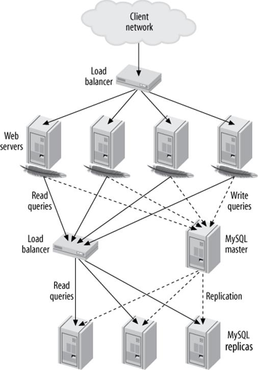
Figure 11-9. Typical load-balancing architecture for a read-intensive website
Load balancing has five common goals:
Scalability
Load balancing can help with certain kinds of scalability strategies, such as read-write splitting to read from replicas.
Efficiency
Load balancing helps you use resources more efficiently because you have control over how requests are routed. This is particularly important if your servers aren’t all equally powerful: you can direct more work to the more powerful machines.
Availability
A smart load-balancing solution uses the servers that are available at each moment.
Transparency
Clients don’t need to know about the load-balancing setup. They don’t have to care about how many machines are behind the load balancer, or what their names are; the load balancer lets the clients see a single virtual server.
Consistency
If your application is stateful (database transactions, website sessions, etc.), the load balancer should direct related requests to a single server so that the state isn’t lost between requests. This relieves the application of having to keep track of which server it’s connected to.
In the MySQL world, load-balancing architectures are often tightly coupled with sharding and replication. You can mix and match load-balancing and high-availability solutions and place them at whatever level is appropriate within your application. For example, you can load balance across multiple SQL nodes in a MySQL Cluster installation. You can also load balance across data centers, and within each data center you might have a sharded architecture, each node of which is actually part of a master-master replication pair with many replicas that are load balanced yet again. The same is true of high-availability strategies; you can have multiple levels of failover in an architecture.
Load balancing has many nuances. For example, one of the challenges is managing read/write policies. Some load-balancing technologies do this themselves, whereas others require the application to be aware of which nodes are readable and writable.
You should consider these factors when you decide how to implement load balancing. A wide variety of load-balancing solutions are available, ranging from peer-based implementations such as Wackamole (http://www.backhand.org/wackamole/) to DNS, LVS (Linux Virtual Server;http://www.linuxvirtualserver.org), hardware load balancers, TCP proxies, MySQL Proxy, and managing the load balancing in the application.
Among our customers, perhaps the most common tactic is to use hardware load balancers. Many of them use HAProxy (http://haproxy.1wt.eu), which seems to be very popular and work quite well. Some people use another TCP proxy, such as Pen (http://siag.nu/pen/). We don’t see MySQL Proxy used very often.
Connecting Directly
Some people automatically associate load balancing with a central system that’s inserted between the application and the MySQL servers. This isn’t the only way to load balance, though. You can load balance and yet still connect directly from the application to the MySQL servers. In fact, centralized load-balancing systems usually work well only when there’s a pool of servers the application can treat as interchangeable. If the application needs to make a decision such as whether it’s safe to perform a read from a replica server, it usually needs to connect directly to the server.
Besides making special-case logic possible, handling the load-balancing decisions in the application can actually be very efficient. For example, if you have two identical replicas, you can choose to use one of them for all queries that touch certain shards and the other for queries that touch other shards. This makes good use of the replicas’ memory, because each of them caches only a portion of the data from its disks in memory. And if one of the replicas fails, the other still has all the data required to serve queries to both shards.
The following sections discuss some common ways to connect directly from the application, and some of the things you should consider as you evaluate each option.
Splitting reads and writes in replication
MySQL replication gives you multiple copies of your data and lets you choose whether to run a query on the master or a replica. The primary difficulty is how to handle stale data on the replica, because replication is asynchronous. You should also treat replicas as read-only, but the master can handle both read and write queries.
You usually have to modify your application so that it’s aware of these concerns. The application can then use the master for writes and split the reads between the master and the replicas; it can use the replicas when possibly stale data doesn’t matter and use the master for data that has to be up-to-date. We call this read/write splitting.
If you use a master-master pair with an active and a passive master, the same considerations hold. In this configuration, though, only the active server should receive writes. Reads can go to the passive server if it’s OK to read potentially stale data.
The biggest problem is how to avoid artifacts caused by reading stale data. The classic artifact is when a user makes some change, such as adding a comment to a blog post, then reloads the page but doesn’t see the change because the application read stale data from a replica.
Some of the most common methods of splitting reads and writes are as follows:
Query-based split
The simplest split is to direct all writes and any reads that can never tolerate stale data to the active or master server. All other reads go to the replica or passive server. This strategy is easy to implement, but in practice it won’t use the replica as often as it could, because very few read queries can always tolerate stale data.
Stale-data split
This is a minor enhancement of the query-based split strategy. Relatively little extra work is required to make the application check the replica’s lag and decide whether or not its data is too stale to read. Many reporting applications can use this strategy: as long as the nightly data load has finished replicating to the replica, they don’t care whether it is 100% caught up with the master.
Session-based split
A slightly more sophisticated way to decide whether a read can go to a replica is to note whether the user has changed any data. The user doesn’t have to see the most up-to-date data from other users but should see her own changes. You can implement this at the session level by flagging the session as having made a change and directing the user’s read queries to the master for a certain period of time after that. This is the strategy we usually suggest to clients, because it’s a good compromise between simplicity and effectiveness.
If you want to get fancy, you can combine session-based splitting with replication lag monitoring. If the user changed some data 10 seconds ago and no replica is more than 5 seconds behind, it’s safe to read from a replica. It’s a very good idea to select one of the replicas and use it for the whole session, though, or the user might see strange effects caused by some of the replicas being farther behind than others.
Version-based split
This is similar to session-based splitting: you can track version numbers and/or timestamps for objects, and read the object’s version or timestamp from the replica to determine whether its data is fresh enough to use. If the replica’s data is too old, you can read the fresh data from the master. You can also increment the top-level item’s version number even when the object itself doesn’t change, which simplifies staleness checks (you need to look in only one place—at the top-level item). For example, you can update the user’s version if he posts a new blog entry. This will cause reads to go to the master.
Reading the object’s version from the replica adds overhead, which you can reduce with caching. We discuss caching and object versioning further in later chapters.
Global version/session split
This is a variation on version- and session-based splitting. When the application performs a write, it runs SHOW MASTER STATUS after the transaction commits. It stores the master’s log coordinates in the cache as the modified object’s and/or session’s version number. Then, when the application connects to the replica, it runs SHOW SLAVE STATUS and compares the replica’s coordinates to the stored version. If the replica has advanced to at least the point at which the master committed the transaction, the replica is safe to use for the read.
Most read/write splitting solutions require you to monitor replication lag and use it to decide where to direct reads, either in the application or through a load balancer or another man-in-the-middle system. If you do this, be aware that the Seconds_behind_master column from SHOW SLAVE STATUS is not a reliable way to monitor lag. (See Chapter 10 for details.) The pt-heartbeat tool from Percona Toolkit can help you monitor replication delay, and help maintain metadata such as binary log positions, which can ease the problems with some of the strategies we just discussed.
If you don’t care how much hardware it takes to serve your load, you can keep things simpler and not use replication for scaling reads. That might let you avoid the complexity of splitting reads between the master and replicas. Some people think this makes sense; others think it wastes hardware. This division reflects differing goals: do you want scalability only, or both scalability and efficiency? If you want efficiency too, and thus want to use the replicas for something other than just keeping a copy of the data, you’ll probably have to deal with some added complexity.
Changing the application configuration
One way you can distribute load is to reconfigure your application. For example, you can configure several machines to share the load of generating large reports. Each machine’s configuration can instruct it to connect to a different MySQL replica and generate reports for every Nth customer or site.
This system is generally very simple to implement, but if it requires any code changes—including changes to configuration files—it becomes brittle and unwieldy. Anything hardcoded that you have to change on every server, or change in a central location and “publish” via file copies or source-control update commands, is inherently limited. If you store the configuration in the database and/or a cache, you can avoid the need to publish code changes.
Changing DNS names
A crude load-balancing technique, but one that works acceptably for some simple applications, is to create DNS names for various purposes. You can then point the names at different servers as appropriate. The simplest implementation is to have one DNS name for the read-only servers and one for the writable server. If the replicas are keeping up with the master, you can change the read-only DNS name to point to the replicas; when they fall behind, you can point it back to the master.
The DNS technique is very easy to implement, but it has many drawbacks. The biggest problem is that DNS is not completely under your control:
§ DNS changes are not instantaneous or atomic. It can take a long time for DNS changes to propagate throughout a network or between networks.
§ DNS data is cached in various places, and expiry times are advisory, not mandatory.
§ DNS changes might require an application or server restart to take effect fully.
§ It’s not a good idea to use multiple IP addresses for a DNS name and rely on round-robin behavior to balance requests. The round-robin behavior isn’t always predictable.
§ The DBA might not always have direct access to DNS.
Unless the application is very simple, it’s dangerous to rely on a system that’s not controllable. You can improve your control a little by making changes to /etc/hosts instead of DNS. When you publish a change to this file, you know the change has taken effect. This is better than waiting for a cached DNS entry to expire, but it is still not ideal.
We usually advise people to build for zero reliance on DNS. It’s a good idea to avoid it even for simple applications, because you never know how large your application will grow.
Moving IP addresses
Some load-balancing solutions rely on moving virtual IP addresses[182] between servers, which can work very well. This might sound similar to making DNS changes, but it’s not the same thing. Servers don’t listen for network traffic to a DNS name; they listen for traffic to a specific IP address, so moving IP addresses allows DNS names to remain static. You can force IP address changes to be noticed very quickly and atomically via Address Resolution Protocol (ARP) commands.
The most common technology we see used for this is Pacemaker, the successor to the Linux-HA project’s Heartbeat tool. For example, you can have a single IP address associated with a role such as “read-only,” and it takes care of moving the IP address between machines as needed. Other tools for this purpose include LVS and Wackamole.
One handy technique is to assign a fixed IP address to each physical server. This IP address defines the server itself and never changes. You can then use a virtual IP address for each logical “service.” These can move between servers easily, which makes it easy to move services and application instances around without reconfiguring the application. This is a nice feature, even if you don’t move IP addresses a lot.
Introducing a Middleman
So far, the techniques we’ve discussed all assume your application is communicating directly with MySQL servers. However, many load-balancing solutions introduce a middleman whose job is to act as a proxy for the network traffic. The middleman accepts all traffic on one side and directs it to the desired server on the other, then routes the responses back to the originating machine. Sometimes the middleman is a piece of hardware, and sometimes it’s software.[183] Figure 11-10 illustrates this architecture. Such solutions generally work well, although unless you make the load balancer itself redundant, they add a single point of failure. We’ve seen a variety of load balancers used with success, from open source software such as HAProxy to pretty much any commercial system you can name.
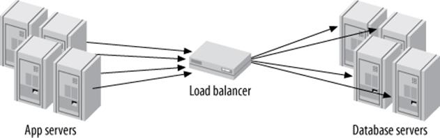
Figure 11-10. A load balancer that acts as a middleman
Load balancers
There is a wide variety of load-balancing hardware and software on the market, but few of the offerings are designed specifically for balancing load to MySQL servers.[184] Web servers need load balancing much more often, so many general-purpose load-balancing devices have special features for HTTP and only a few basic features for everything else. MySQL connections are just normal TCP/IP connections, so you can use general-purpose load balancers for MySQL. However, the lack of MySQL-specific features does add some limitations:
§ Unless the load balancer is aware of MySQL’s true load, it’s unlikely to balance load so much as distribute requests. Not all queries are equal, but general-purpose load balancers usually treat all requests as equal.
§ Most load balancers know how to inspect an HTTP request and “stick a session” to a server to preserve session state on one web server. MySQL connections are stateful too, but the load balancer is unlikely to know how to “stick” all connection requests from a single HTTP session to a single MySQL server. This results in a loss of efficiency (if a single session’s requests all go to the same MySQL server, the server’s cache will be more efficient).
§ Connection pooling and persistent connections can interfere with a load balancer’s ability to distribute connection requests. For example, suppose a connection pool opens its configured number of connections, and the load balancer distributes them among the existing four MySQL servers. Now say you add two more MySQL servers. Because the connection pool isn’t requesting any new connections, they’ll sit idle. The connections in the pool also might end up being unfairly distributed among the servers, so some are overloaded and others are underloaded. You can work around these problems by expiring the connections in the pool at various levels, but that’s complicated and difficult to do. Connection pooling solutions work best when they do their own load balancing.
§ Most general-purpose load balancers know how to do health and load checks only for HTTP servers. A simple load balancer can verify that the server accepts connections on a TCP port, which is the bare minimum. A better load balancer can make an HTTP request and check the response code to determine whether the web server is running well. MySQL doesn’t accept HTTP requests to port 3306, though, so you’ll have to build a custom health check. You can install HTTP server software on the MySQL server and point the load balancer at a custom script that actually checks the MySQL server’s status and returns an appropriate status code.[185] The most important things to check are the operating system load (generally by looking at /proc/loadavg), the replication status, and the number of MySQL connections.
Load-balancing algorithms
There are many different algorithms to determine which server should receive the next connection. Each vendor uses different terminology, but this list should provide an idea of what’s available:
Random
The load balancer directs each request to a server selected at random from the pool of available servers.
Round-robin
The load balancer sends requests to servers in a repeating sequence: A, B, C, A, B, C, etc.
Fewest connections
The next connection goes to the server with the fewest active connections.
Fastest response
The server that has been handling requests the fastest receives the next connection. This can work well when the pool contains a mix of fast and slow machines. However, it’s very tricky with SQL when the query complexity varies widely. Even the same query can perform very differently under different circumstances, such as when it’s served from the query cache or when the server’s caches already contain the needed data.
Hashed
The load balancer hashes the connection’s source IP address, which maps it to one of the servers in the pool. Each time a connection request comes from the same IP address, the load balancer sends it to the same server. The bindings change only when the number of machines in the pool does.
Weighted
The load balancer can combine and weight several of the other algorithms. For example, you might have single- and dual-CPU machines. The dual-CPU machines are roughly twice as powerful, so you can tell the load balancer to send them an average of twice as many requests.
The best algorithm for MySQL depends on your workload. The least-connections algorithm, for example, might flood new servers when you add them to the pool of available servers—before when their caches are warmed up. The authors of this book’s first edition experienced that problem firsthand.
You’ll need to experiment to find the best performance for your workload. Be sure to consider what happens in extraordinary circumstances as well as in the day-to-day norm. It is in those extraordinary circumstances—e.g., during times of high load, when you’re doing schema changes, or when an unusual number of servers go offline—that you can least afford something going terribly wrong.
We’ve described only instant-provisioning algorithms here, which don’t queue connection requests. Sometimes algorithms that use queuing can be more efficient. For example, an algorithm might maintain a given concurrency on the database server, such as allowing no more than N active transactions at the same time. If there are too many active transactions, the algorithm can put a new request in a queue and serve it from the first server that becomes “available” according to the criteria. Some connection pools support queuing algorithms.
Adding and removing servers in the pool
Adding a new server to the pool is usually not as simple as plugging it in and notifying the load balancer of its existence. You might think it’ll be OK as long as it doesn’t get flooded with connections, but that’s not always true. Sometimes you can add load to a server slowly, but some servers whose caches are cold might be so slow that they shouldn’t get any user queries for a while. If it takes 30 seconds to return the data a user needs to see for a page view, the server is unusable even for a small amount of traffic. You can avoid this problem by mirroring SELECT traffic from an active server for a while before you notify the load balancer about the new server. You can do this by reading and replaying the active server’s log files on the newly started server, or by capturing the production server’s network traffic and replaying a portion of its queries. The pt-query-digesttool from Percona Toolkit can help with this. Another tactic that can work well is to use the fast warmup features in Percona Server or MySQL 5.6.
You should configure the servers in the connection pool so that there is enough unused capacity to let you take servers out for maintenance, or to handle the load when servers fail. You need more than just “enough” capacity on each server.
Make sure your configuration limits are high enough to work when servers are out of the pool. For example, if you find that each MySQL server typically has 100 connections, you should set max_connections to 200 on each server in the pool. Then, even if half the servers fail, the pool should be able to handle the same number of connections as a whole.
Load Balancing with a Master and Multiple Replicas
The most common replication topology is a single master with multiple replicas. It can be difficult to move away from this architecture. Many applications assume there’s a single destination for all writes, or that all data will always be available on a single server. Though this is not the most scalable architecture, there are ways you can use it to good effect with load balancing. This section examines some of those techniques:
Functional partitioning
You can stretch capacity quite a bit by configuring replicas or groups of replicas for particular purposes, as discussed previously. Common functions you might consider separating are reporting and analytics, data warehousing, and full-text searching. You can find more ideas inChapter 10.
Filtering and data partitioning
You can partition data among otherwise similar replicas with replication filters (see Chapter 10). This strategy can work well as long as your data is already separated into different databases or tables on the master. Unfortunately, there’s no built-in way to filter replication at the level of individual rows. You’d have to do something creative (read: hackish) to accomplish this, perhaps with triggers and a bunch of different tables.
Even if you don’t partition the data amongst the replicas, you can improve cache efficiency by partitioning reads instead of distributing them randomly. For instance, you might direct all reads for users whose names begin with the letters A–M to a given replica, and all reads for users whose names begin with N–Z to another replica. This helps use each machine’s cache more fully, because repeated reads are more likely to find the relevant data in the cache. In the best case, where there are no writes, this strategy effectively gives you a total cache size the same as the two machines’ cache sizes combined. In comparison, if you distribute the reads randomly among the replicas, every machine’s cache essentially duplicates the data, and your total effective cache size is only as big as a single replica’s cache, no matter how many replicas you have.
Moving parts of writes to a replica
The master doesn’t always have to do all the work involved in writes. You can save a significant amount of redundant work for the master and the replicas by decomposing write queries and running parts of them on replicas. See Chapter 10 for more on this topic.
Guaranteeing a replica is caught up
If you want to run a certain process on the replica, and it needs to know that its data is current as of a certain point in time—even if it has to wait a while for that to happen—you can use the MASTER_POS_WAIT() function to block until the replica catches up to the desired point on the master. Alternatively, you can use a replication heartbeat to check for up-to-dateness; see Chapter 10 for more on this.
Write synchronization
You can also use MASTER_POS_WAIT() to make sure your writes actually reach one or more replicas. If your application needs to emulate synchronous replication to guarantee data safety, it can cycle between each replica, running MASTER_POS_WAIT() on each. This creates a “synchronization barrier” that can take a long time to pass if any of the replicas is far behind in replication, so it’s a good idea to use it only when absolutely necessary. (You can also wait until just one replica receives the event if your goal is only to ensure that some replica has the event. MySQL 5.5 adds semisynchronous replication, which supports this technique natively.)
[182] Virtual IP addresses aren’t connected to any specific computer or network interfaces; they “float” between computers.
[183] You can configure some solutions such as LVS so they are involved only when an application needs to create a new connection, and don’t act as a middleman after that.
[184] MySQL Proxy is an exception, but it hasn’t proved to work all that well in the field, due to problems such as added latency and scalability bottlenecks.
[185] Actually, if your coding kung fu is up to the task of writing a program to listen on port 80, or if you configure xinetd to invoke your program, you don’t even need to install a web server.
Summary
Scaling MySQL correctly is a bit less glamorous than it often seems. The right way to scale isn’t to build the next Facebook architecture from day one. A better strategy is to do what’s clearly needed for your application, and plan ahead so that if you do grow very rapidly, your success will finance whatever steps are necessary to meet the demand.
It is valuable to have a mathematical definition of scalability, just as it’s useful to have a precise concept of performance, and the Universal Scalability Law can provide a helpful framework. Knowing that systems fail to scale linearly because of costs such as serialization and crosstalk can help you avoid building those problems into your application. At the same time, many scalability problems aren’t mathematical; they may be due to problems within the organization, such as lack of teamwork or other less concrete issues. Dr. Neil J. Gunther’s book Guerrilla Capacity Planning and Eliyahu M. Goldratt’s book The Goal are good reading for anyone interested in understanding more about why systems don’t scale.
In terms of MySQL scalability strategies, the typical application that grows very large usually moves from a single server, to a scale-out architecture with read replicas, to sharding and/or functional partitioning. We disagree with those who advocate a “shard early, shard often” approach for every application. It’s complicated and expensive, and many applications will never need it. It is perfectly legitimate to bide your time and see what happens with new hardware, new versions of MySQL, or new developments in MySQL Cluster, and even to evaluate a proprietary system such as Clustrix. Sharding is a hand-built clustering system, after all, and it’s a good idea not to reinvent the wheel if you don’t need to.
Where there are multiple servers, there are problems with consistency and atomicity. The most common problems we see are lack of session consistency (posting a comment on a website, refreshing the page, and not seeing the comment you just posted) and failures when telling the application which servers are readable and writable. The latter are much more serious, because if you direct writes to more than one place in your application you’ll inevitably end up with data problems, which can be amazingly difficult and time-consuming to solve. Load balancers can help with this, but load balancers can also create problems of their own, sometimes even aggravating the problems they’re intended to help solve. This is why our next chapter is on high availability.
All materials on the site are licensed Creative Commons Attribution-Sharealike 3.0 Unported CC BY-SA 3.0 & GNU Free Documentation License (GFDL)
If you are the copyright holder of any material contained on our site and intend to remove it, please contact our site administrator for approval.
© 2016-2026 All site design rights belong to S.Y.A.