High Performance MySQL (2012)
Chapter 6. Query Performance Optimization
In the previous chapters we explained schema optimization and indexing, which are necessary for high performance. But they aren’t enough—you also need to design your queries well. If your queries are bad, even the best-designed schema and indexes will not perform well.
Query optimization, index optimization, and schema optimization go hand in hand. As you gain experience writing queries in MySQL, you will learn how to design tables and indexes to support efficient queries. Similarly, what you learn about optimal schema design will influence the kinds of queries you write. This process takes time, so we encourage you to refer back to these three chapters as you learn more.
This chapter begins with general query design considerations—the things you should consider first when a query isn’t performing well. We then dig much deeper into query optimization and server internals. We show you how to find out how MySQL executes a particular query, and you’ll learn how to change the query execution plan. Finally, we’ll look at some places MySQL doesn’t optimize queries well and explore query optimization patterns that help MySQL execute queries more efficiently.
Our goal is to help you understand deeply how MySQL really executes queries, so you can reason about what is efficient or inefficient, exploit MySQL’s strengths, and avoid its weaknesses.
Why Are Queries Slow?
Before trying to write fast queries, remember that it’s all about response time. Queries are tasks, but they are composed of subtasks, and those subtasks consume time. To optimize a query, you must optimize its subtasks by eliminating them, making them happen fewer times, or making them happen more quickly.[69]
What are the subtasks that MySQL performs to execute a query, and which ones are slow? The full list is impossible to include here, but if you profile a query as we showed in Chapter 3, you will find out what tasks it performs. In general, you can think of a query’s lifetime by mentally following the query through its sequence diagram from the client to the server, where it is parsed, planned, and executed, and then back again to the client. Execution is one of the most important stages in a query’s lifetime. It involves lots of calls to the storage engine to retrieve rows, as well as post-retrieval operations such as grouping and sorting.
While accomplishing all these tasks, the query spends time on the network, in the CPU, in operations such as statistics and planning, locking (mutex waits), and most especially, calls to the storage engine to retrieve rows. These calls consume time in memory operations, CPU operations, and especially I/O operations if the data isn’t in memory. Depending on the storage engine, a lot of context switching and/or system calls might also be involved.
In every case, excessive time may be consumed because the operations are performed needlessly, performed too many times, or are too slow. The goal of optimization is to avoid that, by eliminating or reducing operations, or making them faster.
Again, this isn’t a complete or accurate picture of a query’s life. Our goal here is to show the importance of understanding a query’s lifecycle and thinking in terms of where the time is consumed. With that in mind, let’s see how to optimize queries.
[69] Sometimes you might also need to modify a query to reduce its impact on other queries running on the system. In this case, you’re trying to reduce the query’s resource consumption, a topic we discussed in Chapter 3.
Slow Query Basics: Optimize Data Access
The most basic reason a query doesn’t perform well is because it’s working with too much data. Some queries just have to sift through a lot of data and can’t be helped. That’s unusual, though; most bad queries can be changed to access less data. We’ve found it useful to analyze a poorly performing query in two steps:
1. Find out whether your application is retrieving more data than you need. That usually means it’s accessing too many rows, but it might also be accessing too many columns.
2. Find out whether the MySQL server is analyzing more rows than it needs.
Are You Asking the Database for Data You Don’t Need?
Some queries ask for more data than they need and then throw some of it away. This demands extra work of the MySQL server, adds network overhead,[70] and consumes memory and CPU resources on the application server.
Here are a few typical mistakes:
Fetching more rows than needed
One common mistake is assuming that MySQL provides results on demand, rather than calculating and returning the full result set. We often see this in applications designed by people familiar with other database systems. These developers are used to techniques such as issuing a SELECTstatement that returns many rows, then fetching the first N rows and closing the result set (e.g., fetching the 100 most recent articles for a news site when they only need to show 10 of them on the front page). They think MySQL will provide them with these 10 rows and stop executing the query, but what MySQL really does is generate the complete result set. The client library then fetches all the data and discards most of it. The best solution is to add a LIMIT clause to the query.
Fetching all columns from a multitable join
If you want to retrieve all actors who appear in the film Academy Dinosaur, don’t write the query this way:
mysql> SELECT * FROM sakila.actor
-> INNER JOIN sakila.film_actor USING(actor_id)
-> INNER JOIN sakila.film USING(film_id)
-> WHERE sakila.film.title = 'Academy Dinosaur';
That returns all columns from all three tables. Instead, write the query as follows:
mysql> SELECT sakila.actor.* FROM sakila.actor...;
Fetching all columns
You should always be suspicious when you see SELECT *. Do you really need all columns? Probably not. Retrieving all columns can prevent optimizations such as covering indexes, as well as adding I/O, memory, and CPU overhead for the server.
Some DBAs ban SELECT * universally because of this fact, and to reduce the risk of problems when someone alters the table’s column list.
Of course, asking for more data than you really need is not always bad. In many cases we’ve investigated, people tell us the wasteful approach simplifies development, because it lets the developer use the same bit of code in more than one place. That’s a reasonable consideration, as long as you know what it costs in terms of performance. It might also be useful to retrieve more data than you actually need if you use some type of caching in your application, or if you have another benefit in mind. Fetching and caching full objects might be preferable to running many separate queries that retrieve only parts of the object.
Fetching the same data repeatedly
If you’re not careful, it’s quite easy to write application code that retrieves the same data repeatedly from the database server, executing the same query to fetch it. For example, if you want to find out a user’s profile image URL to display next to a list of comments, you might request this repeatedly for each comment. Or you could cache it the first time you fetch it, and reuse it thereafter. The latter approach is much more efficient.
Is MySQL Examining Too Much Data?
Once you’re sure your queries retrieve only the data you need, you can look for queries that examine too much data while generating results. In MySQL, the simplest query cost metrics are:
§ Response time
§ Number of rows examined
§ Number of rows returned
None of these metrics is a perfect way to measure query cost, but they reflect roughly how much data MySQL must access internally to execute a query and translate approximately into how fast the query runs. All three metrics are logged in the slow query log, so looking at the slow query log is one of the best ways to find queries that examine too much data.
Response time
Beware of taking query response time at face value. Hey, isn’t that the opposite of what we’ve been telling you? Not really. It’s still true that response time is what matters, but it’s a bit complicated.
Response time is the sum of two things: service time and queue time. Service time is how long it takes the server to actually process the query. Queue time is the portion of response time during which the server isn’t really executing the query—it’s waiting for something, such as waiting for an I/O operation to complete, waiting for a row lock, and so forth. The problem is, you can’t break the response time down into these components unless you can measure them individually, which is usually hard to do. In general, the most common and important waits you’ll encounter are I/O and lock waits, but you shouldn’t count on that, because it varies a lot.
As a result, response time is not consistent under varying load conditions. Other factors—such as storage engine locks (table locks and row locks), high concurrency, and hardware—can also have a considerable impact on response times. Response time can also be both a symptom and a cause of problems, and it’s not always obvious which is the case, unless you can use the techniques shown in Single-Query Versus Server-Wide Problems to find out.
When you look at a query’s response time, you should ask yourself whether the response time is reasonable for the query. We don’t have space for a detailed explanation in this book, but you can actually calculate a quick upper-bound estimate (QUBE) of query response time using the techniques explained in Tapio Lahdenmaki and Mike Leach’s book Relational Database Index Design and the Optimizers (Wiley). In a nutshell: examine the query execution plan and the indexes involved, determine how many sequential and random I/O operations might be required, and multiply these by the time it takes your hardware to perform them. Add it all up and you have a yardstick to judge whether a query is slower than it could or should be.
Rows examined and rows returned
It’s useful to think about the number of rows examined when analyzing queries, because you can see how efficiently the queries are finding the data you need.
However, this is not a perfect metric for finding “bad” queries. Not all row accesses are equal. Shorter rows are faster to access, and fetching rows from memory is much faster than reading them from disk.
Ideally, the number of rows examined would be the same as the number returned, but in practice this is rarely possible. For example, when constructing rows with joins, the server must access multiple rows to generate each row in the result set. The ratio of rows examined to rows returned is usually small—say, between 1:1 and 10:1—but sometimes it can be orders of magnitude larger.
Rows examined and access types
When you’re thinking about the cost of a query, consider the cost of finding a single row in a table. MySQL can use several access methods to find and return a row. Some require examining many rows, but others might be able to generate the result without examining any.
The access method(s) appear in the type column in EXPLAIN’s output. The access types range from a full table scan to index scans, range scans, unique index lookups, and constants. Each of these is faster than the one before it, because it requires reading less data. You don’t need to memorize the access types, but you should understand the general concepts of scanning a table, scanning an index, range accesses, and single-value accesses.
If you aren’t getting a good access type, the best way to solve the problem is usually by adding an appropriate index. We discussed indexing in the previous chapter; now you can see why indexes are so important to query optimization. Indexes let MySQL find rows with a more efficient access type that examines less data.
For example, let’s look at a simple query on the Sakila sample database:
mysql> SELECT * FROM sakila.film_actor WHERE film_id = 1;
This query will return 10 rows, and EXPLAIN shows that MySQL uses the ref access type on the idx_fk_film_id index to execute the query:
mysql> EXPLAIN SELECT * FROM sakila.film_actor WHERE film_id = 1\G
*************************** 1. row ***************************
id: 1
select_type: SIMPLE
table: film_actor
type: ref
possible_keys: idx_fk_film_id
key: idx_fk_film_id
key_len: 2
ref: const
rows: 10
Extra:
EXPLAIN shows that MySQL estimated it needed to access only 10 rows. In other words, the query optimizer knew the chosen access type could satisfy the query efficiently. What would happen if there were no suitable index for the query? MySQL would have to use a less optimal access type, as we can see if we drop the index and run the query again:
mysql> ALTER TABLE sakila.film_actor DROP FOREIGN KEY fk_film_actor_film;
mysql> ALTER TABLE sakila.film_actor DROP KEY idx_fk_film_id;
mysql> EXPLAIN SELECT * FROM sakila.film_actor WHERE film_id = 1\G
*************************** 1. row ***************************
id: 1
select_type: SIMPLE
table: film_actor
type: ALL
possible_keys: NULL
key: NULL
key_len: NULL
ref: NULL
rows: 5073
Extra: Using where
Predictably, the access type has changed to a full table scan (ALL), and MySQL now estimates it’ll have to examine 5,073 rows to satisfy the query. The “Using where” in the Extra column shows that the MySQL server is using the WHERE clause to discard rows after the storage engine reads them.
In general, MySQL can apply a WHERE clause in three ways, from best to worst:
§ Apply the conditions to the index lookup operation to eliminate nonmatching rows. This happens at the storage engine layer.
§ Use a covering index (“Using index” in the Extra column) to avoid row accesses, and filter out nonmatching rows after retrieving each result from the index. This happens at the server layer, but it doesn’t require reading rows from the table.
§ Retrieve rows from the table, then filter nonmatching rows (“Using where” in the Extra column). This happens at the server layer and requires the server to read rows from the table before it can filter them.
This example illustrates how important it is to have good indexes. Good indexes help your queries get a good access type and examine only the rows they need. However, adding an index doesn’t always mean that MySQL will access and return the same number of rows. For example, here’s a query that uses the COUNT() aggregate function:[71]
mysql> SELECT actor_id, COUNT(*) FROM sakila.film_actor GROUP BY actor_id;
This query returns only 200 rows, but it needs to read thousands of rows to build the result set. An index can’t reduce the number of rows examined for a query like this one.
Unfortunately, MySQL does not tell you how many of the rows it accessed were used to build the result set; it tells you only the total number of rows it accessed. Many of these rows could be eliminated by a WHERE clause and end up not contributing to the result set. In the previous example, after removing the index on sakila.film_actor, the query accessed every row in the table and the WHERE clause discarded all but 10 of them. Only the remaining 10 rows were used to build the result set. Understanding how many rows the server accesses and how many it really uses requires reasoning about the query.
If you find that a huge number of rows were examined to produce relatively few rows in the result, you can try some more sophisticated fixes:
§ Use covering indexes, which store data so that the storage engine doesn’t have to retrieve the complete rows. (We discussed these in the previous chapter.)
§ Change the schema. An example is using summary tables (discussed in Chapter 4).
§ Rewrite a complicated query so the MySQL optimizer is able to execute it optimally. (We discuss this later in this chapter.)
[70] Network overhead is worst if the application is on a different host from the server, but transferring data between MySQL and the application isn’t free even if they’re on the same server.
[71] See Optimizing COUNT() Queries for more on this topic.
Ways to Restructure Queries
As you optimize problematic queries, your goal should be to find alternative ways to get the result you want—but that doesn’t necessarily mean getting the same result set back from MySQL. You can sometimes transform queries into equivalent forms that return the same results, and get better performance. However, you should also think about rewriting the query to retrieve different results, if that provides an efficiency benefit. You might be able to ultimately do the same work by changing the application code as well as the query. In this section, we explain techniques that can help you restructure a wide range of queries and show you when to use each technique.
Complex Queries Versus Many Queries
One important query design question is whether it’s preferable to break up a complex query into several simpler queries. The traditional approach to database design emphasizes doing as much work as possible with as few queries as possible. This approach was historically better because of the cost of network communication and the overhead of the query parsing and optimization stages.
However, this advice doesn’t apply as much to MySQL, because it was designed to handle connecting and disconnecting very efficiently and to respond to small and simple queries very quickly. Modern networks are also significantly faster than they used to be, reducing network latency. Depending on the server version, MySQL can run well over 100,000 simple queries per second on commodity server hardware and over 2,000 queries per second from a single correspondent on a gigabit network, so running multiple queries isn’t necessarily such a bad thing.
Connection response is still slow compared to the number of rows MySQL can traverse per second internally, though, which is counted in millions per second for in-memory data. All else being equal, it’s still a good idea to use as few queries as possible, but sometimes you can make a query more efficient by decomposing it and executing a few simple queries instead of one complex one. Don’t be afraid to do this; weigh the costs, and go with the strategy that causes less work. We show some examples of this technique a little later in the chapter.
That said, using too many queries is a common mistake in application design. For example, some applications perform 10 single-row queries to retrieve data from a table when they could use a single 10-row query. We’ve even seen applications that retrieve each column individually, querying each row many times!
Chopping Up a Query
Another way to slice up a query is to divide and conquer, keeping it essentially the same but running it in smaller “chunks” that affect fewer rows each time.
Purging old data is a great example. Periodic purge jobs might need to remove quite a bit of data, and doing this in one massive query could lock a lot of rows for a long time, fill up transaction logs, hog resources, and block small queries that shouldn’t be interrupted. Chopping up theDELETE statement and using medium-size queries can improve performance considerably, and reduce replication lag when a query is replicated. For example, instead of running this monolithic query:
mysql> DELETE FROM messages WHERE created < DATE_SUB(NOW(),INTERVAL 3 MONTH);
you could do something like the following pseudocode:
rows_affected = 0
do {
rows_affected = do_query(
"DELETE FROM messages WHERE created < DATE_SUB(NOW(),INTERVAL 3 MONTH)
LIMIT 10000")
} while rows_affected > 0
Deleting 10,000 rows at a time is typically a large enough task to make each query efficient, and a short enough task to minimize the impact on the server[72] (transactional storage engines might benefit from smaller transactions). It might also be a good idea to add some sleep time between theDELETE statements to spread the load over time and reduce the amount of time locks are held.
Join Decomposition
Many high-performance applications use join decomposition. You can decompose a join by running multiple single-table queries instead of a multitable join, and then performing the join in the application. For example, instead of this single query:
mysql> SELECT * FROM tag
-> JOIN tag_post ON tag_post.tag_id=tag.id
-> JOIN post ON tag_post.post_id=post.id
-> WHERE tag.tag='mysql';
You might run these queries:
mysql> SELECT * FROM tag WHERE tag='mysql';
mysql> SELECT * FROM tag_post WHERE tag_id=1234;
mysql> SELECT * FROM post WHERE post.id in (123,456,567,9098,8904);
Why on earth would you do this? It looks wasteful at first glance, because you’ve increased the number of queries without getting anything in return. However, such restructuring can actually give significant performance advantages:
§ Caching can be more efficient. Many applications cache “objects” that map directly to tables. In this example, if the object with the tag mysql is already cached, the application can skip the first query. If you find posts with an ID of 123, 567, or 9098 in the cache, you can remove them from the IN() list. The query cache might also benefit from this strategy. If only one of the tables changes frequently, decomposing a join can reduce the number of cache invalidations.
§ Executing the queries individually can sometimes reduce lock contention.
§ Doing joins in the application makes it easier to scale the database by placing tables on different servers.
§ The queries themselves can be more efficient. In this example, using an IN() list instead of a join lets MySQL sort row IDs and retrieve rows more optimally than might be possible with a join. We explain this in more detail later.
§ You can reduce redundant row accesses. Doing a join in the application means you retrieve each row only once, whereas a join in the query is essentially a denormalization that might repeatedly access the same data. For the same reason, such restructuring might also reduce the total network traffic and memory usage.
§ To some extent, you can view this technique as manually implementing a hash join instead of the nested loops algorithm MySQL uses to execute a join. A hash join might be more efficient. (We discuss MySQL’s join strategy later in this chapter.)
As a result, doing joins in the application can be more efficient when you cache and reuse a lot of data from earlier queries, you distribute data across multiple servers, you replace joins with IN() lists on large tables, or a join refers to the same table multiple times.
[72] Percona Toolkit’s pt-archiver tool makes these types of jobs easy and safe.
Query Execution Basics
If you need to get high performance from your MySQL server, one of the best ways to invest your time is in learning how MySQL optimizes and executes queries. Once you understand this, much of query optimization is a matter of reasoning from principles, and query optimization becomes a very logical process.
In other words, it’s time to revisit what we discussed earlier: the process MySQL follows to execute queries. Follow along with Figure 6-1 to see what happens when you send MySQL a query:
1. The client sends the SQL statement to the server.
2. The server checks the query cache. If there’s a hit, it returns the stored result from the cache; otherwise, it passes the SQL statement to the next step.
3. The server parses, preprocesses, and optimizes the SQL into a query execution plan.
4. The query execution engine executes the plan by making calls to the storage engine API.
5. The server sends the result to the client.
Each of these steps has some extra complexity, which we discuss in the following sections. We also explain which states the query will be in during each step. The query optimization process is particularly complex and important to understand. There are also exceptions or special cases, such as the difference in execution path when you use prepared statements; we discuss that in the next chapter.
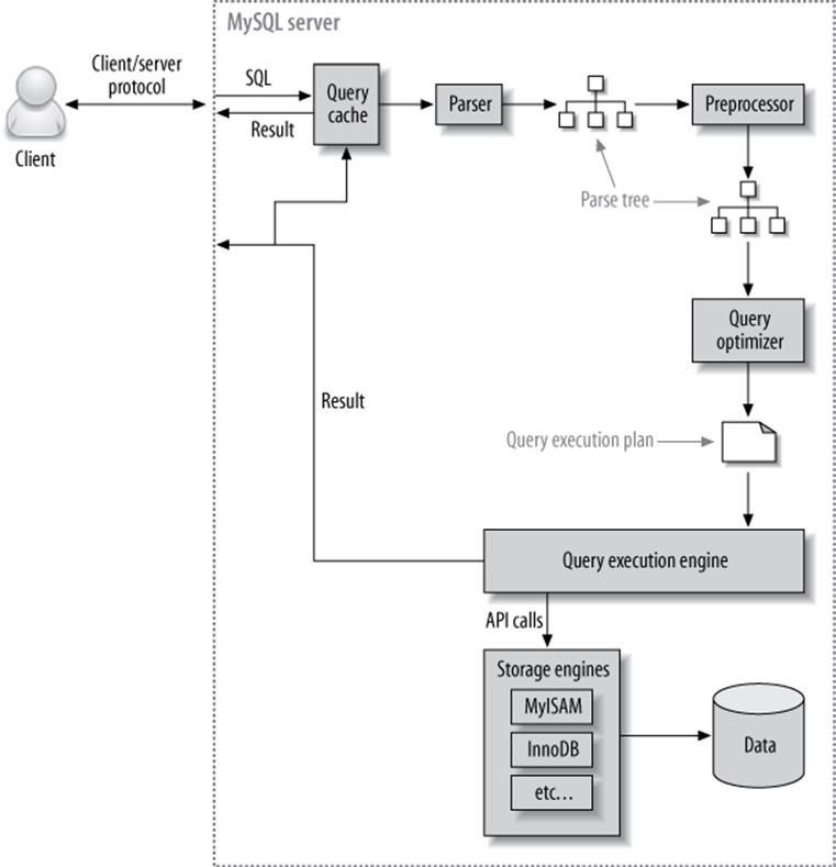
Figure 6-1. Execution path of a query
The MySQL Client/Server Protocol
Though you don’t need to understand the inner details of MySQL’s client/server protocol, you do need to understand how it works at a high level. The protocol is half-duplex, which means that at any given time the MySQL server can be either sending or receiving messages, but not both. It also means there is no way to cut a message short.
This protocol makes MySQL communication simple and fast, but it limits it in some ways too. For one thing, it means there’s no flow control; once one side sends a message, the other side must fetch the entire message before responding. It’s like a game of tossing a ball back and forth: only one side has the ball at any instant, and you can’t toss the ball (send a message) unless you have it.
The client sends a query to the server as a single packet of data. This is why the max_allowed_packet configuration variable is important if you have large queries.[73] Once the client sends the query, it doesn’t have the ball anymore; it can only wait for results.
In contrast, the response from the server usually consists of many packets of data. When the server responds, the client has to receive the entire result set. It cannot simply fetch a few rows and then ask the server not to bother sending the rest. If the client needs only the first few rows that are returned, it either has to wait for all of the server’s packets to arrive and then discard the ones it doesn’t need, or disconnect ungracefully. Neither is a good idea, which is why appropriate LIMIT clauses are so important.
Here’s another way to think about this: when a client fetches rows from the server, it thinks it’s pulling them. But the truth is, the MySQL server is pushing the rows as it generates them. The client is only receiving the pushed rows; there is no way for it to tell the server to stop sending rows. The client is “drinking from the fire hose,” so to speak. (Yes, that’s a technical term.)
Most libraries that connect to MySQL let you either fetch the whole result set and buffer it in memory, or fetch each row as you need it. The default behavior is generally to fetch the whole result and buffer it in memory. This is important because until all the rows have been fetched, the MySQL server will not release the locks and other resources required by the query. The query will be in the “Sending data” state. When the client library fetches the results all at once, it reduces the amount of work the server needs to do: the server can finish and clean up the query as quickly as possible.
Most client libraries let you treat the result set as though you’re fetching it from the server, although in fact you’re just fetching it from the buffer in the library’s memory. This works fine most of the time, but it’s not a good idea for huge result sets that might take a long time to fetch and use a lot of memory. You can use less memory, and start working on the result sooner, if you instruct the library not to buffer the result. The downside is that the locks and other resources on the server will remain open while your application is interacting with the library.[74]
Let’s look at an example using PHP. First, here’s how you’ll usually query MySQL from PHP:
<?php
$link = mysql_connect('localhost', 'user', 'p4ssword');
$result = mysql_query('SELECT * FROM HUGE_TABLE', $link);
while ( $row = mysql_fetch_array($result) ) {
// Do something with result
}
?>
The code seems to indicate that you fetch rows only when you need them, in the while loop. However, the code actually fetches the entire result into a buffer with the mysql_query() function call. The while loop simply iterates through the buffer. In contrast, the following code doesn’t buffer the results, because it uses mysql_unbuffered_query() instead of mysql_query():
<?php
$link = mysql_connect('localhost', 'user', 'p4ssword');
$result = mysql_unbuffered_query('SELECT * FROM HUGE_TABLE', $link);
while ( $row = mysql_fetch_array($result) ) {
// Do something with result
}
?>
Programming languages have different ways to override buffering. For example, the Perl DBD::mysql driver requires you to specify the C client library’s mysql_use_result attribute (the default is mysql_buffer_result). Here’s an example:
#!/usr/bin/perl
use DBI;
my $dbh = DBI->connect('DBI:mysql:;host=localhost', 'user', 'p4ssword');
my $sth = $dbh->prepare('SELECT * FROM HUGE_TABLE', { mysql_use_result => 1 });
$sth->execute();
while ( my $row = $sth->fetchrow_array() ) {
# Do something with result
}
Notice that the call to prepare() specified to “use” the result instead of “buffering” it. You can also specify this when connecting, which will make every statement unbuffered:
my $dbh = DBI->connect('DBI:mysql:;mysql_use_result=1', 'user', 'p4ssword');
Query states
Each MySQL connection, or thread, has a state that shows what it is doing at any given time. There are several ways to view these states, but the easiest is to use the SHOW FULL PROCESSLIST command (the states appear in the Command column). As a query progresses through its lifecycle, its state changes many times, and there are dozens of states. The MySQL manual is the authoritative source of information for all the states, but we list a few here and explain what they mean:
Sleep
The thread is waiting for a new query from the client.
Query
The thread is either executing the query or sending the result back to the client.
Locked
The thread is waiting for a table lock to be granted at the server level. Locks that are implemented by the storage engine, such as InnoDB’s row locks, do not cause the thread to enter the Locked state. This thread state is the classic symptom of MyISAM locking, but it can occur in other storage engines that don’t have row-level locking, too.
Analyzing and statistics
The thread is checking storage engine statistics and optimizing the query.
Copying to tmp table [on disk]
The thread is processing the query and copying results to a temporary table, probably for a GROUP BY, for a filesort, or to satisfy a UNION. If the state ends with “on disk,” MySQL is converting an in-memory table to an on-disk table.
Sorting result
The thread is sorting a result set.
Sending data
This can mean several things: the thread might be sending data between stages of the query, generating the result set, or returning the result set to the client.
It’s helpful to at least know the basic states, so you can get a sense of “who has the ball” for the query. On very busy servers, you might see an unusual or normally brief state, such as statistics, begin to take a significant amount of time. This usually indicates that something is wrong, and you should use the techniques shown in Chapter 3 to capture detailed diagnostic data when it happens.
The Query Cache
Before even parsing a query, MySQL checks for it in the query cache, if the cache is enabled. This operation is a case-sensitive hash lookup. If the query differs from a similar query in the cache by even a single byte, it won’t match,[75] and the query processing will go to the next stage.
If MySQL does find a match in the query cache, it must check privileges before returning the cached query. This is possible without parsing the query, because MySQL stores table information with the cached query. If the privileges are OK, MySQL retrieves the stored result from the query cache and sends it to the client, bypassing every other stage in query execution. The query is never parsed, optimized, or executed.
You can learn more about the query cache in Chapter 7.
The Query Optimization Process
The next step in the query lifecycle turns a SQL query into an execution plan for the query execution engine. It has several substeps: parsing, preprocessing, and optimization. Errors (for example, syntax errors) can be raised at any point in the process. We’re not trying to document the MySQL internals here, so we’re going to take some liberties, such as describing steps separately even though they’re often combined wholly or partially for efficiency. Our goal is simply to help you understand how MySQL executes queries so that you can write better ones.
The parser and the preprocessor
To begin, MySQL’s parser breaks the query into tokens and builds a “parse tree” from them. The parser uses MySQL’s SQL grammar to interpret and validate the query. For instance, it ensures that the tokens in the query are valid and in the proper order, and it checks for mistakes such as quoted strings that aren’t terminated.
The preprocessor then checks the resulting parse tree for additional semantics that the parser can’t resolve. For example, it checks that tables and columns exist, and it resolves names and aliases to ensure that column references aren’t ambiguous.
Next, the preprocessor checks privileges. This is normally very fast unless your server has large numbers of privileges.
The query optimizer
The parse tree is now valid and ready for the optimizer to turn it into a query execution plan. A query can often be executed many different ways and produce the same result. The optimizer’s job is to find the best option.
MySQL uses a cost-based optimizer, which means it tries to predict the cost of various execution plans and choose the least expensive. The unit of cost was originally a single random 4 KB data page read, but it has become more sophisticated and now includes factors such as the estimated cost of executing a WHERE clause comparison. You can see how expensive the optimizer estimated a query to be by running the query, then inspecting the Last_query_cost session variable:
mysql> SELECT SQL_NO_CACHE COUNT(*) FROM sakila.film_actor;
+----------+
| count(*) |
+----------+
| 5462 |
+----------+
mysql> SHOW STATUS LIKE 'Last_query_cost';
+-----------------+-------------+
| Variable_name | Value |
+-----------------+-------------+
| Last_query_cost | 1040.599000 |
+-----------------+-------------+
This result means that the optimizer estimated it would need to do about 1,040 random data page reads to execute the query. It bases the estimate on statistics: the number of pages per table or index, the cardinality (number of distinct values) of the indexes, the length of the rows and keys, and the key distribution. The optimizer does not include the effects of any type of caching in its estimates—it assumes every read will result in a disk I/O operation.
The optimizer might not always choose the best plan, for many reasons:
§ The statistics could be wrong. The server relies on storage engines to provide statistics, and they can range from exactly correct to wildly inaccurate. For example, the InnoDB storage engine doesn’t maintain accurate statistics about the number of rows in a table because of its MVCC architecture.
§ The cost metric is not exactly equivalent to the true cost of running the query, so even when the statistics are accurate, the query might be more or less expensive than MySQL’s approximation. A plan that reads more pages might actually be cheaper in some cases, such as when the reads are sequential so the disk I/O is faster, or when the pages are already cached in memory. MySQL also doesn’t understand which pages are in memory and which pages are on disk, so it doesn’t really know how much I/O the query will cause.
§ MySQL’s idea of “optimal” might not match yours. You probably want the fastest execution time, but MySQL doesn’t really try to make queries fast; it tries to minimize their cost, and as we’ve seen, determining cost is not an exact science.
§ MySQL doesn’t consider other queries that are running concurrently, which can affect how quickly the query runs.
§ MySQL doesn’t always do cost-based optimization. Sometimes it just follows the rules, such as “if there’s a full-text MATCH() clause, use a FULLTEXT index if one exists.” It will do this even when it would be faster to use a different index and a non-FULLTEXT query with a WHEREclause.
§ The optimizer doesn’t take into account the cost of operations not under its control, such as executing stored functions or user-defined functions.
§ As we’ll see later, the optimizer can’t always estimate every possible execution plan, so it might miss an optimal plan.
MySQL’s query optimizer is a highly complex piece of software, and it uses many optimizations to transform the query into an execution plan. There are two basic types of optimizations, which we call static and dynamic. Static optimizations can be performed simply by inspecting the parse tree. For example, the optimizer can transform the WHERE clause into an equivalent form by applying algebraic rules. Static optimizations are independent of values, such as the value of a constant in a WHERE clause. They can be performed once and will always be valid, even when the query is reexecuted with different values. You can think of these as “compile-time optimizations.”
In contrast, dynamic optimizations are based on context and can depend on many factors, such as which value is in a WHERE clause or how many rows are in an index. They must be reevaluated each time the query is executed. You can think of these as “runtime optimizations.”
The difference is important when executing prepared statements or stored procedures. MySQL can do static optimizations once, but it must reevaluate dynamic optimizations every time it executes a query. MySQL sometimes even reoptimizes the query as it executes it.[76]
Here are some types of optimizations MySQL knows how to do:
Reordering joins
Tables don’t always have to be joined in the order you specify in the query. Determining the best join order is an important optimization; we explain it in depth later in this chapter.
Converting OUTER JOINs to INNER JOINs
An OUTER JOIN doesn’t necessarily have to be executed as an OUTER JOIN. Some factors, such as the WHERE clause and table schema, can actually cause an OUTER JOIN to be equivalent to an INNER JOIN. MySQL can recognize this and rewrite the join, which makes it eligible for reordering.
Applying algebraic equivalence rules
MySQL applies algebraic transformations to simplify and canonicalize expressions. It can also fold and reduce constants, eliminating impossible constraints and constant conditions. For example, the term (5=5 AND a>5) will reduce to just a>5. Similarly, (a<b AND b=c) AND a=5becomes b>5 AND b=c AND a=5. These rules are very useful for writing conditional queries, which we discuss later in this chapter.
COUNT(), MIN(), and MAX() optimizations
Indexes and column nullability can often help MySQL optimize away these expressions. For example, to find the minimum value of a column that’s leftmost in a B-Tree index, MySQL can just request the first row in the index. It can even do this in the query optimization stage, and treat the value as a constant for the rest of the query. Similarly, to find the maximum value in a B-Tree index, the server reads the last row. If the server uses this optimization, you’ll see “Select tables optimized away” in the EXPLAIN plan. This literally means the optimizer has removed the table from the query plan and replaced it with a constant.
Likewise, COUNT(*) queries without a WHERE clause can often be optimized away on some storage engines (such as MyISAM, which keeps an exact count of rows in the table at all times).
Evaluating and reducing constant expressions
When MySQL detects that an expression can be reduced to a constant, it will do so during optimization. For example, a user-defined variable can be converted to a constant if it’s not changed in the query. Arithmetic expressions are another example.
Perhaps surprisingly, even something you might consider to be a query can be reduced to a constant during the optimization phase. One example is a MIN() on an index. This can even be extended to a constant lookup on a primary key or unique index. If a WHERE clause applies a constant condition to such an index, the optimizer knows MySQL can look up the value at the beginning of the query. It will then treat the value as a constant in the rest of the query. Here’s an example:
mysql> EXPLAIN SELECT film.film_id, film_actor.actor_id
-> FROM sakila.film
-> INNER JOIN sakila.film_actor USING(film_id)
-> WHERE film.film_id = 1;
+----+-------------+------------+-------+----------------+-------+------+
| id | select_type | table | type | key | ref | rows |
+----+-------------+------------+-------+----------------+-------+------+
| 1 | SIMPLE | film | const | PRIMARY | const | 1 |
| 1 | SIMPLE | film_actor | ref | idx_fk_film_id | const | 10 |
+----+-------------+------------+-------+----------------+-------+------+
MySQL executes this query in two steps, which correspond to the two rows in the output. The first step is to find the desired row in the film table. MySQL’s optimizer knows there is only one row, because there’s a primary key on the film_id column, and it has already consulted the index during the query optimization stage to see how many rows it will find. Because the query optimizer has a known quantity (the value in the WHERE clause) to use in the lookup, this table’s ref type is const.
In the second step, MySQL treats the film_id column from the row found in the first step as a known quantity. It can do this because the optimizer knows that by the time the query reaches the second step, it will know all the values from the first step. Notice that the film_actor table’sref type is const, just as the film table’s was.
Another way you’ll see constant conditions applied is by propagating a value’s constant-ness from one place to another if there is a WHERE, USING, or ON clause that restricts the values to being equal. In this example, the optimizer knows that the USING clause forces film_id to have the same value everywhere in the query—it must be equal to the constant value given in the WHERE clause.
Covering indexes
MySQL can sometimes use an index to avoid reading row data, when the index contains all the columns the query needs. We discussed covering indexes at length in the previous chapter.
Subquery optimization
MySQL can convert some types of subqueries into more efficient alternative forms, reducing them to index lookups instead of separate queries.
Early termination
MySQL can stop processing a query (or a step in a query) as soon as it fulfills the query or step. The obvious case is a LIMIT clause, but there are several other kinds of early termination. For instance, if MySQL detects an impossible condition, it can abort the entire query. You can see this in the following example:
mysql> EXPLAIN SELECT film.film_id FROM sakila.film WHERE film_id = −1;
+----+...+-----------------------------------------------------+
| id |...| Extra |
+----+...+-----------------------------------------------------+
| 1 |...| Impossible WHERE noticed after reading const tables |
+----+...+-----------------------------------------------------+
This query stopped during the optimization step, but MySQL can also terminate execution early in some other cases. The server can use this optimization when the query execution engine recognizes the need to retrieve distinct values, or to stop when a value doesn’t exist. For example, the following query finds all movies without any actors:[77]
mysql> SELECT film.film_id
-> FROM sakila.film
-> LEFT OUTER JOIN sakila.film_actor USING(film_id)
-> WHERE film_actor.film_id IS NULL;
This query works by eliminating any films that have actors. Each film might have many actors, but as soon as it finds one actor, it stops processing the current film and moves to the next one because it knows the WHERE clause prohibits outputting that film. A similar “Distinct/not-exists” optimization can apply to certain kinds of DISTINCT, NOT EXISTS(), and LEFT JOIN queries.
Equality propagation
MySQL recognizes when a query holds two columns as equal—for example, in a JOIN condition—and propagates WHERE clauses across equivalent columns. For instance, in the following query:
mysql> SELECT film.film_id
-> FROM sakila.film
-> INNER JOIN sakila.film_actor USING(film_id)
-> WHERE film.film_id > 500;
MySQL knows that the WHERE clause applies not only to the film table but to the film_actor table as well, because the USING clause forces the two columns to match.
If you’re used to another database server that can’t do this, you might have been advised to “help the optimizer” by manually specifying the WHERE clause for both tables, like this:
... WHERE film.film_id > 500 AND film_actor.film_id > 500
This is unnecessary in MySQL. It just makes your queries harder to maintain.
IN() list comparisons
In many database servers, IN() is just a synonym for multiple OR clauses, because the two are logically equivalent. Not so in MySQL, which sorts the values in the IN() list and uses a fast binary search to see whether a value is in the list. This is O(log n) in the size of the list, whereas an equivalent series of OR clauses is O(n) in the size of the list (i.e., much slower for large lists).
The preceding list is woefully incomplete, because MySQL performs more optimizations than we could fit into this entire chapter, but it should give you an idea of the optimizer’s complexity and intelligence. If there’s one thing you should take away from this discussion, it’s don’t try to outsmart the optimizer. You might end up just defeating it, or making your queries more complicated and harder to maintain for zero benefit. In general, you should let the optimizer do its work.
Of course, as smart as the optimizer is, there are times when it doesn’t give the best result. Sometimes you might know something about the data that the optimizer doesn’t, such as a fact that’s guaranteed to be true because of application logic. Also, sometimes the optimizer doesn’t have the necessary functionality, such as hash indexes; at other times, as mentioned earlier, its cost estimates might prefer a query plan that turns out to be more expensive than an alternative.
If you know the optimizer isn’t giving a good result, and you know why, you can help it. Some of the options are to add a hint to the query, rewrite the query, redesign your schema, or add indexes.
Table and index statistics
Recall the various layers in the MySQL server architecture, which we illustrated in Figure 1-1. The server layer, which contains the query optimizer, doesn’t store statistics on data and indexes. That’s a job for the storage engines, because each storage engine might keep different kinds of statistics (or keep them in a different way). Some engines, such as Archive, don’t keep statistics at all!
Because the server doesn’t store statistics, the MySQL query optimizer has to ask the engines for statistics on the tables in a query. The engines provide the optimizer with statistics such as the number of pages per table or index, the cardinality of tables and indexes, the length of rows and keys, and key distribution information. The optimizer can use this information to help it decide on the best execution plan. We see how these statistics influence the optimizer’s choices in later sections.
MySQL’s join execution strategy
MySQL uses the term “join” more broadly than you might be used to. In sum, it considers every query a join—not just every query that matches rows from two tables, but every query, period (including subqueries, and even a SELECT against a single table). Consequently, it’s very important to understand how MySQL executes joins.
Consider the example of a UNION query. MySQL executes a UNION as a series of single queries whose results are spooled into a temporary table, then read out again. Each of the individual queries is a join, in MySQL terminology—and so is the act of reading from the resulting temporary table.
At the moment, MySQL’s join execution strategy is simple: it treats every join as a nested-loop join. This means MySQL runs a loop to find a row from a table, then runs a nested loop to find a matching row in the next table. It continues until it has found a matching row in each table in the join. It then builds and returns a row from the columns named in the SELECT list. It tries to build the next row by looking for more matching rows in the last table. If it doesn’t find any, it backtracks one table and looks for more rows there. It keeps backtracking until it finds another row in some table, at which point it looks for a matching row in the next table, and so on.[78]
This process of finding rows, probing into the next table, and then backtracking can be written as nested loops in the execution plan—hence the name “nested-loop join.” As an example, consider this simple query:
mysql> SELECT tbl1.col1, tbl2.col2
-> FROM tbl1 INNER JOIN tbl2 USING(col3)
-> WHERE tbl1.col1 IN(5,6);
Assuming MySQL decides to join the tables in the order shown in the query, the following pseudocode shows how MySQL might execute the query:
outer_iter = iterator over tbl1 where col1 IN(5,6)
outer_row = outer_iter.next
while outer_row
inner_iter = iterator over tbl2 where col3 = outer_row.col3
inner_row = inner_iter.next
while inner_row
output [ outer_row.col1, inner_row.col2 ]
inner_row = inner_iter.next
end
outer_row = outer_iter.next
end
This query execution plan applies as easily to a single-table query as it does to a many-table query, which is why even a single-table query can be considered a join—the single-table join is the basic operation from which more complex joins are composed. It can support OUTER JOINs, too. For example, let’s change the example query as follows:
mysql> SELECT tbl1.col1, tbl2.col2
-> FROM tbl1 LEFT OUTER JOIN tbl2 USING(col3)
-> WHERE tbl1.col1 IN(5,6);
Here’s the corresponding pseudocode, with the changed parts in bold:
outer_iter = iterator over tbl1 where col1 IN(5,6)
outer_row = outer_iter.next
while outer_row
inner_iter = iterator over tbl2 where col3 = outer_row.col3
inner_row = inner_iter.next
if inner_row
while inner_row
output [ outer_row.col1, inner_row.col2 ]
inner_row = inner_iter.next
end
else
output [ outer_row.col1, NULL ]
end
outer_row = outer_iter.next
end
Another way to visualize a query execution plan is to use what the optimizer folks call a “swim-lane diagram.” Figure 6-2 contains a swim-lane diagram of our initial INNER JOIN query. Read it from left to right and top to bottom.
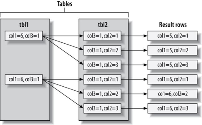
Figure 6-2. Swim-lane diagram illustrating retrieving rows using a join
MySQL executes every kind of query in essentially the same way. For example, it handles a subquery in the FROM clause by executing it first, putting the results into a temporary table,[79] and then treating that table just like an ordinary table (hence the name “derived table”). MySQL executesUNION queries with temporary tables too, and it rewrites all RIGHT OUTER JOIN queries to equivalent LEFT OUTER JOINs. In short, current versions of MySQL coerce every kind of query into this execution plan.[80]
It’s not possible to execute every legal SQL query this way, however. For example, a FULL OUTER JOIN can’t be executed with nested loops and backtracking as soon as a table with no matching rows is found, because it might begin with a table that has no matching rows. This explains why MySQL doesn’t support FULL OUTER JOIN. Still other queries can be executed with nested loops, but perform very badly as a result. We’ll look at some of those later.
The execution plan
MySQL doesn’t generate byte-code to execute a query, as many other database products do. Instead, the query execution plan is actually a tree of instructions that the query execution engine follows to produce the query results. The final plan contains enough information to reconstruct the original query. If you execute EXPLAIN EXTENDED on a query, followed by SHOW WARNINGS, you’ll see the reconstructed query.[81]
Any multitable query can conceptually be represented as a tree. For example, it might be possible to execute a four-table join as shown in Figure 6-3.
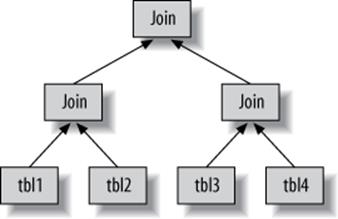
Figure 6-3. One way to join multiple tables
This is what computer scientists call a balanced tree. This is not how MySQL executes the query, though. As we described in the previous section, MySQL always begins with one table and finds matching rows in the next table. Thus, MySQL’s query execution plans always take the form of aleft-deep tree, as in Figure 6-4.
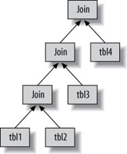
Figure 6-4. How MySQL joins multiple tables
The join optimizer
The most important part of the MySQL query optimizer is the join optimizer, which decides the best order of execution for multitable queries. It is often possible to join the tables in several different orders and get the same results. The join optimizer estimates the cost for various plans and tries to choose the least expensive one that gives the same result.
Here’s a query whose tables can be joined in different orders without changing the results:
mysql> SELECT film.film_id, film.title, film.release_year, actor.actor_id,
-> actor.first_name, actor.last_name
-> FROM sakila.film
-> INNER JOIN sakila.film_actor USING(film_id)
-> INNER JOIN sakila.actor USING(actor_id);
You can probably think of a few different query plans. For example, MySQL could begin with the film table, use the index on film_id in the film_actor table to find actor_id values, and then look up rows in the actor table’s primary key. Oracle users might phrase this as “The filmtable is the driver table into the film_actor table, which is the driver for the actor table.” This should be efficient, right? Now let’s use EXPLAIN to see how MySQL wants to execute the query:
*************************** 1. row ***************************
id: 1
select_type: SIMPLE
table: actor
type: ALL
possible_keys: PRIMARY
key: NULL
key_len: NULL
ref: NULL
rows: 200
Extra:
*************************** 2. row ***************************
id: 1
select_type: SIMPLE
table: film_actor
type: ref
possible_keys: PRIMARY,idx_fk_film_id
key: PRIMARY
key_len: 2
ref: sakila.actor.actor_id
rows: 1
Extra: Using index
*************************** 3. row ***************************
id: 1
select_type: SIMPLE
table: film
type: eq_ref
possible_keys: PRIMARY
key: PRIMARY
key_len: 2
ref: sakila.film_actor.film_id
rows: 1
Extra:
This is quite a different plan from the one suggested in the previous paragraph. MySQL wants to start with the actor table (we know this because it’s listed first in the EXPLAIN output) and go in the reverse order. Is this really more efficient? Let’s find out. The STRAIGHT_JOIN keyword forces the join to proceed in the order specified in the query. Here’s the EXPLAIN output for the revised query:
mysql> EXPLAIN SELECT STRAIGHT_JOIN film.film_id...\G
*************************** 1. row ***************************
id: 1
select_type: SIMPLE
table: film
type: ALL
possible_keys: PRIMARY
key: NULL
key_len: NULL
ref: NULL
rows: 951
Extra:
*************************** 2. row ***************************
id: 1
select_type: SIMPLE
table: film_actor
type: ref
possible_keys: PRIMARY,idx_fk_film_id
key: idx_fk_film_id
key_len: 2
ref: sakila.film.film_id
rows: 1
Extra: Using index
*************************** 3. row ***************************
id: 1
select_type: SIMPLE
table: actor
type: eq_ref
possible_keys: PRIMARY
key: PRIMARY
key_len: 2
ref: sakila.film_actor.actor_id
rows: 1
Extra:
This shows why MySQL wants to reverse the join order: doing so will enable it to examine fewer rows in the first table.[82] In both cases, it will be able to perform fast indexed lookups in the second and third tables. The difference is how many of these indexed lookups it will have to do:
§ Placing film first will require about 951 probes into film_actor and actor, one for each row in the first table.
§ If the server scans the actor table first, it will have to do only 200 index lookups into later tables.
In other words, the reversed join order will require less backtracking and rereading. To double-check the optimizer’s choice, we executed the two query versions and looked at the Last_query_cost variable for each. The reordered query had an estimated cost of 241, while the estimated cost of forcing the join order was 1,154.
This is a simple example of how MySQL’s join optimizer can reorder queries to make them less expensive to execute. Reordering joins is usually a very effective optimization. There are times when it won’t result in an optimal plan, though, and for those times you can use STRAIGHT_JOINand write the query in the order you think is best—but such times are rare. In most cases, the join optimizer will outperform a human.
The join optimizer tries to produce a query execution plan tree with the lowest achievable cost. When possible, it examines all potential combinations of subtrees, beginning with all one-table plans.
Unfortunately, a join over n tables will have n-factorial combinations of join orders to examine. This is called the search space of all possible query plans, and it grows very quickly—a 10-table join can be executed up to 3,628,800 different ways! When the search space grows too large, it can take far too long to optimize the query, so the server stops doing a full analysis. Instead, it resorts to shortcuts such as “greedy” searches when the number of tables exceeds the limit specified by the optimizer_search_depth variable (which you can change if necessary).
MySQL has many heuristics, accumulated through years of research and experimentation, that it uses to speed up the optimization stage. This can be beneficial, but it can also mean that MySQL might (on rare occasions) miss an optimal plan and choose a less optimal one because it’s trying not to examine every possible query plan.
Sometimes queries can’t be reordered, and the join optimizer can use this fact to reduce the search space by eliminating choices. A LEFT JOIN is a good example, as are correlated subqueries (more about subqueries later). This is because the results for one table depend on data retrieved from another table. These dependencies help the join optimizer reduce the search space by eliminating choices.
Sort optimizations
Sorting results can be a costly operation, so you can often improve performance by avoiding sorts or by performing them on fewer rows.
We showed you how to use indexes for sorting in Chapter 3. When MySQL can’t use an index to produce a sorted result, it must sort the rows itself. It can do this in memory or on disk, but it always calls this process a filesort, even if it doesn’t actually use a file.
If the values to be sorted will fit into the sort buffer, MySQL can perform the sort entirely in memory with a quicksort. If MySQL can’t do the sort in memory, it performs it on disk by sorting the values in chunks. It uses a quicksort to sort each chunk and then merges the sorted chunks into the results.
There are two filesort algorithms:
Two passes (old)
Reads row pointers and ORDER BY columns, sorts them, and then scans the sorted list and rereads the rows for output.
The two-pass algorithm can be quite expensive, because it reads the rows from the table twice, and the second read causes a lot of random I/O. This is especially expensive for MyISAM, which uses a system call to fetch each row (because MyISAM relies on the operating system’s cache to hold the data). On the other hand, it stores a minimal amount of data during the sort, so if the rows to be sorted are completely in memory, it can be cheaper to store less data and reread the rows to generate the final result.
Single pass (new)
Reads all the columns needed for the query, sorts them by the ORDER BY columns, and then scans the sorted list and outputs the specified columns.
This algorithm is available only in MySQL 4.1 and newer. It can be much more efficient, especially on large I/O-bound datasets, because it avoids reading the rows from the table twice and trades random I/O for more sequential I/O. However, it has the potential to use a lot more space, because it holds all the desired columns from each row, not just the columns needed to sort the rows. This means fewer tuples will fit into the sort buffer, and the filesort will have to perform more sort merge passes.
It’s tricky to say which algorithm is more efficient, and there are best and worst cases for each algorithm. MySQL uses the new algorithm if the total size of all the columns needed for the query, plus the ORDER BY columns, is no more than max_length_for_sort_data bytes, so you can use this setting to influence which algorithm is used. See Optimizing for Filesorts in Chapter 8 for more on this topic.
MySQL might use much more temporary storage space for a filesort than you’d expect, because it allocates a fixed-size record for each tuple it will sort. These records are large enough to hold the largest possible tuple, including the full length of each VARCHAR column. Also, if you’re using UTF-8, MySQL allocates three bytes for each character. As a result, we’ve seen cases where poorly optimized schemas caused the temporary space used for sorting to be many times larger than the entire table’s size on disk.
When sorting a join, MySQL might perform the filesort at two stages during the query execution. If the ORDER BY clause refers only to columns from the first table in the join order, MySQL can filesort this table and then proceed with the join. If this happens, EXPLAIN shows “Using filesort” in the Extra column. In all other circumstances—such as a sort against a table that’s not first in the join order, or when the ORDER BY clause contains columns from more than one table—MySQL must store the query’s results into a temporary table and then filesort the temporary table after the join finishes. In this case, EXPLAIN shows “Using temporary; Using filesort” in the Extra column. If there’s a LIMIT, it is applied after the filesort, so the temporary table and the filesort can be very large.
MySQL 5.6 introduces significant changes to how sorts are performed when only a subset of the rows will be needed, such as a LIMIT query. Instead of sorting the entire result set and then returning a portion of it, MySQL 5.6 can sometimes discard unwanted rows before sorting them.
The Query Execution Engine
The parsing and optimizing stage outputs a query execution plan, which MySQL’s query execution engine uses to process the query. The plan is a data structure; it is not executable byte-code, which is how many other databases execute queries.
In contrast to the optimization stage, the execution stage is usually not all that complex: MySQL simply follows the instructions given in the query execution plan. Many of the operations in the plan invoke methods implemented by the storage engine interface, also known as the handler API. Each table in the query is represented by an instance of a handler. If a table appears three times in the query, for example, the server creates three handler instances. Though we glossed over this before, MySQL actually creates the handler instances early in the optimization stage. The optimizer uses them to get information about the tables, such as their column names and index statistics.
The storage engine interface has lots of functionality, but it needs only a dozen or so “building-block” operations to execute most queries. For example, there’s an operation to read the first row in an index, and one to read the next row in an index. This is enough for a query that does an index scan. This simplistic execution method makes MySQL’s storage engine architecture possible, but it also imposes some of the optimizer limitations we’ve discussed.
NOTE
Not everything is a handler operation. For example, the server manages table locks. The handler might implement its own lower-level locking, as InnoDB does with row-level locks, but this does not replace the server’s own locking implementation. As explained in Chapter 1, anything that all storage engines share is implemented in the server, such as date and time functions, views, and triggers.
To execute the query, the server just repeats the instructions until there are no more rows to examine.
Returning Results to the Client
The final step in executing a query is to reply to the client. Even queries that don’t return a result set still reply to the client connection with information about the query, such as how many rows it affected.
If the query is cacheable, MySQL will also place the results into the query cache at this stage.
The server generates and sends results incrementally. Think back to the single-sweep multijoin method we mentioned earlier. As soon as MySQL processes the last table and generates one row successfully, it can and should send that row to the client.
This has two benefits: it lets the server avoid holding the row in memory, and it means the client starts getting the results as soon as possible.[83]
Each row in the result set is sent in a separate packet in the MySQL client/server protocol, although protocol packets can be buffered and sent together at the TCP protocol layer.
[73] If the query is too large, the server will refuse to receive any more data and throw an error.
[74] You can work around this with SQL_BUFFER_RESULT, which we’ll see a bit later.
[75] Percona Server has a feature that strips comments from queries before the hash lookup is performed, which can help make the query cache more effective when queries differ only in the text contained in their comments.
[76] For example, the range check query plan reevaluates indexes for each row in a JOIN. You can see this query plan by looking for “range checked for each record” in the Extra column in EXPLAIN. This query plan also increments the Select_full_range_join server variable.
[77] We agree, a movie without actors is strange, but the Sakila sample database lists no actors for SLACKER LIAISONS, which it describes as “A Fast-Paced Tale of a Shark And a Student who must Meet a Crocodile in Ancient China.”
[78] As we show later, MySQL’s query execution isn’t quite this simple; there are many optimizations that complicate it.
[79] There are no indexes on the temporary table, which is something you should keep in mind when writing complex joins against subqueries in the FROM clause. This applies to UNION queries, too.
[80] There are significant changes in MySQL 5.6 and in MariaDB, which introduce more sophisticated execution paths.
[81] The server generates the output from the execution plan. It thus has the same semantics as the original query, but not necessarily the same text.
[82] Strictly speaking, MySQL doesn’t try to reduce the number of rows it reads. Instead, it tries to optimize for fewer page reads. But a row count can often give you a rough idea of the query cost.
[83] You can influence this behavior if needed—for example, with the SQL_BUFFER_RESULT hint. See Query Optimizer Hints.
Limitations of the MySQL Query Optimizer
MySQL’s “everything is a nested-loop join” approach to query execution isn’t ideal for optimizing every kind of query. Fortunately, there are only a limited number of cases where the MySQL query optimizer does a poor job, and it’s usually possible to rewrite such queries more efficiently. Even better, when MySQL 5.6 is released it will eliminate many of MySQL’s limitations and make a variety of queries execute much more quickly.
Correlated Subqueries
MySQL sometimes optimizes subqueries very badly. The worst offenders are IN() subqueries in the WHERE clause. As an example, let’s find all films in the Sakila sample database’s sakila.film table whose casts include the actress Penelope Guiness (actor_id=1). This feels natural to write with a subquery, as follows:
mysql> SELECT * FROM sakila.film
-> WHERE film_id IN(
-> SELECT film_id FROM sakila.film_actor WHERE actor_id = 1);
It’s tempting to think that MySQL will execute this query from the inside out, by finding a list of actor_id values and substituting them into the IN() list. We said an IN() list is generally very fast, so you might expect the query to be optimized to something like this:
-- SELECT GROUP_CONCAT(film_id) FROM sakila.film_actor WHERE actor_id = 1;
-- Result: 1,23,25,106,140,166,277,361,438,499,506,509,605,635,749,832,939,970,980
SELECT * FROM sakila.film
WHERE film_id
IN(1,23,25,106,140,166,277,361,438,499,506,509,605,635,749,832,939,970,980);
Unfortunately, exactly the opposite happens. MySQL tries to “help” the subquery by pushing a correlation into it from the outer table, which it thinks will let the subquery find rows more efficiently. It rewrites the query as follows:
SELECT * FROM sakila.film
WHERE EXISTS (
SELECT * FROM sakila.film_actor WHERE actor_id = 1
AND film_actor.film_id = film.film_id);
Now the subquery requires the film_id from the outer film table and can’t be executed first. EXPLAIN shows the result as DEPENDENT SUBQUERY (you can use EXPLAIN EXTENDED to see exactly how the query is rewritten):
mysql> EXPLAIN SELECT * FROM sakila.film ...;
+----+--------------------+------------+--------+------------------------+
| id | select_type | table | type | possible_keys |
+----+--------------------+------------+--------+------------------------+
| 1 | PRIMARY | film | ALL | NULL |
| 2 | DEPENDENT SUBQUERY | film_actor | eq_ref | PRIMARY,idx_fk_film_id |
+----+--------------------+------------+--------+------------------------+
According to the EXPLAIN output, MySQL will table-scan the film table and execute the subquery for each row it finds. This won’t cause a noticeable performance hit on small tables, but if the outer table is very large, the performance will be extremely bad. Fortunately, it’s easy to rewrite such a query as a JOIN:
mysql> SELECT film.* FROM sakila.film
-> INNER JOIN sakila.film_actor USING(film_id)
-> WHERE actor_id = 1;
Another good optimization is to manually generate the IN() list by executing the subquery as a separate query with GROUP_CONCAT(). Sometimes this can be faster than a JOIN. And finally, although IN() subqueries work poorly in many cases, EXISTS() or equality subqueries sometimes work much better. Here is another way to rewrite our IN() subquery example:
mysql> SELECT * FROM sakila.film
-> WHERE EXISTS(
-> SELECT * FROM sakila.film_actor WHERE actor_id = 1
-> AND film_actor.film_id = film.film_id);
NOTE
The optimizer limitations we’ll discuss throughout this section apply to the official MySQL server from Oracle Corporation as of version 5.5. The MariaDB fork of MySQL has several related query optimizer and execution engine enhancements, such as executing correlated subqueries from the inside out.
When a correlated subquery is good
MySQL doesn’t always optimize correlated subqueries badly. If you hear advice to always avoid them, don’t listen! Instead, measure and make your own decision. Sometimes a correlated subquery is a perfectly reasonable, or even optimal, way to get a result. Let’s look at an example:
mysql> EXPLAIN SELECT film_id, language_id FROM sakila.film
-> WHERE NOT EXISTS(
-> SELECT * FROM sakila.film_actor
-> WHERE film_actor.film_id = film.film_id
-> )\G
*************************** 1. row ***************************
id: 1
select_type: PRIMARY
table: film
type: ALL
possible_keys: NULL
key: NULL
key_len: NULL
ref: NULL
rows: 951
Extra: Using where
*************************** 2. row ***************************
id: 2
select_type: DEPENDENT SUBQUERY
table: film_actor
type: ref
possible_keys: idx_fk_film_id
key: idx_fk_film_id
key_len: 2
ref: film.film_id
rows: 2
Extra: Using where; Using index
The standard advice for this query is to write it as a LEFT OUTER JOIN instead of using a subquery. In theory, MySQL’s execution plan will be essentially the same either way. Let’s see:
mysql> EXPLAIN SELECT film.film_id, film.language_id
-> FROM sakila.film
-> LEFT OUTER JOIN sakila.film_actor USING(film_id)
-> WHERE film_actor.film_id IS NULL\G
*************************** 1. row ***************************
id: 1
select_type: SIMPLE
table: film
type: ALL
possible_keys: NULL
key: NULL
key_len: NULL
ref: NULL
rows: 951
Extra:
*************************** 2. row ***************************
id: 1
select_type: SIMPLE
table: film_actor
type: ref
possible_keys: idx_fk_film_id
key: idx_fk_film_id
key_len: 2
ref: sakila.film.film_id
rows: 2
Extra: Using where; Using index; Not exists
The plans are nearly identical, but there are some differences:
§ The SELECT type against film_actor is DEPENDENT SUBQUERY in one query and SIMPLE in the other. This difference simply reflects the syntax, because the first query uses a subquery and the second doesn’t. It doesn’t make much difference in terms of handler operations.
§ The second query doesn’t say “Using where” in the Extra column for the film table. That doesn’t matter, though: the second query’s USING clause is the same thing as a WHERE clause anyway.
§ The second query says “Not exists” in the film_actor table’s Extra column. This is an example of the early-termination algorithm we mentioned earlier in this chapter. It means MySQL is using a not-exists optimization to avoid reading more than one row in the film_actor table’sidx_fk_film_id index. This is equivalent to a NOT EXISTS() correlated subquery, because it stops processing the current row as soon as it finds a match.
So, in theory, MySQL will execute the queries almost identically. In reality, measuring is the only way to tell which approach is really faster. We benchmarked both queries on our standard setup. The results are shown in Table 6-1.
Table 6-1. NOT EXISTS versus LEFT OUTER JOIN
|
Query |
Result in queries per second (QPS) |
|
NOT EXISTS subquery |
360 QPS |
|
LEFT OUTER JOIN |
425 QPS |
Our benchmark found that the subquery is quite a bit slower!
However, this isn’t always the case. Sometimes a subquery can be faster. For example, it can work well when you just want to see rows from one table that match rows in another table. Although that sounds like it describes a join perfectly, it’s not always the same thing. The following join, which is designed to find every film that has an actor, will return duplicates because some films have multiple actors:
mysql> SELECT film.film_id FROM sakila.film
-> INNER JOIN sakila.film_actor USING(film_id);
We need to use DISTINCT or GROUP BY to eliminate the duplicates:
mysql> SELECT DISTINCT film.film_id FROM sakila.film
-> INNER JOIN sakila.film_actor USING(film_id);
But what are we really trying to express with this query, and is it obvious from the SQL? The EXISTS operator expresses the logical concept of “has a match” without producing duplicated rows and avoids a GROUP BY or DISTINCT operation, which might require a temporary table. Here’s the query written as a subquery instead of a join:
mysql> SELECT film_id FROM sakila.film
-> WHERE EXISTS(SELECT * FROM sakila.film_actor
-> WHERE film.film_id = film_actor.film_id);
Again, we benchmarked to see which strategy was faster. The results are shown in Table 6-2.
Table 6-2. EXISTS versus INNER JOIN
|
Query |
Result in queries per second (QPS) |
|
INNER JOIN |
185 QPS |
|
EXISTS subquery |
325 QPS |
In this example, the subquery performs much faster than the join.
We showed this lengthy example to illustrate two points: you should not heed categorical advice about subqueries, and you should measure to prove your assumptions about query plans and response time. A final note on subqueries: this is one of the rare cases where we need to mention a bug in MySQL. In MySQL version 5.1.48 and earlier, the following syntax can lock a row in table2:
SELECT ... FROM table1 WHERE col = (SELECT ... FROM table2 WHERE ...);
This bug, if it affects you, can cause subqueries to behave much differently under high concurrency than if you measure their performance in a single thread. This is bug 46947, and even though it’s solved, it still reinforces our point: don’t assume.
UNION Limitations
MySQL sometimes can’t “push down” conditions from the outside of a UNION to the inside, where they could be used to limit results or enable additional optimizations.
If you think any of the individual queries inside a UNION would benefit from a LIMIT, or if you know they’ll be subject to an ORDER BY clause once combined with other queries, you need to put those clauses inside each part of the UNION. For example, if you UNION together two tables andLIMIT the result to the first 20 rows, MySQL will store both tables into a temporary table and then retrieve just 20 rows from it:
(SELECT first_name, last_name
FROM sakila.actor
ORDER BY last_name)
UNION ALL
(SELECT first_name, last_name
FROM sakila.customer
ORDER BY last_name)
LIMIT 20;
This query will store 200 rows from the actor table, and 599 from the customer table, into a temporary table and then fetch the first 20 rows from that temporary table. You can avoid this by adding LIMIT 20 redundantly to each query inside the UNION:
(SELECT first_name, last_name
FROM sakila.actor
ORDER BY last_name
LIMIT 20)
UNION ALL
(SELECT first_name, last_name
FROM sakila.customer
ORDER BY last_name
LIMIT 20)
LIMIT 20;
Now the temporary table will contain only 40 rows. In addition to the performance improvement, you’ll probably need to correct the query: the order in which the rows are retrieved from the temporary table is undefined, so there should be an overall ORDER BY just before the final LIMIT.
Index Merge Optimizations
As discussed in the previous chapter, MySQL 5.0 and greater can access several indexes from a single table and union or intersect the results to locate rows when there are complex filtering conditions in the WHERE clause.
Equality Propagation
Equality propagation can have unexpected costs sometimes. For example, consider a huge IN() list on a column the optimizer knows will be equal to some columns on other tables, due to a WHERE, ON, or USING clause that sets the columns equal to each other.
The optimizer will “share” the list by copying it to the corresponding columns in all related tables. This is normally helpful, because it gives the query optimizer and execution engine more options for where to actually execute the IN() check. But when the list is very large, it can result in slower optimization and execution. There’s no built-in workaround for this problem at the time of this writing—you’ll have to change the source code if it’s a problem for you. (It’s not a problem for most people.)
Parallel Execution
MySQL can’t execute a single query in parallel on many CPUs. This is a feature offered by some other database servers, but not MySQL. We mention it so that you won’t spend a lot of time trying to figure out how to get parallel query execution on MySQL!
Hash Joins
MySQL can’t do true hash joins at the time of this writing—everything is a nested-loop join. However, you can emulate hash joins using hash indexes. If you aren’t using the Memory storage engine, you’ll have to emulate the hash indexes, too. We showed you how to do this in Building your own hash indexes. MariaDB can perform true hash joins.
Loose Index Scans
MySQL has historically been unable to do loose index scans, which scan noncontiguous ranges of an index. MySQL’s index scans generally require a defined start point and a defined end point in the index, even if only a few noncontiguous rows in the middle are really desired for the query. MySQL will scan the entire range of rows within these end points.
An example will help clarify this. Suppose we have a table with an index on columns (a, b), and we want to run the following query:
mysql> SELECT ... FROM tbl WHERE b BETWEEN 2 AND 3;
Because the index begins with column a, but the query’s WHERE clause doesn’t specify column a, MySQL will do a table scan and eliminate the nonmatching rows with a WHERE clause, as shown in Figure 6-5.
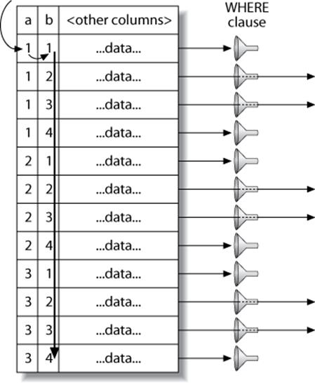
Figure 6-5. MySQL scans the entire table to find rows
It’s easy to see that there’s a faster way to execute this query. The index’s structure (but not MySQL’s storage engine API) lets you seek to the beginning of each range of values, scan until the end of the range, and then backtrack and jump ahead to the start of the next range. Figure 6-6 shows what that strategy would look like if MySQL were able to do it.
Notice the absence of a WHERE clause, which isn’t needed because the index alone lets us skip over the unwanted rows.
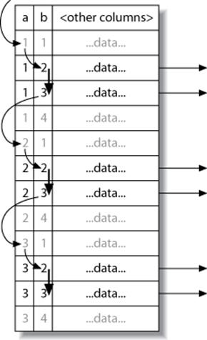
Figure 6-6. A loose index scan, which MySQL cannot currently do, would be more efficient
This is admittedly a simplistic example, and we could easily optimize the query we’ve shown by adding a different index. However, there are many cases where adding another index can’t solve the problem. One example is a query that has a range condition on the index’s first column and an equality condition on the second column.
Beginning in MySQL 5.0, loose index scans are possible in certain limited circumstances, such as queries that find maximum and minimum values in a grouped query:
mysql> EXPLAIN SELECT actor_id, MAX(film_id)
-> FROM sakila.film_actor
-> GROUP BY actor_id\G
*************************** 1. row ***************************
id: 1
select_type: SIMPLE
table: film_actor
type: range
possible_keys: NULL
key: PRIMARY
key_len: 2
ref: NULL
rows: 396
Extra: Using index for group-by
The “Using index for group-by” information in this EXPLAIN plan indicates a loose index scan. This is a good optimization for this special purpose, but it is not a general-purpose loose index scan. It might be better termed a “loose index probe.”
Until MySQL supports general-purpose loose index scans, the workaround is to supply a constant or list of constants for the leading columns of the index. We showed several examples of how to get good performance with these types of queries in our indexing case study in the previous chapter.
In MySQL 5.6, some limitations on loose index scans will be fixed with an optimizer technique called “index condition pushdown.”
MIN() and MAX()
MySQL doesn’t optimize certain MIN() and MAX() queries very well. Here’s an example:
mysql> SELECT MIN(actor_id) FROM sakila.actor WHERE first_name = 'PENELOPE';
Because there’s no index on first_name, this query performs a table scan. If MySQL scans the primary key, it can theoretically stop after reading the first matching row, because the primary key is strictly ascending and any subsequent row will have a greater actor_id. However, in this case MySQL will scan the whole table, which you can verify by looking at SHOW STATUS counters. The workaround is to remove the MIN() and rewrite the query with a LIMIT, as follows:
mysql> SELECT actor_id FROM sakila.actor USE INDEX(PRIMARY)
-> WHERE first_name = 'PENELOPE' LIMIT 1;
This general strategy often works well when MySQL would otherwise choose to scan more rows than necessary. If you’re a purist, you might object that this query is missing the point of SQL. We’re supposed to be able to tell the server what we want and it’s supposed to figure out how to get that data, whereas in this case we’re telling MySQL how to execute the query and, as a result, it’s not clear from the query that what we’re looking for is a minimal value. True, but sometimes you have to compromise your principles to get high performance.
SELECT and UPDATE on the Same Table
MySQL doesn’t let you SELECT from a table while simultaneously running an UPDATE on it. This isn’t really an optimizer limitation, but knowing how MySQL executes queries can help you work around it. Here’s an example of a query that’s disallowed, even though it is standard SQL. The query updates each row with the number of similar rows in the table:
mysql> UPDATE tbl AS outer_tbl
-> SET cnt = (
-> SELECT count(*) FROM tbl AS inner_tbl
-> WHERE inner_tbl.type = outer_tbl.type
-> );
ERROR 1093 (HY000): You can’t specify target table 'outer_tbl' for update in FROM
clause
To work around this limitation, you can use a derived table, because MySQL materializes it as a temporary table. This effectively executes two queries: one SELECT inside the subquery, and one multitable UPDATE with the joined results of the table and the subquery. The subquery opens and closes the table before the outer UPDATE opens the table, so the query will now succeed:
mysql> UPDATE tbl
-> INNER JOIN(
-> SELECT type, count(*) AS cnt
-> FROM tbl
-> GROUP BY type
-> ) AS der USING(type)
-> SET tbl.cnt = der.cnt;
Query Optimizer Hints
MySQL has a few optimizer hints you can use to control the query plan if you’re not happy with the one MySQL’s optimizer chooses. The following list identifies these hints and indicates when it’s a good idea to use them. You place the appropriate hint in the query whose plan you want to modify, and it is effective for only that query. Check the MySQL manual for the exact syntax of each hint. Some of them are version-dependent. The options are:
HIGH_PRIORITY and LOW_PRIORITY
These hints tell MySQL how to prioritize the statement relative to other statements that are trying to access the same tables.
HIGH_PRIORITY tells MySQL to schedule a SELECT statement before other statements that might be waiting for table locks so they can modify data. In effect, it makes the SELECT go to the front of the queue instead of waiting its turn. You can also apply this modifier to INSERT, where it simply cancels the effect of a global LOW_PRIORITY server setting.
LOW_PRIORITY is the reverse: it makes the statement wait at the very end of the queue if there are any other statements that want to access the tables—even if the other statements are issued after it. It’s rather like an overly polite person holding the door at a restaurant: as long as there’s anyone else waiting, it will starve itself! You can apply this hint to SELECT, INSERT, UPDATE, REPLACE, and DELETE statements.
These hints are effective on storage engines with table-level locking, but you should never need them on InnoDB or other engines with fine-grained locking and concurrency control. Be careful when using them on MyISAM, because they can disable concurrent inserts and greatly reduce performance.
The HIGH_PRIORITY and LOW_PRIORITY hints are a frequent source of confusion. They do not allocate more or fewer resources to queries to make them “work harder” or “not work as hard”; they simply affect how the server queues statements that are waiting for access to a table.
DELAYED
This hint is for use with INSERT and REPLACE. It lets the statement to which it is applied return immediately and places the inserted rows into a buffer, which will be inserted in bulk when the table is free. This is most useful for logging and similar applications where you want to insert a lot of rows without making the client wait, and without causing I/O for each statement. There are many limitations; for example, delayed inserts are not implemented in all storage engines, and LAST_INSERT_ID() doesn’t work with them.
STRAIGHT_JOIN
This hint can appear either just after the SELECT keyword in a SELECT statement, or in any statement between two joined tables. The first usage forces all tables in the query to be joined in the order in which they’re listed in the statement. The second usage forces a join order on the two tables between which the hint appears.
The STRAIGHT_JOIN hint is useful when MySQL doesn’t choose a good join order, or when the optimizer takes a long time to decide on a join order. In the latter case, the thread will spend a lot of time in the “statistics” state, and adding this hint will reduce the search space for the optimizer.
You can use EXPLAIN to see what order the optimizer would choose, then rewrite the query in that order and add STRAIGHT_JOIN. This is a good idea as long as you don’t think the fixed order will result in bad performance for some WHERE clauses. You should be careful to revisit such queries after upgrading MySQL, however, because new optimizations might appear that will be defeated by STRAIGHT_JOIN.
SQL_SMALL_RESULT and SQL_BIG_RESULT
These hints are for SELECT statements. They tell the optimizer how and when to use temporary tables and sort in GROUP BY or DISTINCT queries. SQL_SMALL_RESULT tells the optimizer that the result set will be small and can be put into indexed temporary tables to avoid sorting for the grouping, whereas SQL_BIG_RESULT indicates that the result will be large and that it will be better to use temporary tables on disk with sorting.
SQL_BUFFER_RESULT
This hint tells the optimizer to put the results into a temporary table and release table locks as soon as possible. This is different from the client-side buffering we described previously. Server-side buffering can be useful when you don’t use buffering on the client, because it lets you avoid consuming a lot of memory on the client and still release locks quickly. The trade-off is that the server’s memory is used instead of the client’s.
SQL_CACHE and SQL_NO_CACHE
These hints instruct the server that the query either is or is not a candidate for caching in the query cache. See the next chapter for details on how to use them.
SQL_CALC_FOUND_ROWS
This hint isn’t strictly an optimizer hint. It doesn’t tell MySQL to plan the query differently. Instead, it provides extra functionality by changing what the query actually does. It tells MySQL to calculate a full result set when there’s a LIMIT clause, even though it returns only LIMIT rows. You can retrieve the total number of rows it found via FOUND_ROWS() (but take a look at the section Optimizing SQL_CALC_FOUND_ROWS for reasons why you shouldn’t use this hint).
FOR UPDATE and LOCK IN SHARE MODE
These hints aren’t really optimizer hints, either; they control locking for SELECT statements, but only for storage engines that have row-level locks. They enable you to place locks on the matched rows. These hints are not needed for INSERT ... SELECT queries, which place read locks on the source rows by default in MySQL 5.0 and newer versions. (You can disable this behavior, but it’s not a good idea—we explain why in the chapters on replication and backups.)
The only built-in storage engine that supports these hints is InnoDB. Be aware that they disable some optimizations, such as covering indexes. InnoDB can’t lock rows exclusively without accessing the primary key, which is where the row versioning information is stored.
Unfortunately, these hints are way overused and frequently cause severe locking problems, as we’ll discuss later in this chapter. You should avoid them at pretty much all costs; there’s usually a better way to do what you’re trying to do.
USE INDEX, IGNORE INDEX, and FORCE INDEX
These hints tell the optimizer which indexes to use or ignore for finding rows in a table (for example, when deciding on a join order). In MySQL 5.0 and earlier, they don’t influence which indexes the server uses for sorting and grouping; in MySQL 5.1 the syntax can take an optional FOR ORDER BY or FOR GROUP BY clause.
FORCE INDEX is the same as USE INDEX, but it tells the optimizer that a table scan is extremely expensive compared to the index, even if the index is not very useful. You can use these hints when you don’t think the optimizer is choosing the right index, or when you want to take advantage of an index for some reason, such as implicit ordering without an ORDER BY. We gave an example of this previously, where we showed how to get a minimum value efficiently with LIMIT.
In MySQL 5.0 and newer, there are also some configuration variables that influence the optimizer:
optimizer_search_depth
This variable tells the optimizer how exhaustively to examine partial plans. If your queries are taking a very long time in the “Statistics” state, you might try lowering this value.
optimizer_prune_level
This variable, which is enabled by default, lets the optimizer skip certain plans based on the number of rows examined.
optimizer_switch
This variable contains a set of flags that enable or disable specific optimizer features. For example, in MySQL 5.1 you can use it to disable the index merge query plan.
The first two options control optimizer shortcuts. These shortcuts are valuable for good performance on complex queries, but they can cause the server to miss optimal plans for the sake of efficiency. That’s why it sometimes makes sense to change them.
VALIDATING MYSQL UPGRADES
Trying to outsmart the MySQL optimizer usually is not a good idea. It generally creates more work and increases maintenance costs for very little benefit. This is especially relevant when you upgrade MySQL, because optimizer hints used in your queries might prevent new optimizer strategies from being used.
In MySQL 5.0 a number of capabilities were added to the optimizer, and the as-yet unreleased MySQL 5.6 will have the biggest changes to the optimizer in a very long time. If you are upgrading to one of these versions, you will not want to miss out on the benefits they offer.
New versions of MySQL generally improve the server by leaps and bounds, and this is especially true in the 5.5 and 5.6 versions. MySQL upgrades usually go fine, but you still need to test changes carefully. There is always a chance that you will discover an edge case that affects you. The good news is that it’s really easy to prevent this with a little change management. Use the pt-upgradetool from Percona Toolkit to validate that your queries run well on the new version of MySQL, and that they don’t return different results.
Optimizing Specific Types of Queries
In this section, we give advice on how to optimize certain kinds of queries. We’ve covered most of these topics in detail elsewhere in the book, but we wanted to make a list of common optimization problems that you can refer to easily.
Most of the advice in this section is version-dependent, and it might not hold for future versions of MySQL. There’s no reason why the server won’t be able to do some or all of these optimizations itself someday.
Optimizing COUNT() Queries
The COUNT() aggregate function, and how to optimize queries that use it, is probably one of the top 10 most-misunderstood topics in MySQL. You can do a web search and find more misinformation on this topic than we care to think about.
Before we get into optimization, it’s important that you understand what COUNT() really does.
What COUNT() does
COUNT() is a special function that works in two very different ways: it counts values and rows. A value is a non-NULL expression (NULL is the absence of a value). If you specify a column name or other expression inside the parentheses, COUNT() counts how many times that expression has a value. This is confusing for many people, in part because values and NULL are confusing. If you need to learn how this works in SQL, we suggest a good book on SQL fundamentals. (The Internet is not necessarily a good source of accurate information on this topic.)
The other form of COUNT() simply counts the number of rows in the result. This is what MySQL does when it knows the expression inside the parentheses can never be NULL. The most obvious example is COUNT(*), which is a special form of COUNT() that does not expand the * wildcard into the full list of columns in the table, as you might expect; instead, it ignores columns altogether and counts rows.
One of the most common mistakes we see is specifying column names inside the parentheses when you want to count rows. When you want to know the number of rows in the result, you should always use COUNT(*). This communicates your intention clearly and avoids poor performance.
Myths about MyISAM
A common misconception is that MyISAM is extremely fast for COUNT() queries. It is fast, but only for a very special case: COUNT(*) without a WHERE clause, which merely counts the number of rows in the entire table. MySQL can optimize this away because the storage engine always knows how many rows are in the table. If MySQL knows col can never be NULL, it can also optimize a COUNT(col) expression by converting it to COUNT(*) internally.
MyISAM does not have any magical speed optimizations for counting rows when the query has a WHERE clause, or for the more general case of counting values instead of rows. It might be faster than other storage engines for a given query, or it might not be. That depends on a lot of factors.
Simple optimizations
You can sometimes use MyISAM’s COUNT(*) optimization to your advantage when you want to count all but a very small number of rows that are well indexed. The following example uses the standard world database to show how you can efficiently find the number of cities whose ID is greater than 5. You might write this query as follows:
mysql> SELECT COUNT(*) FROM world.City WHERE ID > 5;
If you examine this query with SHOW STATUS, you’ll see that it scans 4,079 rows. If you negate the conditions and subtract the number of cities whose IDs are less than or equal to 5 from the total number of cities, you can reduce that to five rows:
mysql> SELECT (SELECT COUNT(*) FROM world.City) - COUNT(*)
-> FROM world.City WHERE ID <= 5;
This version reads fewer rows because the subquery is turned into a constant during the query optimization phase, as you can see with EXPLAIN:
+----+-------------+-------+...+------+------------------------------+
| id | select_type | table |...| rows | Extra |
+----+-------------+-------+...+------+------------------------------+
| 1 | PRIMARY | City |...| 6 | Using where; Using index |
| 2 | SUBQUERY | NULL |...| NULL | Select tables optimized away |
+----+-------------+-------+...+------+------------------------------+
A frequent question on mailing lists and IRC channels is how to retrieve counts for several different values in the same column with just one query, to reduce the number of queries required. For example, say you want to create a single query that counts how many items have each of several colors. You can’t use an OR (e.g., SELECT COUNT(color = 'blue' OR color = 'red') FROM items;), because that won’t separate the different counts for the different colors. And you can’t put the colors in the WHERE clause (e.g., SELECT COUNT(*) FROM items WHERE color = 'blue' AND color = 'red';), because the colors are mutually exclusive. Here is a query that solves this problem:[84]
mysql> SELECT SUM(IF(color = 'blue', 1, 0)) AS blue,SUM(IF(color = 'red', 1, 0))
-> AS red FROM items;
And here is another that’s equivalent, but instead of using SUM() uses COUNT() and ensures that the expressions won’t have values when the criteria are false:
mysql> SELECT COUNT(color = 'blue' OR NULL) AS blue, COUNT(color = 'red' OR NULL)
-> AS red FROM items;
Using an approximation
Sometimes you don’t need an accurate count, so you can just use an approximation. The optimizer’s estimated rows in EXPLAIN often serves well for this. Just execute an EXPLAIN query instead of the real query.
At other times, an exact count is much less efficient than an approximation. One customer asked for help counting the number of active users on his website. The user count was cached and displayed for 30 minutes, after which it was regenerated and cached again. This was inaccurate by nature, so an approximation was acceptable. The query included several WHERE conditions to ensure that it didn’t count inactive users or the “default” user, which was a special user ID in the application. Removing these conditions changed the count only slightly, but made the query much more efficient. A further optimization was to eliminate an unnecessary DISTINCT to remove a filesort. The rewritten query was much faster and returned almost exactly the same results.
More complex optimizations
In general, COUNT() queries are hard to optimize because they usually need to count a lot of rows (i.e., access a lot of data). Your only other option for optimizing within MySQL itself is to use a covering index. If that doesn’t help enough, you need to make changes to your application architecture. Consider summary tables (covered in Chapter 4), and possibly an external caching system such as memcached. You’ll probably find yourself faced with the familiar dilemma, “fast, accurate, and simple: pick any two.”
Optimizing JOIN Queries
This topic is actually spread throughout most of the book, but we’ll mention a few highlights:
§ Make sure there are indexes on the columns in the ON or USING clauses. Consider the join order when adding indexes. If you’re joining tables A and B on column c and the query optimizer decides to join the tables in the order B, A, you don’t need to index the column on table B. Unused indexes are extra overhead. In general, you need to add indexes only on the second table in the join order, unless they’re needed for some other reason.
§ Try to ensure that any GROUP BY or ORDER BY expression refers only to columns from a single table, so MySQL can try to use an index for that operation.
§ Be careful when upgrading MySQL, because the join syntax, operator precedence, and other behaviors have changed at various times. What used to be a normal join can sometimes become a cross product, a different kind of join that returns different results, or even invalid syntax.
Optimizing Subqueries
The most important advice we can give on subqueries is that you should usually prefer a join where possible, at least in current versions of MySQL. We covered this topic extensively earlier in this chapter. However, “prefer a join” is not future-proof advice, and if you’re using MySQL 5.6 or newer versions, or MariaDB, subqueries are a whole different matter.
Optimizing GROUP BY and DISTINCT
MySQL optimizes these two kinds of queries similarly in many cases, and in fact converts between them as needed internally during the optimization process. Both types of queries benefit from indexes, as usual, and that’s the single most important way to optimize them.
MySQL has two kinds of GROUP BY strategies when it can’t use an index: it can use a temporary table or a filesort to perform the grouping. Either one can be more efficient for any given query. You can force the optimizer to choose one method or the other with the SQL_BIG_RESULT andSQL_SMALL_RESULT optimizer hints, as discussed earlier in this chapter.
If you need to group a join by a value that comes from a lookup table, it’s usually more efficient to group by the lookup table’s identifier than by the value. For example, the following query isn’t as efficient as it could be:
mysql> SELECT actor.first_name, actor.last_name, COUNT(*)
-> FROM sakila.film_actor
-> INNER JOIN sakila.actor USING(actor_id)
-> GROUP BY actor.first_name, actor.last_name;
The query is more efficiently written as follows:
mysql> SELECT actor.first_name, actor.last_name, COUNT(*)
-> FROM sakila.film_actor
-> INNER JOIN sakila.actor USING(actor_id)
-> GROUP BY film_actor.actor_id;
Grouping by actor.actor_id could be even more efficient than grouping by film_actor.actor_id. You should test on your specific data to see.
This query takes advantage of the fact that the actor’s first and last name are dependent on the actor_id, so it will return the same results, but it’s not always the case that you can blithely select nongrouped columns and get the same result. You might even have the server’s SQL_MODEconfigured to disallow it. You can use MIN() or MAX() to work around this when you know the values within the group are distinct because they depend on the grouped-by column, or if you don’t care which value you get:
mysql> SELECT MIN(actor.first_name), MAX(actor.last_name), ...;
Purists will argue that you’re grouping by the wrong thing, and they’re right. A spurious MIN() or MAX() is a sign that the query isn’t structured correctly. However, sometimes your only concern will be making MySQL execute the query as quickly as possible. The purists will be satisfied with the following way of writing the query:
mysql> SELECT actor.first_name, actor.last_name, c.cnt
-> FROM sakila.actor
-> INNER JOIN (
-> SELECT actor_id, COUNT(*) AS cnt
-> FROM sakila.film_actor
-> GROUP BY actor_id
-> ) AS c USING(actor_id) ;
But the cost of creating and filling the temporary table required for the subquery may be high compared to the cost of fudging pure relational theory a little bit. Remember, the temporary table created by the subquery has no indexes.[85]
It’s generally a bad idea to select nongrouped columns in a grouped query, because the results will be nondeterministic and could easily change if you change an index or the optimizer decides to use a different strategy. Most such queries we see are accidents (because the server doesn’t complain), or are the result of laziness rather than being designed that way for optimization purposes. It’s better to be explicit. In fact, we suggest that you set the server’s SQL_MODE configuration variable to include ONLY_FULL_GROUP_BY so it produces an error instead of letting you write a bad query.
MySQL automatically orders grouped queries by the columns in the GROUP BY clause, unless you specify an ORDER BY clause explicitly. If you don’t care about the order and you see this causing a filesort, you can use ORDER BY NULL to skip the automatic sort. You can also add an optional DESC or ASC keyword right after the GROUP BY clause to order the results in the desired direction by the clause’s columns.
Optimizing GROUP BY WITH ROLLUP
A variation on grouped queries is to ask MySQL to do superaggregation within the results. You can do this with a WITH ROLLUP clause, but it might not be as well optimized as you need. Check the execution method with EXPLAIN, paying attention to whether the grouping is done via filesort or temporary table; try removing the WITH ROLLUP and seeing if you get the same group method. You might be able to force the grouping method with the hints we mentioned earlier in this section.
Sometimes it’s more efficient to do superaggregation in your application, even if it means fetching many more rows from the server. You can also nest a subquery in the FROM clause or use a temporary table to hold intermediate results, and then query the temporary table with a UNION.
The best approach might be to move the WITH ROLLUP functionality into your application code.
Optimizing LIMIT and OFFSET
Queries with LIMITs and OFFSETs are common in systems that do pagination, nearly always in conjunction with an ORDER BY clause. It’s helpful to have an index that supports the ordering; otherwise, the server has to do a lot of filesorts.
A frequent problem is having a high value for the offset. If your query looks like LIMIT 10000, 20, it is generating 10,020 rows and throwing away the first 10,000 of them, which is very expensive. Assuming all pages are accessed with equal frequency, such queries scan half the table on average. To optimize them, you can either limit how many pages are permitted in a pagination view, or try to make the high offsets more efficient.
One simple technique to improve efficiency is to do the offset on a covering index, rather than the full rows. You can then join the result to the full row and retrieve the additional columns you need. This can be much more efficient. Consider the following query:
mysql> SELECT film_id, description FROM sakila.film ORDER BY title LIMIT 50, 5;
If the table is very large, this query is better written as follows:
mysql> SELECT film.film_id, film.description
-> FROM sakila.film
-> INNER JOIN (
-> SELECT film_id FROM sakila.film
-> ORDER BY title LIMIT 50, 5
-> ) AS lim USING(film_id);
This “deferred join” works because it lets the server examine as little data as possible in an index without accessing rows, and then, once the desired rows are found, join them against the full table to retrieve the other columns from the row. A similar technique applies to joins with LIMITclauses.
Sometimes you can also convert the limit to a positional query, which the server can execute as an index range scan. For example, if you precalculate and index a position column, you can rewrite the query as follows:
mysql> SELECT film_id, description FROM sakila.film
-> WHERE position BETWEEN 50 AND 54 ORDER BY position;
Ranked data poses a similar problem, but usually mixes GROUP BY into the fray. You’ll almost certainly need to precompute and store ranks.
The problem with LIMIT and OFFSET is really the OFFSET, which represents rows the server is generating and throwing away. If you use a sort of bookmark to remember the position of the last row you fetched, you can generate the next set of rows by starting from that position instead of using an OFFSET. For example, if you want to paginate through rental records, starting from the newest rentals and working backward, you can rely on the fact that their primary keys are always increasing. You can fetch the first set of results like this:
mysql> SELECT * FROM sakila.rental
-> ORDER BY rental_id DESC LIMIT 20;
This query returns rentals 16049 through 16030. The next query can continue from that point:
mysql> SELECT * FROM sakila.rental
-> WHERE rental_id < 16030
-> ORDER BY rental_id DESC LIMIT 20;
The nice thing about this technique is that it’s very efficient no matter how far you paginate into the table.
Other alternatives include using precomputed summaries, or joining against redundant tables that contain only the primary key and the columns you need for the ORDER BY. You can also use Sphinx; see Appendix F for more information.
Optimizing SQL_CALC_FOUND_ROWS
Another common technique for paginated displays is to add the SQL_CALC_FOUND_ROWS hint to a query with a LIMIT, so you’ll know how many rows would have been returned without the LIMIT. It might seem that there’s some kind of “magic” happening here, whereby the server predicts how many rows it would have found. But unfortunately, the server doesn’t really do that; it can’t count rows it doesn’t actually find. This option just tells the server to generate and throw away the rest of the result set, instead of stopping when it reaches the desired number of rows. That’s very expensive.
A better design is to convert the pager to a “next” link. Assuming there are 20 results per page, the query should then use a LIMIT of 21 rows and display only 20. If the 21st row exists in the results, there’s a next page, and you can render the “next” link.
Another possibility is to fetch and cache many more rows than you need—say, 1,000—and then retrieve them from the cache for successive pages. This strategy lets your application know how large the full result set is. If it’s fewer than 1,000 rows, the application knows how many page links to render; if it’s more, the application can just display “more than 1,000 results found.” Both strategies are much more efficient than repeatedly generating an entire result and discarding most of it.
Sometimes you can also just estimate the full size of the result set by running an EXPLAIN query and looking at the rows column in the result (hey, even Google doesn’t show exact result counts!). If you can’t use these tactics, using a separate COUNT(*) query to find the number of rows can be much faster than SQL_CALC_FOUND_ROWS, if it can use a covering index.
Optimizing UNION
MySQL always executes UNION queries by creating a temporary table and filling it with the UNION results. MySQL can’t apply as many optimizations to UNION queries as you might be used to. You might have to help the optimizer by manually “pushing down” WHERE, LIMIT, ORDER BY, and other conditions (i.e., copying them, as appropriate, from the outer query into each SELECT in the UNION).
It’s important to always use UNION ALL, unless you need the server to eliminate duplicate rows. If you omit the ALL keyword, MySQL adds the distinct option to the temporary table, which uses the full row to determine uniqueness. This is quite expensive. Be aware that the ALL keyword doesn’t eliminate the temporary table, though. MySQL always places results into a temporary table and then reads them out again, even when it’s not really necessary (for example, when the results could be returned directly to the client).
Static Query Analysis
Percona Toolkit contains pt-query-advisor, a tool that parses a log of queries, analyzes the query patterns, and gives annoyingly detailed advice about potentially bad practices in them. It’s sort of a “lint checker” for MySQL queries. It will catch many common problems such as those we’ve mentioned in the previous sections.
Using User-Defined Variables
It’s easy to forget about MySQL’s user-defined variables, but they can be a powerful technique for writing efficient queries. They work especially well for queries that benefit from a mixture of procedural and relational logic. Purely relational queries treat everything as unordered sets that the server somehow manipulates all at once. MySQL takes a more pragmatic approach. This can be a weakness, but it can be a strength if you know how to exploit it, and user-defined variables can help.
User-defined variables are temporary containers for values, which persist as long as your connection to the server lives. You define them by simply assigning to them with a SET or SELECT statement:[86]
mysql> SET @one := 1;
mysql> SET @min_actor := (SELECT MIN(actor_id) FROM sakila.actor);
mysql> SET @last_week := CURRENT_DATE-INTERVAL 1 WEEK;
You can then use the variables in most places an expression can go:
mysql> SELECT ... WHERE col <= @last_week;
Before we get into the strengths of user-defined variables, let’s take a look at some of their peculiarities and disadvantages and see what things you can’t use them for:
§ They disable the query cache.
§ You can’t use them where a literal or identifier is needed, such as for a table or column name, or in the LIMIT clause.
§ They are connection-specific, so you can’t use them for interconnection communication.
§ If you’re using connection pooling or persistent connections, they can cause seemingly isolated parts of your code to interact. (If so, it’s because of a bug in your code or the connection pool, but it can still happen.)
§ They are case sensitive in MySQL versions prior to 5.0, so beware of compatibility issues.
§ You can’t explicitly declare these variables’ types, and the point at which types are decided for undefined variables differs across MySQL versions. The best thing to do is initially assign a value of 0 for variables you want to use for integers, 0.0 for floating-point numbers, or '' (the empty string) for strings. A variable’s type changes when it is assigned to; MySQL’s user-defined variable typing is dynamic.
§ The optimizer might optimize away these variables in some situations, preventing them from doing what you want.
§ Order of assignment, and indeed even the time of assignment, can be nondeterministic and depend on the query plan the optimizer chose. The results can be very confusing, as you’ll see later.
§ The := assignment operator has lower precedence than any other operator, so you have to be careful to parenthesize explicitly.
§ Undefined variables do not generate a syntax error, so it’s easy to make mistakes without knowing it.
Optimizing ranking queries
One of the most important features of variables is that you can assign a value to a variable and use the resulting value at the same time. In other words, an assignment is an L-value. Here’s an example that simultaneously calculates and outputs a “row number” for a query:
mysql> SET @rownum := 0;
mysql> SELECT actor_id, @rownum := @rownum + 1 AS rownum
-> FROM sakila.actor LIMIT 3;
+----------+--------+
| actor_id | rownum |
+----------+--------+
| 1 | 1 |
| 2 | 2 |
| 3 | 3 |
+----------+--------+
This example isn’t terribly interesting, because it just shows that we can duplicate the table’s primary key. Still, it has its uses—one of which is ranking. Let’s write a query that returns the 10 actors who have played in the most movies, with a rank column that gives actors the same rank if they’re tied. We start with a query that finds the actors and the number of movies:
mysql> SELECT actor_id, COUNT(*) as cnt
-> FROM sakila.film_actor
-> GROUP BY actor_id
-> ORDER BY cnt DESC
-> LIMIT 10;
+----------+-----+
| actor_id | cnt |
+----------+-----+
| 107 | 42 |
| 102 | 41 |
| 198 | 40 |
| 181 | 39 |
| 23 | 37 |
| 81 | 36 |
| 106 | 35 |
| 60 | 35 |
| 13 | 35 |
| 158 | 35 |
+----------+-----+
Now let’s add the rank, which should be the same for all the actors who played in 35 movies. We use three variables to do this: one to keep track of the current rank, one to keep track of the previous actor’s movie count, and one to keep track of the current actor’s movie count. We change the rank when the movie count changes. Here’s a first try:
mysql> SET @curr_cnt := 0, @prev_cnt := 0, @rank := 0;
mysql> SELECT actor_id,
-> @curr_cnt := COUNT(*) AS cnt,
-> @rank := IF(@prev_cnt <> @curr_cnt, @rank + 1, @rank) AS rank,
-> @prev_cnt := @curr_cnt AS dummy
-> FROM sakila.film_actor
-> GROUP BY actor_id
-> ORDER BY cnt DESC
-> LIMIT 10;
+----------+-----+------+-------+
| actor_id | cnt | rank | dummy |
+----------+-----+------+-------+
| 107 | 42 | 0 | 0 |
| 102 | 41 | 0 | 0 |
...
Oops—the rank and count never got updated from zero. Why did this happen?
It’s impossible to give a one-size-fits-all answer. The problem could be as simple as a misspelled variable name (in this example it’s not), or something more involved. In this case, EXPLAIN shows there’s a temporary table and filesort, so the variables are being evaluated at a different time from when we expected.
This is the type of inscrutable behavior you might experience with MySQL’s user-defined variables. Debugging such problems can be tough, but it can really pay off. Ranking in SQL normally requires quadratic algorithms, such as counting the distinct number of actors who played in a greater number of movies. A user-defined variable solution can be a linear algorithm—quite an improvement.
An easy solution in this case is to add another level of temporary tables to the query, using a subquery in the FROM clause:
mysql> SET @curr_cnt := 0, @prev_cnt := 0, @rank := 0;
-> SELECT actor_id,
-> @curr_cnt := cnt AS cnt,
-> @rank := IF(@prev_cnt <> @curr_cnt, @rank + 1, @rank) AS rank,
-> @prev_cnt := @curr_cnt AS dummy
-> FROM (
-> SELECT actor_id, COUNT(*) AS cnt
-> FROM sakila.film_actor
-> GROUP BY actor_id
-> ORDER BY cnt DESC
-> LIMIT 10
-> ) as der;
+----------+-----+------+-------+
| actor_id | cnt | rank | dummy |
+----------+-----+------+-------+
| 107 | 42 | 1 | 42 |
| 102 | 41 | 2 | 41 |
| 198 | 40 | 3 | 40 |
| 181 | 39 | 4 | 39 |
| 23 | 37 | 5 | 37 |
| 81 | 36 | 6 | 36 |
| 106 | 35 | 7 | 35 |
| 60 | 35 | 7 | 35 |
| 13 | 35 | 7 | 35 |
| 158 | 35 | 7 | 35 |
+----------+-----+------+-------+
Avoiding retrieving the row just modified
What if you want to update a row, but then you want to retrieve some information about it without actually accessing the row again? Unfortunately, MySQL doesn’t support anything like PostgreSQL’s UPDATE RETURNING functionality, which would be useful for this purpose. But you can use variables instead. For example, one of our customers wanted a more efficient way to update a row’s timestamp to the current time, and then find out what that time was. The code looked like the following:
UPDATE t1 SET lastUpdated = NOW() WHERE id = 1;
SELECT lastUpdated FROM t1 WHERE id = 1;
We rewrote those queries to use a variable instead, as follows:
UPDATE t1 SET lastUpdated = NOW() WHERE id = 1 AND @now := NOW();
SELECT @now;
There are still two queries and two network round-trips, but the second query doesn’t access any tables, so it’s faster. (Your mileage may vary. This might not be worthwhile for you, but it was for this customer.)
Counting UPDATEs and INSERTs
What if you’re using INSERT ON DUPLICATE KEY UPDATE and you want to know how many rows were inserted without conflicting with existing rows, versus the rows that caused a conflict and updated a row? Kristian Köhntopp posted a solution to this problem on his blog.[87] The essence of the technique follows:
INSERT INTO t1(c1, c2) VALUES(4, 4), (2, 1), (3, 1)
ON DUPLICATE KEY UPDATE
c1 = VALUES(c1) + ( 0 * ( @x := @x +1 ) );
The query increments the @x variable when there is a conflict that causes the UPDATE portion of the query to execute. It hides the variable’s value inside an expression that is multiplied by zero, so the variable doesn’t affect the ultimate value assigned to the column. The MySQL client protocol returns the total rows affected, so there is no need to count that with a user variable.
Making evaluation order deterministic
Most problems with user variables come from assigning to them and reading them at different stages in the query. For example, it doesn’t work predictably to assign them in the SELECT statement and read from them in the WHERE clause. The following query might look like it will just return one row, but it doesn’t:
mysql> SET @rownum := 0;
mysql> SELECT actor_id, @rownum := @rownum + 1 AS cnt
-> FROM sakila.actor
-> WHERE @rownum <= 1;
+----------+------+
| actor_id | cnt |
+----------+------+
| 1 | 1 |
| 2 | 2 |
+----------+------+
This happens because the WHERE and SELECT are different stages in the query execution process. This is even more obvious when you add another stage to execution with an ORDER BY:
mysql> SET @rownum := 0;
mysql> SELECT actor_id, @rownum := @rownum + 1 AS cnt
-> FROM sakila.actor
-> WHERE @rownum <= 1
-> ORDER BY first_name;
This query returns every row in the table, because the ORDER BY added a filesort and the WHERE is evaluated before the filesort. The solution to this problem is to assign and read in the same stage of query execution:
mysql> SET @rownum := 0;
mysql> SELECT actor_id, @rownum AS rownum
-> FROM sakila.actor
-> WHERE (@rownum := @rownum + 1) <= 1;
+----------+--------+
| actor_id | rownum |
+----------+--------+
| 1 | 1 |
+----------+--------+
Pop quiz: what will happen if you add the ORDER BY back to this query? Try it and see. If you didn’t get the results you expected, why not? What about the following query, where the ORDER BY changes the variable’s value and the WHERE clause evaluates it?
mysql> SET @rownum := 0;
mysql> SELECT actor_id, first_name, @rownum AS rownum
-> FROM sakila.actor
-> WHERE @rownum <= 1
-> ORDER BY first_name, LEAST(0, @rownum := @rownum + 1);
The answer to most unexpected user-defined variable behavior can be found by running EXPLAIN and looking for “Using where,” “Using temporary,” or “Using filesort” in the Extra column.
The last example introduced another useful hack: we placed the assignment in the LEAST() function, so its value is effectively masked and won’t skew the results of the ORDER BY (as we’ve written it, the LEAST() function will always return 0). This trick is very helpful when you want to do variable assignments solely for their side effects: it lets you hide the return value and avoid extra columns, such as the dummy column we showed in a previous example. The GREATEST(), LENGTH(), ISNULL(), NULLIF(), IF(), and COALESCE() functions are also useful for this purpose, alone and in combination, because they have special behaviors. For instance, COALESCE() stops evaluating its arguments as soon as one has a defined value.
Writing a lazy UNION
Suppose you want to write a UNION query that executes the first branch of the UNION and, if it finds any rows, skips the second branch. You might do this when you’re looking for a row in a table that has “hot” rows that are accessed frequently, and another table with identical rows that happen to be accessed less often. (Partitioning hot and cold data can be a helpful way to increase cache efficiency.)
Here’s a query that will look for a user in two places—the main user table, and a table of users who haven’t visited in a long time and so have been archived for efficiency:[88]
SELECT id FROM users WHERE id = 123
UNION ALL
SELECT id FROM users_archived WHERE id = 123;
That query works, but it’ll look for the row in the users_archived table even if it is found in the users table. We can prevent that with a lazy UNION, which lazily accesses the second table only if there are no results in the first one. We’ll assign to a user variable called @found when a row is found. To make that happen, we need to place the assignment in the column list, so we’ll use the GREATEST function as a container for the assignment so we don’t get an extra column in the results. To make it easier to see which table the results came from, we’ll add a column containing the table name. Finally, we need to reset the user variable to NULL at the end of the query, so it has no side effects and can be executed repeatedly. Here’s the query:
SELECT GREATEST(@found := −1, id) AS id, 'users' AS which_tbl
FROM users WHERE id = 1
UNION ALL
SELECT id, 'users_archived'
FROM users_archived WHERE id = 1 AND @found IS NULL
UNION ALL
SELECT 1, 'reset' FROM DUAL WHERE ( @found := NULL ) IS NOT NULL;
Other uses for variables
You can put variable assignments in all types of statements, not just SELECT statements. In fact, this is one of the best uses for user-defined variables. For example, you can rewrite expensive queries, such as rank calculations with subqueries, as cheap once-through UPDATE statements.
It can be a little tricky to get the desired behavior, though. Sometimes the optimizer decides to consider the variables as compile-time constants and refuses to perform assignments. Placing the assignments inside a function like LEAST() will usually help. Another tip is to check whether your variable has a defined value before executing the containing statement. Sometimes you want it to, but other times you don’t.
With a little experimentation, you can do all sorts of interesting things with user-defined variables. Here are some ideas:
§ Calculate running totals and averages
§ Emulate FIRST() and LAST() functions for grouped queries
§ Do math on extremely large numbers
§ Reduce an entire table to a single MD5 hash value
§ “Unwrap” a sampled value that wraps around to zero when it increases beyond a certain boundary
§ Emulate read/write cursors
§ Put variables in SHOW statements by embedding them into the WHERE clause
THE C. J. DATE DILEMMA
C. J. Date advocates a database design approach that treats SQL databases as closely as possible to relational databases. It is enlightening to know how SQL deviates from the relational model, and frankly MySQL goes farther afield than some database management systems. However, you won’t get good performance from MySQL if you try to force it to behave like a relational database with some of the techniques Mr. Date advocates in his books, such as deeply nested subqueries. It’s unfortunate, but MySQL’s limitations prevent a more formal approach from working well. We recommend reading his book SQL and Relational Theory: How to Write Accurate SQL Code (O’Reilly). It’ll change the way you think about SQL.
[84] You can also write the SUM() expressions as SUM(color = 'blue'), SUM(color = 'red').
[85] This is another limitation that’s fixed in MariaDB, by the way.
[86] In some contexts you can assign with a plain = sign, but we think it’s better to avoid ambiguity and always use :=.
[87] See http://mysqldump.azundris.com/archives/86-Down-the-dirty-road.html.
[88] Baron thinks that some social networks archive his data between his very infrequent visits. When he logs in, his account doesn’t seem to exist; but then he gets an email a few minutes later welcoming him back, and voilà, his account has been recovered. This is a smart optimization for antisocial users, which we’ll discuss further in Chapter 11.
Case Studies
Sometimes it’s not about query optimization, schema optimization, index optimization, or application design optimization—it’s about all of these practices put together. The case studies in this section illustrate how to approach some design challenges that frequently cause problems for users. You might also be interested in Bill Karwin’s book SQL Antipatterns (Pragmatic Bookshelf). It has recipes for solving particular problems with SQL that often trap the unwary programmer into a poor solution.
Building a Queue Table in MySQL
Building a queue in MySQL is tricky, and most designs we’ve seen don’t work well when the system experiences high traffic and lots of concurrency. The typical pattern is to have a table that contains several types of rows: rows that haven’t been processed, rows in process, and finished rows. One or more worker processes look for unprocessed rows, update them to “claim” them, and then perform the work and update them to mark them as finished. Common examples include emails that are ready to send, orders to process, comments to moderate, and so on.
There are two broad reasons why this doesn’t work well. First, the table tends to grow very large, and searching for the unprocessed rows becomes slow when the table is large and the indexes are many levels deep. You can solve this by splitting the queue into two tables and moving the completed rows to the archive or history table, which helps keep the queue table small.
The second reason is that the process of finding work to do is usually implemented with polling and locking. Polling creates load on the server, and locking creates contention and serialization between worker processes. We’ll see later, in Chapter 11, why that limits scalability.
Polling might actually be okay, but if it’s not, you can use notifications to tell workers that there’s work to do. One technique is to use the SLEEP() function with a very long timeout and an indicative comment, such as the following:
SELECT /* waiting on unsent_emails */ SLEEP(10000);
This will cause the thread to block until one of two things happens: it times out after 10,000 seconds, or another thread issues KILL QUERY and terminates it. So, after inserting a batch of queries into the table, you can look at SHOW PROCESSLIST, find threads that are running queries with the magical comment, and kill the queries. You can also implement a form of notification with the GET_LOCK() and RELEASE_LOCK() functions, or you can do it outside of the database, with a messaging service.
The final problem is how workers should claim rows so that they don’t get processed multiple times. We often see this implemented with SELECT FOR UPDATE. This is usually a huge scalability bottleneck and causes a lot of pileups as transactions block on each other and wait.
In general, it’s a good idea to avoid SELECT FOR UPDATE. And not just for a queue table—it’s a good idea to avoid it for any purpose. There is almost always a better way to achieve your desired purpose. In the case of a queue, you can use a simple UPDATE to claim rows, and then check whether you claimed anything. Here’s how. Let’s start with the schema:
CREATE TABLE unsent_emails (
id INT NOT NULL PRIMARY KEY AUTO_INCREMENT,
-- columns for the message, from, to, subject, etc.
status ENUM('unsent', 'claimed', 'sent'),
owner INT UNSIGNED NOT NULL DEFAULT 0,
ts TIMESTAMP,
KEY (owner, status, ts)
);
The owner column is used to store the connection ID of the worker process that owns the row. This is the same value returned by the CONNECTION_ID() function in MySQL. If it’s 0, then the row is unclaimed.
We frequently see a technique like the following to claim 10 rows:
BEGIN;
SELECT id FROM unsent_emails
WHERE owner = 0 AND status = 'unsent'
LIMIT 10 FOR UPDATE;
-- result: 123, 456, 789
UPDATE unsent_emails
SET status = 'claimed', owner = CONNECTION_ID()
WHERE id IN(123, 456, 789);
COMMIT;
That will use the first two columns of the index, so in theory it looks rather efficient. The problem is that between the two queries, the application has some “think time,” and that causes the locks on the rows to block other clients who are running the same queries. All of the queries will use the same index, so they’ll begin scanning right at the front of the index and will probably block instantly.
It’s much more efficient to perform the queries as follows:
SET AUTOCOMMIT = 1;
COMMIT;
UPDATE unsent_emails
SET status = 'claimed', owner = CONNECTION_ID()
WHERE owner = 0 AND status = 'unsent'
LIMIT 10;
SET AUTOCOMMIT = 0;
SELECT id FROM unsent_emails
WHERE owner = CONNECTION_ID() AND status = 'claimed';
-- result: 123, 456, 789
You don’t even have to run the SELECT query to check for rows that you claimed. The client protocol will tell you how many rows were updated, so you know whether there were unsent rows to claim.
Most uses of SELECT FOR UPDATE can be rewritten to use a similar technique.
The final task is to clean up rows that were claimed but never processed because the worker quit for some reason, but that’s easy. You can just run an UPDATE to reset them periodically. Execute SHOW PROCESSLIST, gather a list of all the thread IDs that are currently connected to the server, and use that in the WHERE clause to avoid stealing a row that’s actually being processed. Assuming the list of thread IDs is (10, 20, 30), here’s a sample query that “times out” and reclaims rows after 10 minutes:
UPDATE unsent_emails
SET owner = 0, status = 'unsent'
WHERE owner NOT IN(0, 10, 20, 30) AND status = 'claimed'
AND ts < CURRENT_TIMESTAMP - INTERVAL 10 MINUTE;
By the way, notice how the index is carefully designed for the queries we’re running. This is an example of the interplay between this chapter and the previous one. The query we just showed will be able to use the full width of the index, because the range condition is placed on the last column in the index. The index will also be useful for the other queries; this avoids the need for another redundant index for the two columns used by the other queries.
We’ve illustrated a few fundamentals in this case study:
§ Stop doing things, or do them less often. Don’t use polling unless you have to, because it adds load and unproductive busywork.
§ Do things more quickly. Use an UPDATE instead of a SELECT FOR UPDATE followed by an UPDATE, because the faster the transaction commits, the shorter the lock duration is, and the less contention and serialization there are. Also, keep the unprocessed data separate from the processed rows, because smaller is faster.
§ The overall moral of this example is that some queries can’t be optimized; they must be replaced with a different query or a different strategy altogether. SELECT FOR UPDATE queries usually fall into that category.
Sometimes, the best solution is to move the queue outside of the database server entirely. Redis is good at queue operations, and occasionally you can use memcached for this purpose, too. Alternatively, you might evaluate the Q4M storage engine for MySQL, although we have no experience using it in production environments so we can’t provide any guidance here. RabbitMQ and Gearman[89] can be very helpful for some purposes, too.
Computing the Distance Between Points
Geospatial computations crop up now and again in our work. People don’t tend to use MySQL for heavy spatial computation—PostgreSQL is usually a much better choice for that—but we still see a few recurrent patterns. One is the ubiquitous query to find things within a radius of a point.
The typical use is something like finding apartments for rent within a radius of the center of a zip code, filtering “matches” on a dating site, and so on. Suppose you have the following table:
CREATE TABLE locations (
id INT NOT NULL PRIMARY KEY AUTO_INCREMENT,
name VARCHAR(30),
lat FLOAT NOT NULL,
lon FLOAT NOT NULL
);
INSERT INTO locations(name, lat, lon)
VALUES('Charlottesville, Virginia', 38.03, −78.48),
('Chicago, Illinois', 41.85, −87.65),
('Washington, DC', 38.89, −77.04);
The latitude and longitude are in degrees, and the queries usually use the great-circle (Haversine) formula to find the distance along the surface of the Earth, assuming that it is a sphere. The formula to find the distance between point A and point B, with coordinates latA and lonA, latB, andlonB in radians, can be expressed as follows:
ACOS(
COS(latA) * COS(latB) * COS(lonA - lonB)
+ SIN(latA) * SIN(latB)
)
The result is in radians, so to find the distance in miles or kilometers, it needs to be multiplied by the Earth’s radius, which is about 3,959 miles or 6,371 kilometers. Suppose we want to find all points within 100 miles of Charlottesville, where Baron lives. We need to convert the latitudes and longitudes to radians to plug them into the formula:
SELECT * FROM locations WHERE 3979 * ACOS(
COS(RADIANS(lat)) * COS(RADIANS(38.03)) * COS(RADIANS(lon) - RADIANS(-78.48))
+ SIN(RADIANS(lat)) * SIN(RADIANS(38.03))
) <= 100;
+----+---------------------------+-------+--------+
| id | name | lat | lon |
+----+---------------------------+-------+--------+
| 1 | Charlottesville, Virginia | 38.03 | −78.48 |
| 3 | Washington, DC | 38.89 | −77.04 |
+----+---------------------------+-------+--------+
This type of query not only can’t use an index, but will also burn a ton of CPU cycles and load the server very heavily. We’ve seen it many times. What can we do about it?
There are several aspects of this design that can be optimized. The first is to decide whether the precision is really necessary. There’s a lot of inherent imprecision:
§ Locations might be within 100 miles “as the crow flies” across the surface of the Earth, but that’s really not closely related to their practical distance. No matter where they are, it’s pretty certain you can’t get there in an absolutely straight line, and there are often a lot of obstacles in the way, such as large rivers that require long detours to cross a bridge. Distance is therefore a poor proxy for how close something actually is.
§ If we’ve looked up someone’s location from his zip code or city, we’re measuring from the center of an area to the center of another area, which also adds wiggle room. Baron lives in Charlottesville, but not exactly at its center, and he’s probably not interested in traveling precisely to the center of Washington.
Maybe you really do need the precision, but for most applications, it’s just overkill. It’s analogous to significant digits: you can’t have more precision in your result than you have in the measurements. (Or, put another way, “garbage in, garbage out.”)
If you don’t need a lot of precision, it might be okay to pretend that the earth is flat instead of curved! This transforms the trigonometry into a much simpler computation with the Pythagorean theorem, which just uses a few sums, products, and a square root to determine whether points are within a circle on a plane.[90]
But wait, why stop there? Do we even need a circle? Why not just use a square instead? The corners of a square that’s 200 miles on a side are only 141 miles from the center, which is not so far outside the desired radius of 100 miles. Let’s update our query to look for a square that’s 0.0253 radians (100 miles) from the center to the edges:
SELECT * FROM locations
WHERE lat BETWEEN 38.03 - DEGREES(0.0253) AND 38.03 + DEGREES(0.0253)
AND lon BETWEEN −78.48 - DEGREES(0.0253) AND −78.48 + DEGREES(0.0253);
Now the question is how to optimize this expression with indexes. We could certainly index (lat, lon) or (lon, lat). But that won’t really help the query very much. As you know, MySQL 5.5 and older versions can’t take advantage of any column past the first one that is accessed with a range condition. Only one of the columns would be used effectively, because our query has two range conditions (BETWEEN is equivalent to a greater-than and a less-than-or-equal-to).
Our trusty IN() workaround comes to the rescue again. We can add two columns to store the FLOOR() of each coordinate, and then the query can use two IN() lists of integers to capture all points that fall within the desired square. Here’s how to add the new columns, and an index whose purpose you’ll see shortly:
mysql> ALTER TABLE locations
-> ADD lat_floor INT NOT NULL DEFAULT 0,
-> ADD lon_floor INT NOT NULL DEFAULT 0,
-> ADD KEY(lat_floor, lon_floor);
mysql> UPDATE locations
-> SET lat_floor = FLOOR(lat), lon_floor = FLOOR(lon);
Now we need to search for a range of coordinates from floor to ceiling, both north and south. Here is a query that shows the range of degrees we’re looking for we’re using the query only for demonstration purposes; you should perform this math in the application code, not in MySQL:
mysql> SELECT FLOOR( 38.03 - DEGREES(0.0253)) AS lat_lb,
-> CEILING( 38.03 + DEGREES(0.0253)) AS lat_ub,
-> FLOOR(-78.48 - DEGREES(0.0253)) AS lon_lb,
-> CEILING(-78.48 + DEGREES(0.0253)) AS lon_ub;
+--------+--------+--------+--------+
| lat_lb | lat_ub | lon_lb | lon_ub |
+--------+--------+--------+--------+
| 36 | 40 | −80 | −77 |
+--------+--------+--------+--------+
Now we generate IN() lists with all integers between the floor and ceiling of each range. Here’s the query with the extra WHERE conditions added:
SELECT * FROM locations
WHERE lat BETWEEN 38.03 - DEGREES(0.0253) AND 38.03 + DEGREES(0.0253)
AND lon BETWEEN −78.48 - DEGREES(0.0253) AND −78.48 + DEGREES(0.0253)
AND lat_floor IN(36,37,38,39,40) AND lon_floor IN(-80,-79,-78,-77);
Using a floor and ceiling introduces some extra slack into the computation, so the query can actually find points that lie outside the square. That’s why we still need the filters on lat and lon, to discard the results that shouldn’t be included. This is similar to the technique we showed in the previous chapter for simulating a hash index with a CRC32 column: create an index on a value that isn’t the whole truth but nevertheless gets us close to the truth cheaply, and then post-filter to remove the few imposters.
In fact, at this point it makes sense to mention that instead of searching for a crude square and then trimming the results to fit a precise square, we could search for a square and then filter the results down with the great circle formula or the Pythagorean theorem:
SELECT * FROM locations
WHERE lat_floor IN(36,37,38,39,40) AND lon_floor IN(-80,-79,-78,-77)
AND 3979 * ACOS(
COS(RADIANS(lat)) * COS(RADIANS(38.03)) * COS(RADIANS(lon) - RADIANS(-78.48))
+ SIN(RADIANS(lat)) * SIN(RADIANS(38.03))
) <= 100;
So we’re back to the beginning—a precise circle—but we’re doing it better now.[91] As long as you pre-filter the result set with efficient techniques such as the auxiliary integer columns and indexes, it’s usually not bad at all to post-filter with the more costly math. Just don’t make the great-circle formula the first hoop the query has to jump through, or everything will be slow!
NOTE
Sphinx has some good geospatial search functions built in, which can be a lot better than using MySQL. And in case you’re thinking of using MyISAM’s GIS functions for the techniques shown in this section, take our word for it: they don’t work much better, and MyISAM itself just doesn’t work well for large, high-traffic applications, for all the usual reasons: data corruption, table-level locking, and so on.
To recap this case study, we covered the usual optimization strategies:
§ Stop doing things, or do them less often. Don’t run your entire dataset through the great-circle formula; trim it down first with a cheaper technique, and then run the expensive formula on a smaller set of rows.
§ Do things more quickly. Make sure you design the system to be able to use indexes effectively, as discussed in the previous chapter, and use approximations (the earth is flat, and a square is an approximation of a circle) sensibly to avoid needless precision.
§ Pull the work out into the application as much as you can. Get those expensive trigonometry functions out of SQL and into the application code!
Using User-Defined Functions
Our last advanced query optimization illustrates when SQL just isn’t the right tool for the job. When you need raw speed, nothing beats C or C++ code. Of course, you have to be able to program in C or C++ well enough not to destroy your server. With great power comes great responsibility.
We’ll show you how to write your own user-defined functions (UDFs) in the next chapter, but we thought it would be a good idea to mention a real use case for a UDF in this chapter. The project requirement from the customer was as follows: “We need to run a matching query, which is basically an XOR operation between two random 64-byte long data strings, against 35 million records in less than few seconds.” A little calculation showed that this just can’t be done inside MySQL with currently available hardware. How to solve this problem?
The answer was a program that Yves Trudeau wrote, which takes advantage of the SSE4.2 instruction set. It runs as a daemon on many commodity servers, and the MySQL server communicates with it over a simple network protocol via a UDF written in C. Yves benchmarked the distributed program running matches against 4 million strings in 130 milliseconds. By taking the problem out of MySQL and making MySQL talk to the distributed daemon, the customer was able to keep things simple for the application, so that it can continue acting as if MySQL is doing all the work. As they say on Twitter, #winning! This is an example of optimizing for the business, not just for the technical aspects of the problem.
[89] See http://www.rabbitmq.com and http://gearman.org.
[90] To help out even more, you can do the trigonometry in the application, instead of making the database server do it. Trig functions are pretty CPU-hungry. Storing radians in the table and transforming everything into radians in the application can help a lot, for example. We’re trying to keep our example simple and free of magic numbers whose origin is unclear, so we don’t show this additional optimization.
[91] Again, though, you should use application code to compute expressions such as COS(RADIANS(38.03)).
Summary
Query optimization is the final piece in the interlocking puzzle of schema, index, and query design to create high-performance applications. To write good queries, you need to understand schemas and indexing, and vice versa.
Ultimately, it is still about response time, and understanding how queries execute so that you can reason about where the time is consumed. With the addition of a few things such as the parsing and optimization process, this is just the next step in understanding how MySQL accesses tables and indexes, which we discussed in the previous chapter. The extra dimension that emerges when you start studying the interplay between queries and indexes is how MySQL accesses one table or index based on the data that it finds in another one.
Optimization always requires a three-pronged approach: stop doing things, do them fewer times, and do them more quickly. We hope that the case studies we presented help to tie it all together and illustrate this approach in action.
Beyond the fundamental building blocks of queries, tables, and indexes are more advanced features in MySQL, such as partitioning, which has a similar goal to indexes but works differently. MySQL also supports features such as a query cache, which avoids the need to even execute queries (remember, “stop doing things”). We’ll explore some of these features in the next chapter.
All materials on the site are licensed Creative Commons Attribution-Sharealike 3.0 Unported CC BY-SA 3.0 & GNU Free Documentation License (GFDL)
If you are the copyright holder of any material contained on our site and intend to remove it, please contact our site administrator for approval.
© 2016-2026 All site design rights belong to S.Y.A.