JMP Essentials: An Illustrated Guide for New Users, Second Edition (2014)
Chapter 4. Finding the Right Graph or Summary
In the last chapter, we presented an overview of the commonly used graphs in JMP with accompanying recipes. This works well when you know what you want your graph to look like. However, at other times, and particularly when you are exploring your data for the first time, it makes sense to take a different approach for several important reasons. First and foremost, you probably don’t know what your data is going to tell you. Second, you can learn a great deal about your data when you explore it both visually and numerically. Reviewing your data in both ways can lead you to find the best way to display information.
In this chapter, we take advantage of a key feature of JMP: its ability to create graphs, maps, and summaries interactively and intuitively. While all platforms in JMP promote exploration, two features in particular—Graph Builder and Tabulate—are especially designed for this purpose. Because the former is geared toward interactively creating maps and graphs and the latter at numerical summaries, we cover them separately. Let us begin with finding the right picture of your data.
4.1 Using Graph Builder to Produce Graphs of Data
Graph Builder is a great tool to quickly see your data expressed in many different forms. In many ways, Graph Builder is like a blank canvas waiting for your artistic direction. With Graph Builder, it is helpful to begin thinking about your problem and the columns that are central to your questions at hand. Graph Builder is found under the Graphs menu when you select Graphs ▶ Graph Builder (see Figure 4.2).
Graph Builder works in a drag-and-drop manner. Simply click a column in the Select Columns box and drag it (without letting go) to one of the zones located around the canvas. You can hold the column in a zone (without letting go) to get a preview of the graph, then move it to another zone to see an alternative display. Once you release the mouse button, Graph Builder keeps that selection and allows you to tailor the display or select another column to begin exploring relationships. You can repeat this process by adding more columns to view more complex displays.
Example 4.1: TechStock
You can find the data set at Help ▶ Sample Data ▶ Business and Demographic ▶ TechStock.
We’ll be working with one of the sample data files to illustrate the steps in this section. The file we’ll use, TechStock.jmp, contains closing price data from selected technology stocks. The columns include:
Date the date expressed as dd/mm/yyyy
Open the opening price of the stock
High the highest price of the stock on that date
Low the lowest price of the stock on that date
Close the closing price of the stock on that date
Volume the number of shares traded on that date
Adj. Close the adjusted price of the closing price
YearWeek the week of the year expressed as yyyy/week#
1. First, open the sample data table TechStock, as indicated previously.
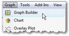
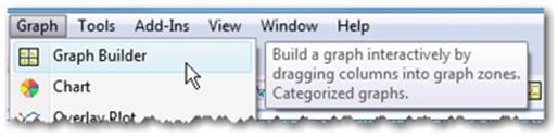
2. Open Graph Builder. Select Graph ▶ Graph Builder (see Figure 4.1).
Figure 4.1 Open Graph Builder
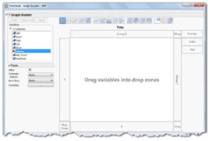
3. Notice the columns in your data table appear on the left in the Variables box (see Figure 4.2).
Figure 4.2 Graph Builder Variables
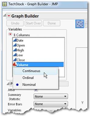
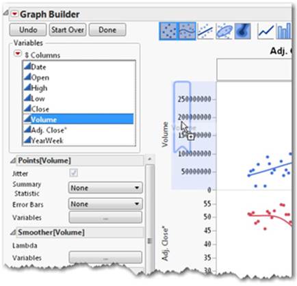
4. In the Variables box, change the Volume column from Nominal to Continuous by clicking on the icon in the Variables box on the left (as in Figure 4.3).
Figure 4.3 Change Volume from Nominal to Continuous
5. Drag the Adj. Close* column from the Variables box to one of the labeled zones located around the graph canvas. You will notice that as soon as the column is dragged into the zone, a graph of that data is immediately displayed. Keeping the mouse button depressed, experiment by dragging the column into different drop zones to see what happens. If you let go of the mouse button, you can always click the Undo or Start Over button to begin again.
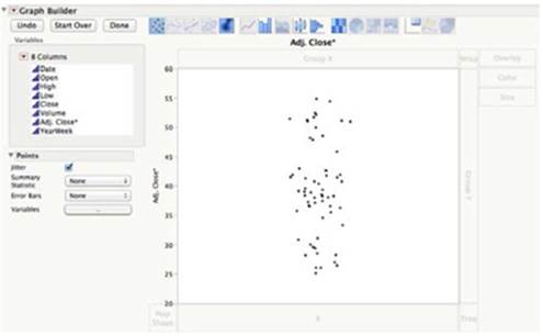
6. Click, hold, and Drag the Adj. Close* column to the Y drop zone and release the mouse button. You should see a point graph (see Figure 4.4).
Figure 4.4 Drag Adjusted Close to Y Drop Zone
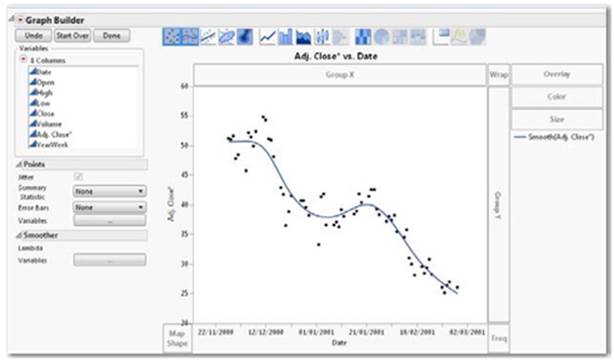
7. Now click and drag the Date column to the X drop zone. This action immediately produces a scatter plot with dates on the x-axis (see Figure 4.5). Notice that the trend for the close prices is downward and a smoothing line is fit to the data.
Figure 4.5 Drag Date to X Drop Zone
8. Right-click in the graph region to change the look of the graph (see Figure 4.6). A menu appears, containing options to make graph changes. Make no changes at this time. Additional visualization changes can be accomplished by choosing from the palette of icons across the top of the graph (see Figure 4.7). These are the Element Type Icons.
Figure 4.6 Right Mouse Click in the Graph Region
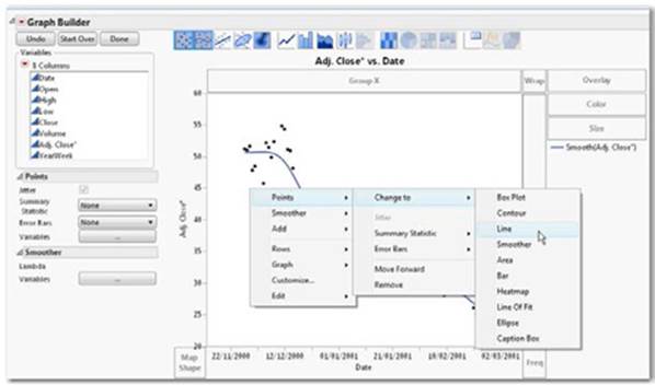
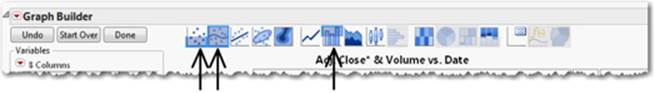
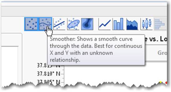
Figure 4.7 Element Type Icon Smoother
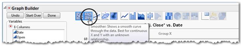
9. Select the icon that is second from the left on the palette of icons at the top (circled in Figure 4.7). This toggles the smooth curve on and off. Highlighted choices are enabled. Grayed out choices are disabled. Leave the smooth curve enabled.
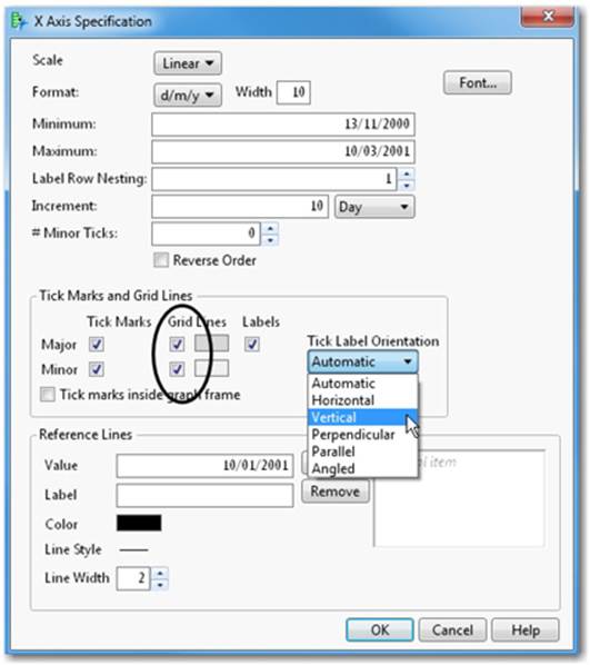
10. Now double-click on the Date axis. You see a window box of choices (see Figure 4.8). Change the Tick Label Orientation to Vertical. In Grid Lines, add a check for grid lines for the Major and Minor axes and click OK.
Figure 4.8 Change Tick Orientation and Gridlines
11. You should now see a graph with vertical dates and gridlines at the major tick date intervals. Now drag the Volume column to the area just above the y-axis label for Adj. Close* (see Figure 4.9).
Figure 4.9 Drag Volume to Y Drop Zone
12. You will see a graph rendered (see Figure 4.10).
Figure 4.10 Graph Rendered
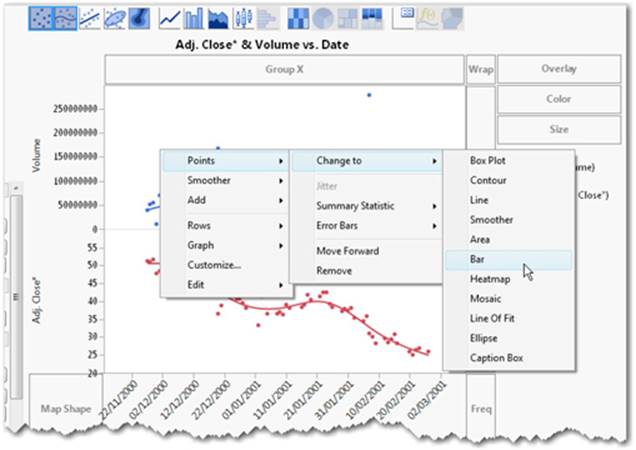
13. Right-click on the Volume graph points (see Figure 4.11), and select Points ▶ Change to ▶ Bar.
Figure 4.11 Change Points to Bars
Note that the Element Type Icons at the top of the chart give an iconographic indication of what parts of the graph elements are currently enabled (see Figure 4.12).
Figure 4.12 Element Type Icons
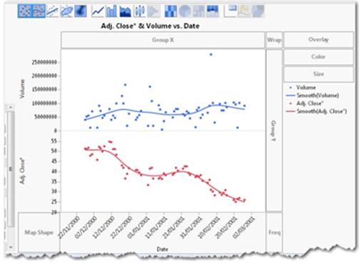
Elements of the graph’s rendering can be controlled from this panel. Reading the icons for the current graph from left to right, points are enabled for the Adj. Close* y-axis only (indicated by the lower half of the icon being highlighted and corresponding to the lower half of the graph in Figure 4.13). Smoother is enabled for both Adj. Close* and for Volume. Bars are enabled for Volume only (the upper half of the graph).
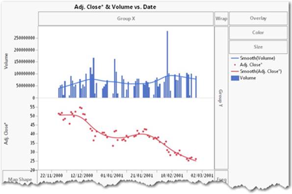
14. This renders a graph showing trading volume and adjusted closing prices for the time period (see Figure 4.13).
Figure 4.13 Enable Smoother for Volume and Adjusted Close
15. Now let’s include the daily high and low prices in the graph. Drag the High column to the location just to the right of the y-axis for Adj. Close* (see Figure 4.14).
Figure 4.14 Include Daily High and Low Prices
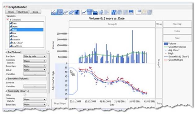
16. A red High line is now rendered that represents the maximum price of the stock portfolio by day. If you don’t get the picture to match Figure 4.14 the first time, you can always click undo and try again. Now do the same with the Low column by clicking and dragging the Lowcolumn to the same location. A green Low line is now rendered that represents the minimum price for each day.
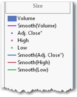
17. To complete the graph, edit the last few items. Double-click in the inside of the legend (see Figure 4.15).
Figure 4.15 Edit the Legend
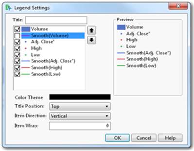
18. A Legend Settings window appears (see Figure 4.16).
Figure 4.16 Legend Settings Window
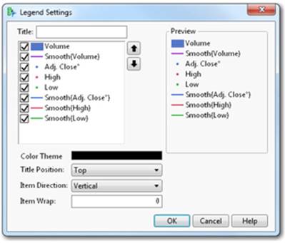
19. Click on the purple Volume line and remove the check mark for that item. Then click in the Preview area of the dialog box. The dialog box should look like Figure 4.17. Click OK.
Figure 4.17 Volume Line and Preview
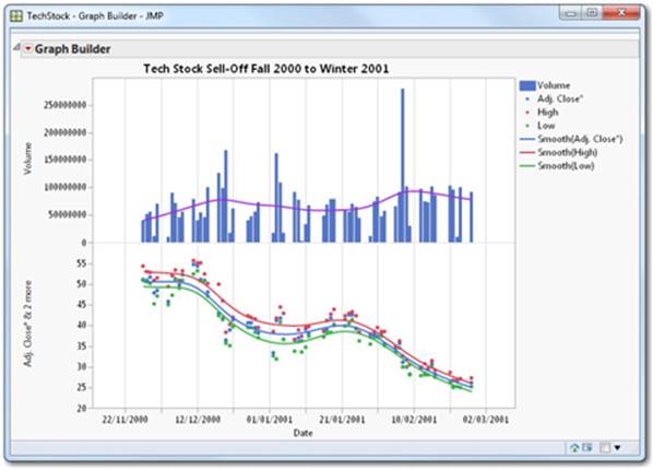
20. Now let’s add a few last details. We’ll change the graph title. Click on the graph title and change it to Tech Stock Sell-Off Fall 2000 to Winter 2001. Then click Done. You should see a graph like that in Figure 4.18.
Figure 4.18 Final Graph
4.2 Using Graph Builder to Produce Maps
The Graph Builder platform also enables you to visualize data on a map, even at the street level. In JMP, maps can be created two ways: using shape files (which are data tables containing the boundaries and names of the shapes such as states or counties of the USA) or background maps (which are background images that recognize latitude and longitude and allow you to plot points accordingly).
Today, mapping data is abundant; JMP provides an easy and flexible environment in which to convey your data on maps. The example below will illustrate how to create a thematic map using the background map service called OpenStreetMaps. An Internet connection is required to use OpenStreetMaps, and you must be using JMP 11 or later.
To make maps in Graph Builder, simply use the same drag and drop methods you practiced in the previous section. The key step is dragging a shape column to the Map Shape drop zone (to utilize a Shape file) or in using latitude and longitude data columns in the X and Y drop zones respectively (to utilize a background map). This action enables maps to be visualized with your columns of interest data.
If you are unfamiliar with the special conditions of how map data is handled in JMP see Section 2.7.
Example 4.2: San Francisco Crime
We’ll be working with one of the sample data files to illustrate the steps in this section. The file we’ll use, San Francisco Crime.jmp, which contains data on individual crime incidents in San Francisco from April 2012. You can find the data set at Help ▶ Sample Data ▶ Graph Builder ▶ San Francisco Crime.
The columns include:
Incident Number identifier represented as an integer
Date the date expressed as dd/mm/yyyy
Time hour and minute expressed as HH:MM: AM/PM
Day of Week day of the week expressed as a word
Category 32 offense categories, expressed as words
Incident Description 336 standardized sub categories of the Category column, expressed as words
Traffic Incident 2 categories standardized for indicators of traffic incident, expressed as words
Resolution 16 categories of standardized indicators of incident resolution, expressed as words
Police District 10 categories of geographic police district names in the city of San Francisco
Incident Address nearest cross-street
Longitude longitude expressed in degrees and directions east and west
Latitude latitude expressed in degrees and directions north and south
Reference a compact set of 4 hidden columns that automatically performs recoding
Police Department Color a row state column indicating a color marker indexed to each police district
1. First, open the sample data table by selecting Help ▶ Sample Data ▶ Graph Builder ▶ San Francisco Crime.
2. Open Graph Builder. Select Graph ▶ Graph Builder (see Figure 4.19).
Figure 4.19 Open Graph Builder
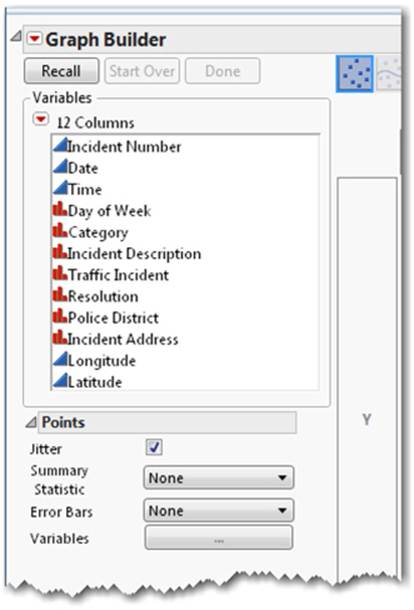
3. Notice the columns in your data table appear on the left in the Variables list (see Figure 4.20).
Figure 4.20 San Francisco Crime Variables
4. Now drag the Latitude column from the Variables list to the Y drop zone located in the graph canvas. Then drag the Longitude column from the Variables list to the X drop zone located in the graph canvas. You should see a point graph with a smoother line (see Figure 4.21).
Figure 4.21 Latitude and Longitude Point Graph
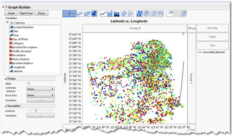
5. Let’s de-select the second icon on the element type palette by clicking on the icon to remove the smoother line from the graph (Figure 4.22).
Figure 4.22 Remove Smoother Line
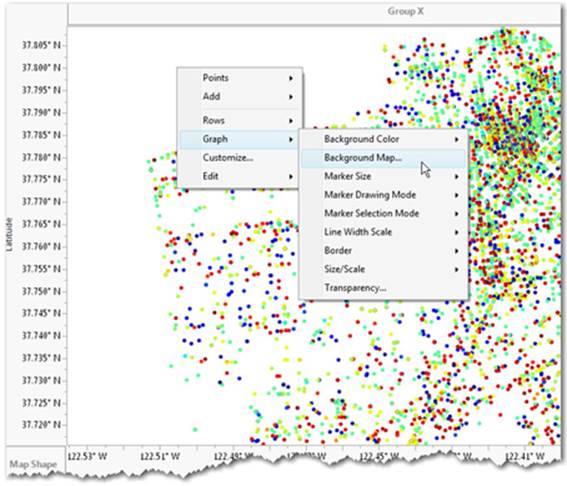
6. Now right-click in the middle of the graph area and choose Graphs ▶ Background Map from the submenu (see Figure 4.23).
Figure 4.23 Graph Builder Background Map
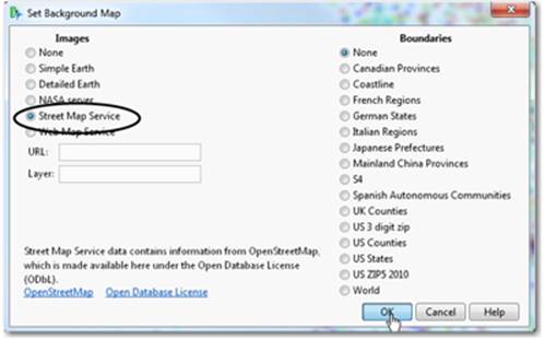
7. Select Street Map Service and click OK (see Figure 4.24).
Figure 4.24 Graph Builder Street Map Service
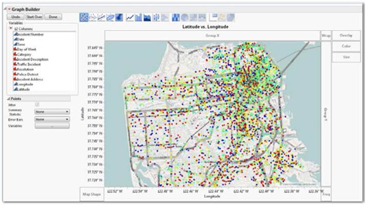
8. The addition of San Francisco streets now appear as a background to the color-coded crime locations (see Figure 4.25).
Figure 4.25 Background Street Map Overlay—Color-Coded Crimes
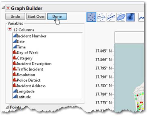
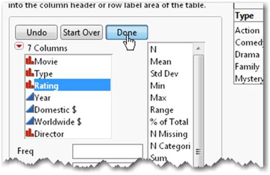
9. You are now finished with the Variables control panel. Click the Done button from the control panel to close the panel (see Figure 4.26).
Figure 4.26 Close the Variables Control Panel
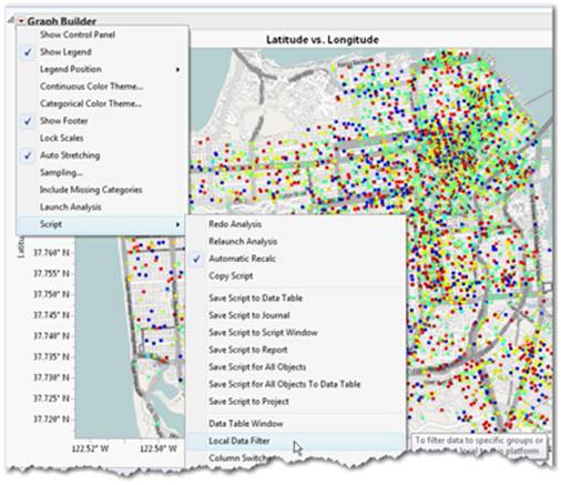
10. Now let’s focus on assaults in one particular police district. To do this, we will use a powerful feature called the Local Data Filter. From the red triangle for Graph Builder, choose Script ▶ Local Data Filter (see Figure 4.27).
Figure 4.27 Select Local Data Filter
11. A Local Data Filter panel appears to the left and inside the Graph Builder window (see Figure 4.28).
Figure 4.28 Local Data Filter Panel
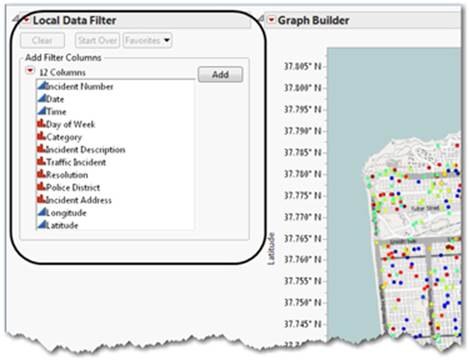
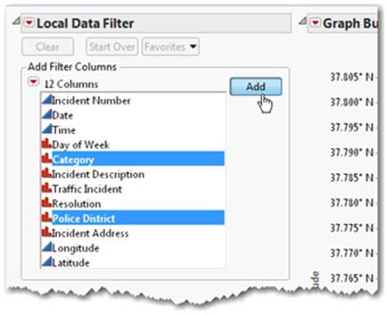
12. Hold down the Ctrl key, select Category and Police District and then click the Add button (see Figure 4.29).
Figure 4.29 Data Filter Category and Police District
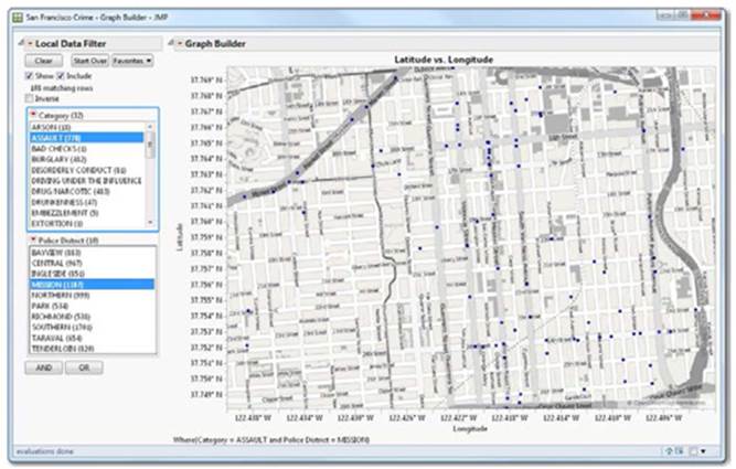
13. A list of crimes and police districts appears in the local data filter. Select ASSAULT from the Category list, hold down the CTRL key and select MISSION from the Police District list. The map automatically zooms to the Mission District and maps assault crimes as blue dots (see Figure 4.30).
Figure 4.30 Data Filter Assault and Mission
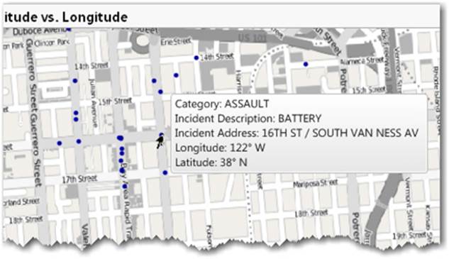
14. Now move your mouse pointer and hover over any of the blue dots. Labeling information for the crime is automatically displayed (see Figure 4.31).
Figure 4.31 Display Label Information
Note: Column information may be used as labels by turning on the label property in the columns list in the data table. If labeling columns is unfamiliar to you, see “Adding Labels to Data” in Chapter 2.
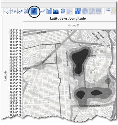
15. Now, let’s add contours to this map. Contours will help to plot the density of assaults for the Mission District in San Francisco during this time period. From the red triangle for Graph Builder, select Graph Builder ▶ Control Panel. Hold the Shift key and select the contour icon (circled in Figure 4.32).
Figure 4.32 Add Contours for Density of Assaults
16. Many additional visualizations are possible. Feel free to experiment. You can always click the Undo button if you want to go back. Click the Done button when you are finished.
4.3 Using Tabulate
Now that you are familiar with using drop zones to generate a graph, we introduce the Tabulate platform. Tabulate is used in a similar fashion to Graph Builder, but instead of creating graphs, your objective is to create numerical summaries for their own sake or for the development of new data tables based on summarized data for further analysis.
Example 4.3: Movies
We’ll use Movies.jmp to demonstrate Tabulate. This data table is a listing of popular US movies that were released between 1937 through 2003. The movies are categorized by type, rating, and director and contain earned gross dollar amounts for both the US domestic market and the worldwide market. Note: Dollar amounts are expressed in millions of dollars for both domestic and worldwide markets.
You can find the data set at Help ▶ Sample Data ▶ Business and Demographic ▶ Movies.
The columns include:
Movie name of movie
Director director of movie
Type genre/category of movie (for example: comedy, family)
Rating US movie rating system (for example: general audience [G], adult [R])
Year year of movie release (for example: 1937)
Domestic $ US domestic revenue in $ earned by the movie in that year
Worldwide $ Worldwide revenue in $ earned by the movie in that year
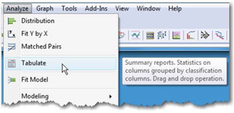
1. After opening the data table, open Tabulate (select Analyze ▶ Tabulate) (see Figure 4.33).
Figure 4.33 Open Tabulate Platform
2. The Tabulate platform presents a control panel with your columns, a statistics list, and drop zones for rows and columns (see Figure 4.34)
Figure 4.34 Tabulate with Domestic and Worldwide Columns
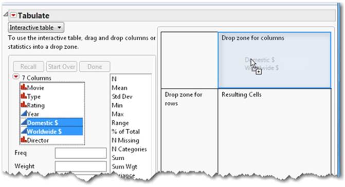
3. Click on both the Domestic $ and Worldwide $ columns and drag them to the part of the table labeled Drop zone for columns (see Figure 4.34).
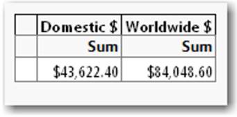
4. A sum of movie revenue by domestic $ and worldwide $ appears (see Figure 4.35).
Figure 4.35 Sum of Domestic and Worldwide Movie Revenue
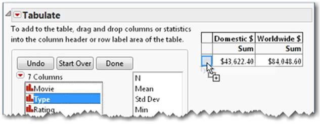
5. Now drag the Type column to the row area (see Figure 4.36).
Figure 4.36 Drag Type Column to Row Area
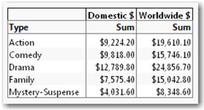
6. Release the mouse button; the table now sums the revenue by type for both domestic and worldwide (see Figure 4.37).
Figure 4.37
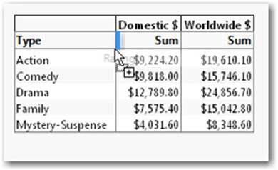
7. We would like to add a Rating subgroup within the Type column. Drag the Rating column to the area just to the left of the Domestic Sum column (see Figure 4.38).
Figure 4.38 Add Rating Subgroup Within Type Column
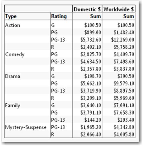
8. Release the mouse button and a Rating column appears (see Figure 4.39).
Figure 4.39 Table with Rating Column Added
Note: You can click the Undo button at any time to undo the last action, or you can click Start Over to start over again.
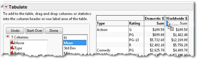
9. Drag the Mean from the Statistics column and drop it on one of the Sum column headings (see Figure 4.40).
Figure 4.40 Drag Mean Column to Sum Column
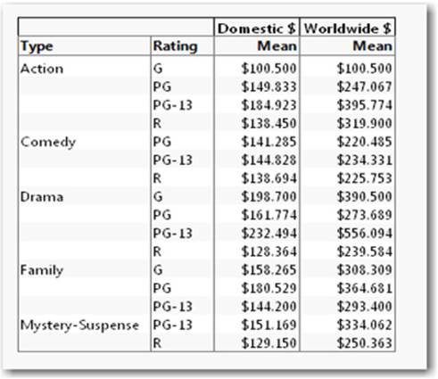
10. Then, release the mouse button. The Sum columns have been transformed to Mean columns (see Figure 4.41).
Figure 4.41 Sum Columns Changed to Mean Columns
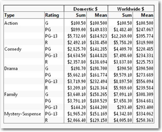
11. Now drag the Sum statistic to the right of the Domestic $, Mean column (see Figure 4.42). Then, release the mouse button. Sum columns then reappear in the table (see Figure 4.43).
Figure 4.42 Drag Sum Column to the Right of Domestic $ Column
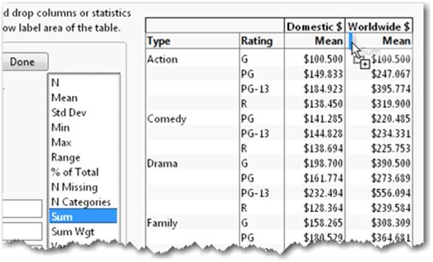
Figure 4.43 Sum Column Added
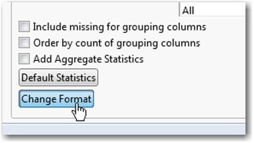
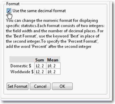
12. The decimal and display formats can be changed. In the previous example, there are three decimals displayed to the right of the decimal point for the Mean column. We would like to display only two decimal places for values in the table. To adjust the display of decimals, clickChange Format (see Figure 4.44a).
4.44a Change Format
13. An additional format panel appears. In the format pane, enter a 2 for the Mean column for both Domestic $ and Worldwide $ so the panel looks as it is shown (see Figure 4.44b).
Figure 4.44b Change Decimal Display
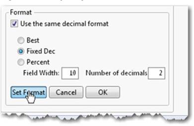
Click the Set Format button. Select the check box for Use Same Decimal format for all. The window changes (see Figure 4.44c). Click Fixed Dec and enter a 2 for Number of Decimals. Then, click Set Format and OK.
Figure 4.44c Specify Fixed Decimal Width
14. The table is now complete. Click Done (see Figure 4.45).
Figure 4.45 Finalize Changes
15. Recall that additional options are available on the red triangle. Click the red triangle next to Tabulate and select Make Into Data Table (see Figure 4.46), which will produce a JMP data table of the Tabulate results (see Figure 4.47). Make Into Data Table will accomplish two tasks simultaneously; you will have a summary table for reporting and a data table of summarized data ready for further analysis or visualization.
Tabulate, therefore, is a useful tool for reshaping and reorganizing data for further analysis or graphing in addition to producing tabular reports.
Figure 4.46 Make Data Table from Tabulate Results
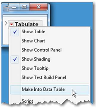
Figure 4.47 Newly Created Data Table
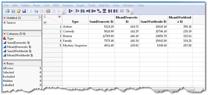
What do you think you can do with the new table in Figure 4.47? Try putting your new skills to work. Use Graph Builder to make a graph out of the data table you just produced (select Graph ▶ Graph Builder).
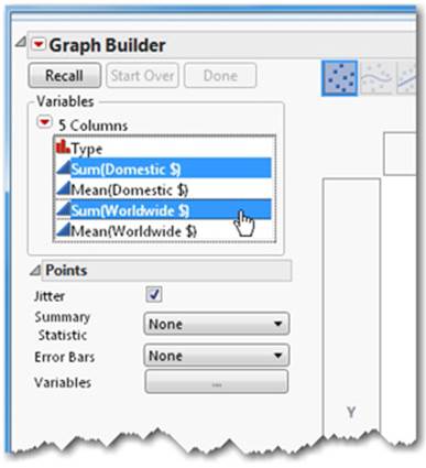
16. Now, press CTRL and select the columns Sum (Domestic $) and Sum (Worldwide $) so that they are both highlighted (see Figure 4.48).
Figure 4.48 Select Sum Columns
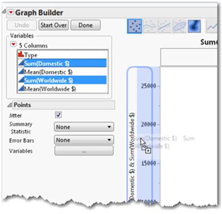
17. Drag the two selected columns to the Y drop zone (see Figure 4.49).
Figure 4.49 Drag Sum Columns to Y Drop Zone
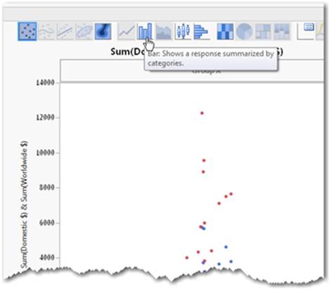
18. A point chart initially appears with blue and red dots. Select the Bar element type icon (see Figure 4.50). Note: Of course, you could right click in the graph as you learned earlier in the chapter.
Figure 4.50 Convert Point Chart to Bar Chart
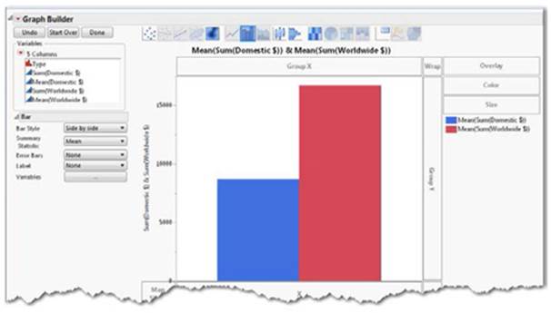
19. A bar chart appears, showing the worldwide and domestic revenue comparisons (see Figure 4.51).
Figure 4.51 Bar Chart
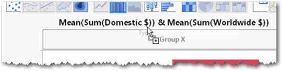
20. Now, drag Type to the Group X drop zone (see Figure 4.52).
Figure 4.52 Drag Type to Group X Drop Zone
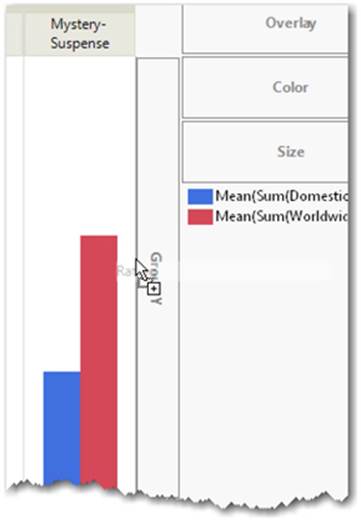
21. Now, drag Rating to the Group Y drop zone (see Figure 4.53).
Figure 4.53 Drag Rating to Group Y Drop Zone
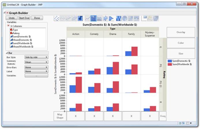
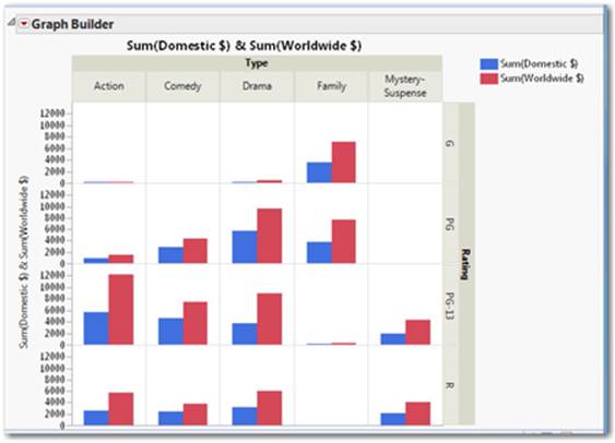
22. The nearly finished graph appears (see Figure 4.54).
Figure 4.54 Nearly Finished Graph
23. Click Done, and the finished graph appears (see Figures 4.55 and 4.56).
Figure 4.55 Click Done to Fnalize
Figure 4.56 Final Graph
4.4 Summary
In this chapter, we examined a key feature of JMP, which is its ability to create graphs and summaries interactively and intuitively in an environment that enables quick exploration and discovery. This chapter introduced you to two tools, Graph Builder and Tabulate.
Graph Builder shows you quick previews of graphs and maps as you drag columns to drop zones, enabling you to flip through choices until you find just the right one to tell the graphical story in your data. With a local data filter, Graph Builder allows you to drill down to the right level in your data. Contrast using Graph Builder to the methods employed in Chapter 3, where it is assumed that you have a specific graph in mind and need directions to reproduce it.
Tabulate shows you quick previews of numerical table summaries as you drag columns to drop zones. Tabulate enables you to flip through choices until you find the right numerical table summary of your data.
All materials on the site are licensed Creative Commons Attribution-Sharealike 3.0 Unported CC BY-SA 3.0 & GNU Free Documentation License (GFDL)
If you are the copyright holder of any material contained on our site and intend to remove it, please contact our site administrator for approval.
© 2016-2026 All site design rights belong to S.Y.A.