Using JMP 12 (2015)

Appendix A. Formula Functions Reference

Descriptions of Functions in the Formula Editor

You can add functions to a formula. All of these functions are organized in the function browser, which groups collections of functions and features in lists organized both alphabetically (Functions (all)) and by topic (Functions (grouped)). This chapter gives a description of functions in the Formula Editor.

More information about functions is available in the following resources:

•Scripting Index describes all functions and their arguments, demonstrates how the functions work, and links to online Help. In JMP, select Help > Scripting Index to view this interactive resource.

•The Scripting Guide also provides the arguments for all JMP functions, not just those available in the Formula Editor. In JMP, select Help > Books > Scripting Guide to open a PDF of the Scripting Guide.

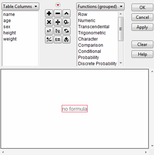
Figure A.1 Functions in the Formula Editor

For instructions on how to create a formula that contains a function, see “Create a Formula” in the “Formula Editor” chapter.

Contents

Row Functions

Numeric Functions

Transcendental Functions

Trigonometric Functions

Character Functions

Character Pattern Functions

Comparison Functions

Conditional Functions

Probability Functions

Discrete Probability Functions

Statistical Functions

Random Functions

Date Time Functions

Row State Functions

Assignment Functions

Parametric Model Functions

Finance Functions

Row Functions

Adding a row function to a formula lets you reference specific rows or cells within specific rows. You can also insert values based on an arithmetic sequence. See the Scripting Guide for details about syntax.

Sequence

Produces an arithmetic sequence of numbers across the rows in a data table, where the start value, ending limit, and increment are specified as arguments.

Count

Creates a list of values beginning with the from value and ending with the to value. The number of steps specifies the number of values in the list between and including the from and to values. Each value determined by the first three arguments of the count function occurs consecutively the number of times that you specify with the times argument. When the to value is reached, Count starts over at the from value.

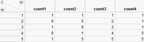
Also, you can add the times argument with the insert button on the keyboard. This argument is one by default, but repeats the count process as many times as you specify, as illustrated by the Count4 column in the data table in Figure A.2. To add any argument to the Count function, highlight the argument preceding the one that you want to enter. Either type a comma or use the insert button on the Formula Editor keypad.

The columns in the data table below result from the following formulas:

•Count (1, 9, 2) gives Count 1

•Count (1, 9, 3) gives Count 2

•Count (1, 9, 9) gives Count 3

•Count (1, 9, 3, 3) gives Count 4

Figure A.2 Example of the Count Function

The Count function is useful for generating a column of grid values. For example, the following formulas create a square grid of increment NRow(). NRow() is the Row function that gives the total number of rows in the data table) and axes that range from –5 to 5:

Count (–5, 5, Root(NRow()))

Count (–5, 5, Root(NRow()), Root(NRow()))

Lag

Returns the value of the first argument in the row defined by the current row less the second argument. The default Lag is one, which you can change to any number. The value returned for any lag that identifies a row number less than one is missing. Note that Lag(X, n) gives the same result as the subscripted notation, X_{Row( )–n}.

Dif

Returns the difference between the value of the first argument in the current row and its value in the row defined by the current row less the second argument. The default Dif is one, which you can change to any number. Note that Dif(X, n) gives the same result as X_Row()–X_Row()-n, or asX_Row()–Lag(X, n).

Subscript

Enables you to use a column’s value from a row other than the current row. After choosing Subscript from the list, enter a numeric expression into the subscript argument. Subscripts that evaluate to nonexistent row numbers produce missing values. Column names with no subscript refers to the current row. To remove a subscript, select the subscript and delete it. Then delete the missing box.

The formula Count_Row() – Count_Row()–1, where Row() is the row number as described below, uses subscripts to calculate the difference between each pair of values from the column named Count. This result is the same as that given by the Dif() function. When Row() is 1, the computation produces a missing value.

The formula below calculates a column called Fib, which contains the terms of the Fibonacci series (each value is the sum of the two preceding values in the calculated column).

It shows the use of subscripts to do recursive calculations. A recursive formula includes the name of the calculated column, subscripted such that it references only previously evaluated rows (rows 1 through (i–1)). The calculation of the Fibonacci series shown includes a conditional expression and a comparison. See the sections “Conditional Functions”, and “Comparison Functions”, for details.

Row

Returns the current row number when an expression is evaluated for that row. You can use Row() in any expression, including column name subscripts. The default subscript of a column name is Row() unless otherwise specified.

NRow

Returns the total number of rows in the active data table.

Numeric Functions

You can create a formula that contains arithmetic operators that are commonly used in formulas. See the Scripting Guide for details about syntax.

Abs

Returns a positive number of the same magnitude as the value of its argument. For example, |5| and |–5| both result in 5.

Modulo

Returns the remainder when the second argument is divided into the first. For example, Modulo(6, 5) results in 1.

Ceiling

Returns the smallest integer greater than or equal to its argument. For example, Ceiling(2.3) results in 3, while Ceiling(–2.3) results in –2.

Floor

Returns the largest integer less than or equal to its argument. For example, Floor(2.7) results in 2, but Floor(–0.5) results in –1.

Round

Rounds the first argument to the number of decimal places given by the second argument. For example, Round(3.554, 2) rounds to 3.55 and Round(3.555, 2) rounds to 3.56.

Transcendental Functions

You can create a formula that supports transcendental functions, such as logarithmic functions for any base, functions for combinatorial calculations, the Beta function, and several gamma functions. See the Scripting Guide for details about syntax.

Exp

Raises e to the power that you specify. Thus, Exp(1) = e.

LnZ

Calculates the natural logarithm of x, except returns 0 when x is 0; for use with derivatives.

Log and Log10

Calculates the natural logarithm (base e). To change the default base, highlight the argument and type a comma or click the insert key on the keypad. The base appears and is editable. The Log argument can be any numeric expressions. The expression Log(e) evaluates as 1, and Log2(32) is 5. The Log10 function calculates the logarithm of base 10 only.

Log1P

Returns a more accurate calculation of Log(1+x) when x is very small.

Squash

Computes the function 1 / (1 + e^x), where x is any numeric column, variable, or expression.

Logist

Also known as Squish or Logistic, is an efficient computation of the function 1 / (1+e^-x), where x is any numeric column, variable, or expression.

Root or Square Root

Calculates the root of its argument as specified by the index. Root initially shows with an index of 2. To change the index, highlight the index argument and enter the value that you want.

Factorial

Returns the product of all numbers 1 through the argument that you specify. For example, Factorial(5) evaluates as 120.

NChooseK

Returns the number of n things taken k at a time (n select k) and is computed in the standard way using factorials, as n! / (k!(n – k)!). For example, NChooseK(5,2) evaluates as 10.

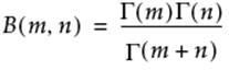
Beta

Adds the two parameter Beta function and is written terms of the Gamma function as:

Gamma

Adds the Gamma function, denoted Γ(i), and is defined as:

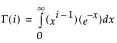
Gamma with a single argument is the same as Gamma(x, infinity). The optional second argument changes the upper integer from infinity to the value that you enter. Other interesting gamma function relationships are

•for any α > 1, Γ(α) = (α–1) • Γ(α–1)

•for any positive integer, n, Γ(n) = (n-1)!

•Γ(0.5) = the square root of π

LGamma

Is the natural log of the result of the gamma function evaluation. You get the same result using the Log (natural log) function with the Gamma function. However, the LGamma function computes more efficiently than do the Log (natural log) and the Gamma functions together.NChooseK is implemented using LGamma functions. The result is not always an exact integer. If the result is close to an integer, it is rounded up using the Floor function.

Digamma

The logarithmic derivative of the Gamma function.

Trigamma

The derivative of the Digamma function, or the logarithmic second derivative of the Gamma function.

Arrhenius

Calculates the non-specific component of the Arrhenius relationship that is then multiplied by the activation energy in the Arrhenius equation.

Arrhenius Inv

The inverse of the Arrhenius function:

Logit

Applies the logit transformation to the argument using:

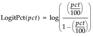
Logit Percent

Calculates the logit as a percent for the argument.

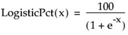
Logist Percent

Calculates the logistic as a percent for the argument.

Scheffe Cubic

Is used in fitting certain models. Scheffe Cubic (X1, X2) is equivalent to X1*X2*(X1-X2).

Trigonometric Functions

You can create a formula that supports transcendental functions, such as logarithmic functions for any base, functions for combinatorial calculations, the Beta function, and several gamma functions. See the Scripting Guide for details about syntax.

Sine, Cosine, Tangent

The Sine and Cosine functions calculate the sine and cosine of their respective arguments given in radians. For example, the expression Sine(0) evaluates as 0, and Cosine(0) evaluates as 1. The tangent function calculates the tangent of an argument given in radians. The expressionTan(Pi()/4) evaluates as 1.

ArcSine, ArcCosine, ArcTangent

The ArcSine and ArcCosine functions return the inverse sine and inverse cosine of their respective arguments. The returned value is measured in radians. For example, both expressions ArcSine(1) and ArcCosine(0) evaluate as 1.57080. The ArcTangent function returns the inverse tangent of its argument. The returned value is measured in radians. The expression ArcTangent(1) evaluates as 0.78540 (=3.14159/4).

SinH, CosH, TanH

The SinH and CosH functions return the hyperbolic sine and hyperbolic cosine of their respective arguments. The expression SinH(1) evaluates as 1.175201, and CosH(0) evaluates as 1.0. The TanH function returns the hyperbolic tangent of its argument. The expression TanH(1)evaluates as 0.761594.

ArcSinH, ArcCosH, ArcTanH

The ArcSinH and ArcCosH functions return the inverse hyperbolic sine and inverse hyperbolic cosine of their respective arguments. The expression ArcSinH(1) evaluates as 0.881374, and ArcCosH(1) is 0. The ArcTanH function returns the inverse hyperbolic tangent of its argument. The expression ArcTanH(0.5) evaluates as 0.549306.

Character Functions

You can create a formula that accepts character arguments or returns character strings and converts the data type of a value from numeric to character, or character to numeric. When you create these formulas, note that:

•Character functions can result in either character or numeric data. If you calculate a data type different from the one specified, the data type of the computed column is automatically changed to match the result.

•Arguments that are literal character strings must be enclosed in quotation marks.

See the Scripting Guide for details about syntax.

Char

Produces a character string that corresponds to the digits in its numeric argument. For example, Char(1.123) evaluates as 1.123. See the Scripting Guide, for details.

Collapse Whitespace

Trims leading and trailing whitespace and replaces interior whitespace with single space. That is, if more than one white space character is present, the Collapse Whitespace command replaces the two spaces with one space.

Concat ||

Concatenates character strings to produce a new string with the function’s second character argument appended to the first. For example, "Dr." || " " || name produces a new string consisting of the title Dr. followed by a space and the contents of the name string. (See also “Concat Items”.)

Contains

Returns the numeric position within the first argument of the first instance of the second argument, if it exists. The second argument can contain one ore more characters. If the second argument does not exist, Contains returns a zero. For example, Contains("Veronica Layman", "ay")evaluates as 11. Contains("Lillie Layman", "L") evaluates as 1. The third argument is optional and is a numeric value that specifies the starting position. If offset is negative, Contains searches backward from offset from the end of the string.

Munger

Computes new character strings from existing strings by inserting or deleting characters. It can also produce substrings, calculate indices, and perform other tasks depending on how you specify its arguments. The Munger function treats uppercase and lowercase letters as different characters.

Text is a character expression. Munger applies the other three arguments to this string to compute a result.

Offset is a numeric expression indicating the starting position to search in the string. If Offset is greater than the position of the first instance of the find argument, the first instance is disregarded.

Find/Length is a character or numeric expression. Use a character string as search criterion, or use a positive integer to return that number of consecutive characters starting from the Offset position. If you specify a negative integer as the Length value, Munger returns all characters from the Offset through to the end of the string.

Replace (optional argument) can be a string or unspecified. If it is a string and the Find/Offset value is numeric, Munger replaces the search criterion with the Replace string to form the result. If the Find/Offset value is numeric and no string is specified, Munger calculates a substring. If the Find/Length value is a character string, Munger always returns the numeric offset, disregarding the Replace value if it exists. To insert the Replace argument, click any argument in the Munger function and then click the insert button. Use the delete key on your keyboard or the delete button () on the Formula Editor keypad to remove the Replace argument.

Lowercase, Uppercase

The Lowercase function converts any uppercase character found in its argument to the equivalent lowercase character. For example, Lowercase("VERONICA LAYMAN") evaluates as veronica layman. The Uppercase function converts any lowercase character found in its argument to the equivalent uppercase character. For example, Uppercase("Veronica Layman") evaluates as VERONICA LAYMAN.

Length

Calculates the length of its argument. For example, Length("Veronica") evaluates as 8. If the argument is

•a string, length returns the number of characters;

•a list, length returns the number of items in the list;

•a blob (binary object), the number of bytes.

Num

Produces a numeric value that corresponds to its character string argument when the character string consists of numbers only. If a character string contains a non-numeric value, the result is a missing value. For example, Num(“1.123”) evaluates as 1.123.

Substr

Extracts the characters that are the portion of the first argument. Begins at the position given by the second argument, and ends based on the number of characters specified in the third argument. The first argument can be either a character column or a literal value. The starting argument and the length argument can be numbers of expressions that evaluate to numbers. For example, to show the first name only, Substr("Veronica Layman", 10, 6) starts at position 10 and reads through position 15, which yields Layman.

If start is negative, Substr searches backward from start from the end of the string. If length is negative or absent, Substr returns a string that begins with start and continues to the end of the text string.

Substr can also be used with lists.

Titlecase

Converts the string to title case, that is, an initial uppercase character and subsequent lowercase characters. For example, Titlecase(“Veronica Layman”) results in Veronica layman.

Trim

Produces a new character string from its argument, removing any leading and trailing whitespace. The second argument determines if whitespace is removed from the left, the right, or both ends of the string. If no second argument is used, whitespace is removed from both ends. For example, Trim("john ") evaluates as john. Trim(" john ", both) also evaluates as john.

Word

Extracts the n^th word from a character string. One or more spaces define where each word begins and ends unless the optional delimiters argument is specified. For example, Word(2, "Veronica Layman") returns the word Layman.

To insert the delimiters argument, click on any argument in the Word function and then click the insert button on the Formula Editor keypad. Use the delete key on your keyboard or the delete button on the Formula Editor keypad to remove the delimiters argument. If you do not specify a delimiter, space is used as the delimiter. If you define the delimiter as an empty string, each character is treated as a separate word.

Most special characters act as single delimiters. You can enter any character or set of characters to act as a word delimiter. For example, to extract the last name in the following example, use a comma and blank together as the delimiting characters and ask for the first word. Word(1, "Layman, Veronica", ", ") returns the word Layman.

Words

Extracts the words from text according to the delimiters listed in the optional second argument. The default delimiter is space. For example, Words("the quick brown fox") returns {"the","quick","brown","fox"}.

If you include a second argument, any and all characters in that argument are taken to be delimiters. For example, Words("Doe, Jane P.",", .") returns {"Doe","Jane","P"}.

To insert the delimiters argument, click on any argument in the Words function and then click the insert button on the Formula Editor keypad. Use the delete key on your keyboard or the delete button on the Formula Editor keypad to remove the delimiters argument. If you do not specify a delimiter, white space is used as the delimiter. If you define the delimiter as an empty string, each character is treated as a separate word.

Left, Right

Returns a substring of the left-most or right-most n characters of the string text, respectively. Both functions also work with lists.

Starts With, Ends With

Returns 1 if whole begins or ends with part, respectively. Returns 0 otherwise. Both functions also work with lists.

Item

Is different than the Word function because of the way it treats word delimiters. If a delimiter is found multiple times, or you enter a delimiter with multiple characters, the Word function treats them as a single delimiter. The Item function uses each delimiter to define a new word position. To compare, suppose a name is of the form lastname, firstname. The delimiter is a comma followed by a blank, such as:

Item(2, "Layman, Veronica", ", ")

Word(2, "Layman, Veronica", ", ")

The Item function returns a missing value because it treats the comma and blank separately and finds nothing between them. The Word function treats the comma and blank as a single delimiter and finds Veronica as the second word.

If you do not specify a delimiter, white space (blank space) is used as the delimiter. If you define the delimiter as an empty string, each character is treated as a separate item.

Char to Hex, Hex, Hex to Char, Hex to Number

Converts between Hex and other formats.

Hex returns the hexadecimal representation of its argument. If the argument is character (in quotes), then the result is a character string twice as long containing the hexadecimal codes for the character values. For example, Hex("A") returns the string 41.

If the argument is numeric and “integer” is specified, the Hex function returns an 8-hexadecimal-character representation of the integer returned. For example, Hex(12, “integer”) returns the string 0000000C.

Hex to Char converts hexadecimals to characters. The resulting character string might not be valid display characters. All the characters must be in pairs, in the ranges 0-9,A-Z, and a-z. Blanks and commas are allowed and skipped.

Char to Hex converts characters to hexadecimals.

Hex to Number converts hexadecimals to numbers.

For details, see the Scripting Guide book.

Repeat

Creates a string that is the first argument repeated the number of times specified by the second argument. The first argument can be either a character literal, a character variable, or a character expression. For example, Repeat(“Katie”, 3) creates KatieKatieKatie.

A third argument applies when Repeat is used in a JSL script to repeat a matrix. When the first argument is a matrix, the second argument is the rowwise repeat and the third argument is the columnwise repeat.

Insert, Insert Into

Insert inserts a new item into the list or expression at the given position. If position is not given, it is inserted at the end.

Insert Into is the same as insert, but it inserts in place.

Remove, Remove From

Remove the character(s) at the indicated position. If n is omitted, the item at position is deleted. If position and n are omitted, the item at the end is removed. There are three possible arguments: the string, followed by the position, followed by the number of characters to be removed.

Remove From returns items removed in place. The function returns the removed item(s), but you do not have to assign them to anything. The first argument is a variable name, followed by the position, followed by the number of characters to be removed.

Shift, Shift Into

Shift shifts an item or n items from the front to the back of the list or expression. Shifts items from back to front if n is negative. Shift Into shifts items in place.

Reverse, Reverse Into

Reverse reverses the characters in the string. Reverse Into reverses the characters in place.

Concat Items

Concat Items converts a list of string expressions into one string, with each item separated by a delimiter. The delimiter is a blank, if unspecified.

Substitute, Substitute Into

The first argument is a string, the second is a pattern, and the third is a replacement string. Substitute finds all matches to the pattern in the string, and replaces them with the replacement string. Substitute Into does the same substitution in place.

Regex

The first argument is the source string that Regex searches for a match to the pattern. The second argument is the pattern, in the form of a regular expression. The Formula Editor prompts you for these two required arguments.

Tip: For more information about using regular expressions, search the Internet for regular expression tutorial.

By default, Regex performs a case-sensitive search and returns the parts of the source string that match the pattern that you specified (or returns MISSING if the match fails). There are two optional arguments that you can add. You can type a third argument—the format—that specifies the string to return. If you choose, you can use regular expressions to specify replacement text in the returned string. If you specify the third argument, you can also specify IGNORECASE so that Regex ignores capitalization when searching the source string for a match.

For more information and an example that you can run, select Help > Scripting Index and do a search for Regex.

XPath Query

XPath Query parses a valid XML document for the expression that you specify. For an example, select Help > Scripting Index and search for the function.

Hex to Blob, Char to Blob, Blob to Char

Hex to Blob converts the hexadecimal to a blob (Binary Large Object).

Char to Blob converts the string to a blob. You can specify the encoding in an optional second argument. Supported encodings are: utf-8, utf-16le, utf-16be, us-ascii, iso-8859-1, and ascii~hex.

Blob to Char converts the blob to a string. You can specify the encoding in an optional second argument. Supported encodings are: utf-8, utf-16le, utf-16be, us-ascii, iso-8859-1, and ascii~hex.

Character Pattern Functions

These functions provide powerful pattern matching abilities. Pattern matching is a flexible method for searching and manipulating strings, and regular expressions are also supported. When you create these formulas, note that:

•First, you define a pattern with one more of the character patterns.

•Then, you use Pat Match to compare a string to the pattern.

•Pat Match returns True (1) if the pattern is found in the string, or it returns False (0) if the pattern was not found in the string.

•To use regular expressions instead of patterns, use Regex Match.

For complete details, see the Scripting Guide.

Pat Any

Constructs a pattern that matches a single character in the argument.

Pat Not Any

Constructs a pattern that matches a single character that is not in the argument.

Pat Break

Constructs a pattern that matches zero or more characters that are not in its argument; it stops or breaks on a character in its argument. It fails if a character in its argument is not found. In particular, it fails to match if it finds the end of the source string without finding a break character.

Pat Span

Constructs a pattern that matches one or more (not zero) occurrences of characters in its argument. It is greedy; it always matches the longest possible string. It fails rather than matching zero characters.

Pat String

Constructs a pattern that matches its string argument.

Pat Len

Constructs a pattern that matches n characters.

Pat Pos

Constructs patterns that match the null string if the current position is int from the left end of the string, and fail otherwise.

Pat R Pos

Constructs patterns that match the null string if the current position is int from the right end of the string, and fails otherwise.

Pat Tab

Constructs a pattern that matches forward to position int in the source string. It can match 0 or more characters. It fails if it would have to move backwards or beyond the end of the string.

Pat R Tab

Constructs a pattern that matches up to position n from the end of the string. It can match 0 or more characters. It fails if it would have to move backwards or beyond the end of the string.

Pat Test

Constructs a pattern that succeeds and matches the null string if expr is not zero and fails otherwise.

Pat At

Constructs a pattern that matches the null string and stores the current position in the source string into the specified JSL variable (varName). The assignment is immediate, and the variable can be used with expr() to affect the remainder of the match.

Pat Rem

Constructs a pattern that matches the remainder of the string. It is equivalent to patRTab(0).

Pat Arb

Constructs a pattern that matches an arbitrary string. Initially it matches the null string. It matches one additional character each time the pattern matcher backs into it.

Pat Succeed

Constructs a pattern that always succeeds, even when the matcher backs into it. It matches the null string.

Pat Fail

Constructs a pattern that fails whenever the matcher attempts to move forward through it. The matcher backs up and tries different alternatives. If and when there are no alternatives left, the match fails and Pat Match returns 0.

Pat Abort

Constructs a pattern that immediately cancels the pattern match. The matcher does not back up and retry any alternatives. Conditional assignments are not made. Immediate assignments that were already made are kept.

Pat Fence

Constructs a pattern that succeeds and matches the null string when the matcher moves forward through it, but fails when the matcher tries to back up through it. It is a one-way trap door that can be used to optimize some matches.

Pat Arb No

Constructs a pattern that matches zero or more copies of pattern.

Pat Repeat

Matches pattern between minimum and maximum times.

Pat Conditional

Saves the result of the pattern match, if it succeeds, to a variable named as the second argument (type) after the match is finished.

Pat Immediate

Saves the result of the pattern match to a variable named as the second argument (varName) immediately.

Pat Altern

Constructs a pattern that matches any one of the pattern arguments.

Pat Concat

Constructs a pattern that matches each pattern argument in turn.

Pat Regex

Constructs a pattern that matches the regular expression in the quoted string argument.

Pat Match

Pat Match executes a pattern match using the source in the first argument and the pattern in the second argument. The pattern must be constructed first, either inline or by assigning it to a JSL variable elsewhere. A third argument, if present, is the replacement text for the matched characters in the source argument (if the source argument is a variable). Pat Match returns true if the match succeeds. Additional arguments, in any order, are ANCHOR (match must begin at start of source), FULLSCAN (turn off some optimizations for special situations), and MATCHCASE (by default, A == a).

Pat Match returns true or false rather than a string, so Pat Match is somewhat difficult to use in a formula. You might find the Regex function (“Regex”) easier to use when you are adding pattern-matching formulas in the Formula Editor.

Regex Match

Regex Match is similar to Pat Match. Regex Match executes a pattern match using the source in the first argument and the pattern in the second argument. Regex Match uses a regular expression for the second argument and returns a list of information about the result of the match.

A simpler function, Regex (“Regex”), is also available. Regex returns a string value rather than a list, so Regex is usually easier to use in the Formula Editor than RegEx Match.

Comparison Functions

You can create a formula that compare the values of two arguments by using the comparison function. Each comparison relationship evaluates as true or false based on numeric magnitudes or character rankings. A true relationship evaluates as one, and false evaluates as zero.

Comparisons are useful when you include them in conditional expressions, but they can also stand alone as numeric expressions if neither term in comparison is missing. A relational symbol’s arguments can be any two expressions. However, both arguments in a comparison function must be of the same data type. Also note that:

•JMP displays an error if you use a single “=” in a conditional where “==” is expected.

•The Formula Editor uses the International Utilities package when comparing character strings. This package contains different rankings for each international character set and takes diacritical marks into consideration.

•You should not use comparison operators to specifically compare to a missing value. Instead, use the Is Missing function to detect a missing value.

See the Scripting Guide for details about syntax.

<

Less than

>

Greater than

<=

Less than or equal to

>=

Greater than or equal to

==

Equal to

!=

Not equal to

a<b<=c

b is greater than a and less than or equal to c

a<=b<c

b is greater than or equal to a and less than c

Is Missing

Returns a one (1) if the value of the argument for the current row is missing, and a zero if the value is not missing. The Formula Editor excludes missing numeric values from its statistical calculations.

Conditional Functions

You can include conditional expressions (called conditionals for short) in your formulas. These expressions let you build a sequence of clauses paired with result expressions. Constructing a sequence of clauses is the way you conditionally assign values to cells in a calculated column. Conditionals follow these rules:

•When no clause is true, the Formula Editor evaluates the result expression that accompanies the else clause.

•All result expressions in a conditional expression must evaluate to the same data type.

•A missing term matches any data type.

•By definition, expressions that evaluate as zero are false.

•If an expression evaluates as missing, no clauses are executed and missing is returned. All other numeric expressions are true.

See the Scripting Guide for details about syntax.

Use the insert and delete clause buttons on the Formula Editor panel to expand the expression. For maximum efficiency, list the most frequently evaluated clause and result pairs first in the sequence.

Note: Interpolate, Step, For, and While are most often used in conjunction with other commands to build a JSL script. You can use the Formula Editor to create and execute a script in that column, but this is not recommended because of dependencies and ambiguities that can result. Most often, scripts are stored as .jsl files, and can be saved with a data table as a table property. For details about table properties, see “Table Panel” in the “Get Started” chapter. For documentation of all scripting commands, see the Scripting Guide.

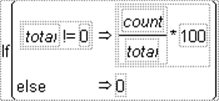
If

Shows a single If condition with a missing expression and a missing then clause. Highlight either expr or then clause and enter a value. For example, to calculate count as a percentage of total when total is not 0, enter the conditional expression (using columns called count and total) in Figure A.3.

Figure A.3 A Conditional Expression

To add a new condition to the If conditional, highlight then clause and click the insert button () on the Formula Editor keypad. Initially, this changes the existing else condition to an expr clause. Click the insert button again to add an else clause. Highlighting then or else and repetitively clicking the insert button changes the else to expr or adds a new expr clause.

To delete a clause, select the then clause above it and press the delete key on your keyboard or click the delete button () on the Formula Editor keypad.

By definition, expressions that evaluate as zero are false. If an expression evaluates as missing, no clauses are executed and missing is returned. All other numeric expressions are true.

Match

Compares an expression to a list of clauses and returns the value of the resulting expression for the first matching clause encountered. You provide the matching expression only once and then give a match value for each clause.

After you select Match in the Formula Editor, a list appears with two options:

•Select Add Match Arguments from Data, and clauses that correspond to all of the levels in your data are added automatically. Alternatively, hold down the SHIFT key, select Conditional, and then select Match. In Figure A.4, the example on the left shows clauses that were added automatically.

•Select Don’t Add so that you can add each clause individually. In Figure A.4, the example on the right shows an empty clause, which you fill with the missing expressions.

Figure A.4 Examples of Using the Match Function

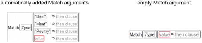
In an automatically filled argument, you should highlight then clause, and then enter an expression. In an empty argument, you highlight either expr, value, or then clause, and then enter an expression. (Or, if you highlight an expression and click Match, the Formula Editor creates a new Match conditional, with the original highlighted expression as expr and nothing for the value and else clause.) Also, keep in mind that:

•Match evaluates faster and uses less memory than an equivalent If because the variable is evaluated only once for each row in the data table. The If condition must evaluate the variable at each If clause for each row until a clause evaluates as true. See “Comparison Functions”, for a comparison of Match and If conditionals.

•With If and Match, the Formula Editor searches down from the top of the sequence for the first true clause and evaluates the corresponding result expression. Subsequent true clauses are ignored.

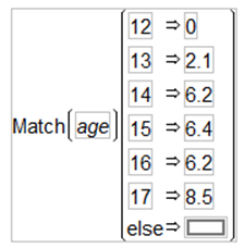
In the following example, each value is assigned depending on the value of the age variable.

Figure A.5 An Example of Using the Match Function

Note: Match ignores trailing spaces and If does not.

Although Match returns missing for any missing values, you can also specifically match missing values.

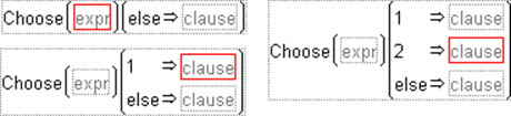
Choose

Choose is a special case of Match in which the arguments of the condition are a sequence of integers starting at one. The value of clause replaces the match condition. An example of a Choose condition is shown in Figure A.6. With Choose, the Formula Editor goes directly to the correct choice clause and evaluates the result expression.

Figure A.6 Example of a Choose Condition

When you highlight an expression and click Choose, the Formula Editor creates a new conditional expression with one clause. Use the insert () and delete () buttons on the keypad to add new clauses or remove unwanted clauses, as described previously for the If conditional.

Choose evaluates the choose expression and goes immediately to the corresponding result expression to generate the returned value. With Choose, you provide a choosing expression that yields sequential integers starting at 1 only once, and then you give a choice for each integer in the sequence.

IfMax

Evaluates the first of each pair of arguments and returns the evaluation of the result expression (the second of each pair) associated with the maximum of the expressions. If more than one expression is the maximum, the first maximum is returned. If all expressions are missing and a final result is not specified, missing is returned. If all expressions are missing and a final result is specified, that final result is returned. The test expressions must evaluate to numeric values, but the result expressions can be anything.

IfMin

Evaluates the first of each pair of arguments and returns the evaluation of the result expression (the second of each pair) associated with the minimum of the expressions. If more than one expression is the minimum, the first minimum is returned. If all expressions are missing and a final result is not specified, missing is returned. If all expressions are missing and a final result is specified, that final result is returned. The test expressions must evaluate to numeric values, but the result expressions can be anything.

And &

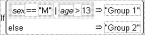
Evaluates as 1 when both of its arguments are true. Otherwise, it evaluates as 0. (See Figure A.9.) The formula in Figure A.7 labels Group 1 as drivers only if both comparisons are true.

Figure A.7 Creating an And Function

Or  |

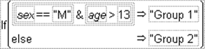
Evaluates as 1 when either of its arguments is true. If both of its arguments are false, then the Or expression evaluates as 0. (See Figure A.9.) The formula in Figure A.8 assigns males and all participants who are more than 13 years old to Group 1.

Figure A.8 Creating an Or Function

The truth tables on the left in Figure A.9 illustrate the results of the And ( & ) and Or (| ) functions when both arguments have nonmissing values that evaluate to true or false. The table on the right illustrates the result when either the left or right expression (call them a and b) or both have missing values.

Figure A.9 Evaluations of And and Or Expressions

Not !

Evaluates as 1 when its argument is false. Otherwise, Not evaluates as 0. When you apply the Not function, use parentheses where necessary to avoid ambiguity. For example, !(weight==64) can be either true or false (either 1 or 0), but (!weight)==64 is always false (0) becauseNot can return only 0 or 1. Expressions such as !(weight==64) can also be entered as weight != 64.

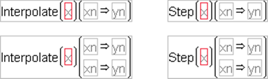
Interpolate

Linearly interpolates the y-value between two points, x1, y1 and x2, y2 that corresponds to the arguments that you give. You can insert additional pairs of x, y arguments with the insert key. Interpolate finds the pair of x, y points that correspond to the x-value and completes the interpolation.

Step

Is like Interpolate except that it returns the y-value corresponding to the greatest x-value less than or equal to the x and y arguments. That is, it finds the corresponding y for a given x from a step function rather than a linear fit between points. Like Interpolate, you can have as many x and yargument pairs as you want.

Figure A.10 Example of Interpolate

For

Repeats the statements in the body argument as long as the while condition is true. The init and next control the iterations.

While

Repeatedly tests the expr condition and executes the body until expr is no longer true.

Break, Continue

Break stops execution of a loop completely and continues to the statement following the loop. Continue ends the current iteration of a loop and begins the loop at the next iteration.

Both are used in For, While, and For Each Row loops.

Stop

Immediately stops a script that is running.

Probability Functions

You can create a formula that calculates probabilities and quantiles for statistical distributions like beta, Chi-square, F, gamma, normal, Student’s t, Weibull distributions, Tukey HSD, and so on. See the Scripting Guide for details about syntax.

Beta Density

Requires three arguments: quantile argument and the shape parameters alpha and beta. A threshold parameter (θ) and a scale parameter (σ > 0) are additional arguments. It returns the value of the beta probability density function (pdf) for the given arguments. The beta density is useful for modeling the probabilistic behavior of random variables such as proportions constrained to fall in the interval [0, 1].

Beta Distribution

The beta distribution has two shape parameters: α > 0 and β > 0. A threshold parameter (θ) and a scale parameter (σ) are additional arguments, where θ≤ x ≤θ + σ. The default value for θ is 0. The default value for σ is 1.

The beta distribution function is the inverse of the beta quantile function.

Beta Quantile

Accepts a probability argument, p, and shape and scale parameters, α > 0 and β > 0. It returns the p^th quantile from the standard beta distribution. The beta quantile function is the inverse of the beta distribution function.

ChiSquare Density

Accepts a quantile argument from the range of values for the Chi-squared distribution, a degrees of freedom argument, and an optional noncentrality parameter. It returns the value of the Chi-squared density function (pdf) for the arguments.

ChiSquare Distribution

Accepts a response argument (range of x values) and three parameter arguments: a quantile, a degrees of freedom, and a noncentrality parameter. It returns the probability that an observation from the Chi-squared distribution with the specified noncentrality parameter and degrees of freedom is less than or equal to the given quantile. For example, the expression ChiSquare Distribution(11.264, 5) returns the probability that an observation from the Chi-squared distribution centered at 0 with 5 degrees of freedom is less than or equal to 11.264. The expression evaluates as 0.95361.

Furthermore, the ChiSquare Distribution function accepts integer and noninteger degrees of freedom. It is centered at 0 by default. The ChiSquare Distribution function is the inverse of the ChiSquare Quantile function.

ChiSquare Quantile

Accepts three arguments: a probability p, a degrees of freedom, and a noncentrality parameter. It returns the p^th quantile from the Chi-squared distribution with the specified noncentrality parameter and degrees of freedom. For example, the expression ChiSquare Quantile(.95, 3.5, 4.5)returns the 95% quantile from the Chi-squared distribution centered at 4.5 with 3.5 degrees of freedom. The expression evaluates as 17.50458.

The ChiSquare Quantile function accepts integer and noninteger degrees of freedom. It is centered at 0 by default. The ChiSquare Quantile function is the inverse of the ChiSquare Distribution function.

Dunnett P Value

Returns the p-value from Dunnett’s multiple comparison test.

Dunnett Quantile

Returns the quantile needed in Dunnett’s multiple comparison tests.

F Density

Accepts a quantile argument from the range of values for the F-distribution, numerator and denominator degrees of freedom arguments, and an optional noncentrality parameter. It returns the value of the F-density function (pdf) for the arguments.

F Distribution

Accepts four arguments: a quantile, a numerator and denominator degrees of freedom, and a noncentrality parameter. It returns the probability that an observation from the F-distribution with the specified noncentrality parameter and degrees of freedom is less than or equal to the given quantile. For example, the expression F Distribution(3.32, 2, 3) returns the probability that an observation from the central F-distribution with 2 degrees of freedom in the numerator and 3 degrees of freedom in the denominator is less than or equal to 3.32. The expression evaluates as 0.82639.

The F-distribution function accepts integer and noninteger degrees of freedom. By default, the non-central parameter is set to 0. The F-distribution function is the inverse of the F Quantile function.

F Quantile

Accepts four arguments: a probability p, a numerator and denominator degrees of freedom, and a noncentrality parameter. It returns the p^th quantile from the F-distribution with the specified noncentrality parameter and degrees of freedom. For example, the expression F Quantile(0.95, 2, 10, 0) returns the 95% quantile from the F-distribution centered at 0 with 2 degrees of freedom in the numerator and 10 degrees of freedom in the denominator. The expression evaluates as 4.1028.

The F Quantile function accepts integer and noninteger degrees of freedom. By default, the non-central parameter is set to 0. The F Quantile function is the inverse of the F Distribution function.

Frechet Density

Returns the density at x of a Fréchet distribution with location mu and scale sigma.

Frechet Distribution

Returns the probability that a Fréchet distribution with location mu and scale sigma is less than x.

Frechet Quantile

Returns the quantile associated with a cumulative probability p for a Fréchet distribution with location mu and scale sigma.

Gamma Density

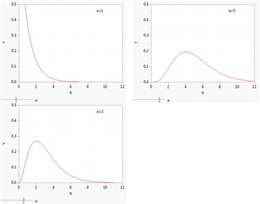
Requires a quantile argument. Also accepts an optional alpha shape parameter, which must be greater than zero and defaults to 1. A scale parameter b, which must be greater than zero and defaults to 1, is optional. A threshold parameter, which must be in the range -∞ < θ < +∞ and defaults to zero, is optional.

Figure A.11 shows the shape of gamma probability density functions for shape parameters of 1, 3, and 5. The standard gamma density function is strictly decreasing when α (shape) ≤1. When α > 1 the density function begins at zero when x is θ, increases to a maximum, and then decreases.

Figure A.11 Gamma Density Example

Gamma Distribution

Is based on the standard gamma function, and accepts a single argument with a quantile value. The shape, scale, and threshold parameters are optional, with defaults as described previously in the discussion of the Gamma Density function. It returns the probability that an observation from a standard gamma distribution is less than or equal to the specified x. The Gamma Distribution function is the inverse of Gamma Quantile function.

Gamma Quantile

Accepts a probability argument p, and returns the p^th quantile from the standard gamma distribution with the shape parameter that you specify. The Gamma Quantile function is the inverse of the Gamma Distribution function.

LEV Density

Returns the density at x of the largest extreme value distribution with location mu and scale sigma.

LEV Distribution

Returns the probability that the largest extreme value distribution with location mu and scale sigma is less than x.

LEV Quantile

Returns the quantile associated with a cumulative probability p of the largest extreme value distribution with location mu and scale sigma.

Logistic Density

Returns the density at x of a logistic distribution with location mu and scale sigma.

Logistic Distribution

Returns the probability that the logistic distribution with location mu and scale sigma is less than x.

Logistic Quantile

Returns the quantile associated with a cumulative probability p of the logistic distribution with location mu and scale sigma.

Loglogistic Density

Returns the density at x of the loglogistic distribution with location mu and scale sigma.

Loglogistic Distribution

Returns the probability that the loglogistic distribution with location mu and scale sigma is less than x.

Loglogistic Quantile

Returns the quantile associated with a cumulative probability p of the loglogistic distribution with location mu and scale sigma.

Lognormal Density

Returns the density at x of the lognormal distribution with location mu and scale sigma.

Lognormal Distribution

Returns the probability that the lognormal distribution with location mu and scale sigma is less than x.

Lognormal Quantile

Returns the quantile associated with a cumulative probability p of a lognormal distribution with location mu and scale sigma.

Normal Density

Accepts an argument from the range of values for the standard normal distribution, which is all real numbers. It returns the value of the standard normal probability density function (pdf) for the argument. For example, you can create a column of values (X) with the formula count(-3, 3, nrow()). In a second column, insert the formula Normal Density(X) to generate density values. Then select Graph > Graph Builder to plot the normal density by X.

Normal Distribution

Accepts an argument x from the range of values for the standard normal distribution, which is all real numbers. It returns the probability that an observation from the standard normal distribution is less than or equal to x. For example, the expression Normal Distribution(1.96) returns 0.975, the probability that an observation from the standard normal distribution is less than or equal to the 1.96^th quantile. Also, you can specify mean and standard deviation parameters to obtain probabilities from nonstandard normal distributions. The Normal Distribution function is the inverse of the Normal Quantile function.

Normal Quantile (Probit)

Accepts a probability argument p, and returns the p^th quantile from the standard normal distribution. For example, the expression Normal Quantile(0.975) returns the 97.5% quantile from the standard normal distribution, which evaluates as 1.96. Also, you can specify parameter values for the mean and standard deviation to obtain quantiles from nonstandard normal distributions. The Normal Quantile function is the inverse of the Normal Distribution function.

Normal Biv Distribution

Computes the probability that an observation is less than or equal to (x,y) with correlation coefficient r where the observation is marginally normally distributed. You can specify the mean and standard deviation for the X and Y coordinates of the observation. The default values are 0 for both means and 1 for both standard deviations.

GLog Density

Returns the density or pdf at a particular quantile q of a generalized logarithm distribution with location mu, scale sigma, and shape lambda. When the shape parameter is equal to zero, the distribution reduces to a Lognormal(mu, sigma).

GLog Distribution

Returns the probability or cdf that a generalized logarithm distributed random variable is less than q. When the shape parameter is equal to zero, the distribution reduces to a Lognormal(mu, sigma).

GLog Quantile

Returns the quantile, the value for which the probability is p that a random value would be lower. When the shape parameter is equal to zero, the distribution reduces to a Lognormal(mu, sigma).

SEV Density

Returns the density at x of the smallest extreme distribution with location mu and scale sigma.

SEV Distribution

Returns the probability that the smallest extreme distribution with location mu and scale sigma is less than x.

SEV Quantile

Returns the quantile associated with a cumulative probability p of the smallest extreme distribution with location mu and scale sigma.

t Density

Accepts a quantile argument from the range of values for the t-distribution, a degrees of freedom argument, and an optional noncentrality parameter. It returns the value of the t-density function (pdf) for the arguments. To compare a t-density with 5 df with a standard normal distribution, you can create a column of quantile values (X) with the formula count(-3, 3, nrow()). In a second column, insert the formula t Density(X). In a third column, insert the formula Normal Density(X). Then select Graph > Graph Builder to plot the t-density and the normal density by X. You will see that the t-density has slightly more spread than the normal.

t Distribution

Accepts three arguments: a quantile, a degrees of freedom, and a noncentrality parameter. It returns the probability that an observation from the Student’s t-distribution with the specified noncentrality parameter and degrees of freedom is less than or equal to the given quantile. For example, the expression t Distribution(.9, 5) returns the probability that an observation from the Student’s t-distribution centered at 0 with 5 degrees of freedom is less than or equal to 0.9. The expression is evaluated as 0.79531. t-distribution accepts integer and noninteger degrees of freedom. It is centered at 0 by default, but you can enter a value for the noncentrality parameter. The t Quantile function is the inverse of the t Distribution function.

t Quantile

Accepts three arguments: a probability p, a degrees of freedom, and a noncentrality parameter. It returns the p^th quantile from the Student’s t-distribution with the specified noncentrality parameter and degrees of freedom. For example, the expression Student’s t Quantile(.95, 2.5) returns the 95% quantile from the Student’s t-distribution centered at 0 with 2.5 degrees of freedom. The expression evaluates as 2.558219. The t Quantile function is the inverse of the t Distribution function. This function also accepts integer and noninteger degrees of freedom. It is centered at 0 by default, but you have the option to enter a value for the noncentrality parameter. The t Distribution function is the inverse of the t Quantile function.

Weibull Density

Accepts a quantile argument from the range of values for the Weibull distribution, and optional shape, scale, and threshold arguments. The density function for a Weibull distribution with shape parameter β, scale parameter α, and threshold parameter θ is given in the Basic Analysis book. The Weibull Density function returns the value of the probability density function (pdf) for the corresponding Weibull distribution.

Weibull Distribution

Accepts a quantile argument x from the range of values for the Weibull distribution, and optional shape, scale, and threshold arguments. The density function for a Weibull distribution with shape parameter β, scale parameter α, and threshold parameter θ is given in the Basic Analysis book. The Weibull Distribution function returns the probability that an observation is less than or equal to the specified x for the Weibull distribution with the shape, scale, and threshold parameters that you specified. The Weibull Distribution function is the inverse of Weibull Quantilefunction.

The Weibull distribution has different shapes depending on the values of α (a scale parameter that affects the x direction) and β (a shape parameter). It often provides a good model for estimating the length of life, especially for mechanical devices and in biology. The two-parameter Weibull is the same as the three-parameter Weibull with a threshold of zero.

Weibull Quantile

Accepts a probability argument p, and returns the p^th quantile from the Weibull distribution with the shape, scale, and threshold parameters that you specify. The Weibull Quantile function is the inverse of the Weibull Distribution function.

Cauchy Density

Accepts an argument x, which can be any real number, and optional arguments center and scale. If you do not specify values for the optional arguments, the function returns the value at x of the Cauchy probability density function (pdf) for a distribution with median 0 and third quartile 1.

If you specify values for center and scale, the function returns the value at x of the Cauchy probability function, characterized as follows:

•The optional parameter center is the median of the distribution.

•The optional parameter scale is half of the interquartile range, namely, half of the difference between the 0.75 and 0.25 quantiles.

Cauchy Distribution

Accepts an argument x, which can be any real number, and optional arguments center and scale. If you do not specify values for the optional arguments, the function returns the value at x of the Cauchy cumulative distribution function (cdf) for a distribution with median 0 and third quartile 1. If you specify values for center and scale, the function returns the value at x of the cumulative distribution function for the Cauchy distribution with median given by center and interquartile range given by twice the scale.

Cauchy Quantile

Accepts an argument prob, which can be any number between 0 and 1, and optional arguments center and scale. If you do not specify values for the optional arguments, the function returns the p^th quantile, where p = prob, of a Cauchy distribution with median 0 and third quartile 1. If you specify values for center and scale, the function returns the p^th quantile of a Cauchy distribution with median given by center and interquartile range given by twice the scale.

Johnson Su Distribution

Returns the probability that a Johnson Su-distributed random variable is less than x. There are four optional arguments: gamma, delta, theta, and sigma. For a description of the Johnson Su distribution and these parameters, see the Basic Analysis book.

Johnson Su Quantile

Returns the p^th quantile of the Johnson Su distribution. There are four optional arguments: gamma, delta, theta, and sigma. For a description of the Johnson Su distribution and these parameters, see the Basic Analysis book.

Johnson Su Density

Returns the density at x of a Johnson Su distribution. There are four optional arguments: gamma, delta, theta, and sigma. For a description of the Johnson Su distribution and these parameters, see the Basic Analysis book.

Johnson Sb Distribution

Returns the probability that a Johnson Sb-distributed random variable is less than x. There are four optional arguments: gamma, delta, theta, and sigma. For a description of the Johnson Sb distribution and these parameters, see the Basic Analysis book.

Johnson Sb Quantile

Returns the p^th quantile of the Johnson Sb distribution. There are four optional arguments: gamma, delta, theta, and sigma. For a description of the Johnson Sb distribution and these parameters, see the Basic Analysis book.

Johnson Sb Density

Returns the density at x of a Johnson Sb distribution. There are four optional arguments: gamma, delta, theta, and sigma. For a description of the Johnson Sb distribution and these parameters, see the Basic Analysis book.

Johnson Sl Distribution

Returns the probability that a Johnson Sl-distributed random variable is less than x. There are four optional arguments: gamma, delta, theta, and sigma. For a description of the Johnson Sl distribution and these parameters, see the Basic Analysis book.

Johnson Sl Quantile

Returns the p^th quantile of the Johnson Sl distribution. There are four optional arguments: gamma, delta, theta, and sigma. For a description of the Johnson Sl distribution and these parameters, see the Basic Analysis book.

Johnson Sl Density

Returns the density at x of a Johnson Sl distribution. There are four optional arguments: gamma, delta, theta, and sigma. For a description of the Johnson Sl distribution and these parameters, see the Basic Analysis book.

Tukey HSD Quantile

Accepts a probability argument 1-alpha, and returns the 1-alphath quantile from Tukey’s HSD test for the parameters that you specify. The alpha argument is the significance level that you want. nGroups is the number of groups in a study. dfe is the error degrees of freedom (based on the total study sample). This is the quantile used to calculate least significant difference in Tukey’s multiple comparisons test.

Tukey HSD P Quantile

Returns the p-value from Tukey's HSD multiple comparisons test.

F Power and F Sample Size

The F Power function calculates the power from a given situation that involves an F-test or t-test, and the F Sample Size function computes the sample size. The arguments are the values that you specify for computation of a prospective power analysis. (These functions perform the same computations as if you selected DOE > Sample Size and Power. See the Design of Experiments Guide for a discussion of power and sample size.) The arguments include:

•alpha The significance level that you are willing to tolerate (often 0.05).

•dfh The hypothesis degrees of freedom. It is one (1) for a t-test.

•dfm The model degrees of freedom (such that dfe = n – dfm).

•SquaredSize The squared effect size scaled by the error variance, which is used for making the noncentrality argument for the F-distribution. For this argument, use squared size = Δ²/σ² where σ² is the error variance. That is, use:

for a one-sample t-test

for a two-sample t-test

for a k-sample F-test

•n (found only in the F Power function) The total number of observations (runs, experimental units, or samples) you expect to have. Power (in the F Sample Size function) is the probability that you want to have of declaring a significant result.

Discrete Probability Functions

Gamma Poisson Probability

Returns the probability or pmf that a gamma-Poisson distributed random variable is equal to x. In general, the gamma Poisson functions accept arguments that are the mean parameter lambda, the overdispersion parameter sigma, and the count of interest x. When the overdispersion is equal to one, the Gamma Poisson reduces to a Poisson(lambda) distribution.

Gamma Poisson Distribution

Returns the probability that a gamma-Poisson distributed random variable is less than or equal to x. In general, the gamma Poisson functions accept arguments that are the mean parameter lambda, the overdispersion parameter sigma, and the count of interest x.

Gamma Poisson Quantile

Returns the smallest integer quantile for which the cumulative probability of the Gamma Poisson (lambda, sigma) distribution is larger than or equal to p.

Binomial Distribution

Returns the probability that an observation from a binomial distribution with parameters p and n is less than or equal to k. In general, the binomial functions accept arguments that are the probability of success p (the event of interest), the number of trials n, and the number of successes k.

Binomial Probability

Computes the probability that a random variable from a binomial distribution is equal to k. In general, the binomial functions accept arguments that are the probability of success p (the event of interest), the number of trials n, and the number of successes k.

Binomial Quantile

Returns the smallest integer quantile for which the cumulative probability of the Binomial (p, n) distribution is larger than or equal to the specified probability.

Neg Binomial Distribution

Returns the probability that a negative binomially distributed random variable is less than or equal to k, where the probability of success is p, and the number of successes is n.

Neg Binomial Probability

Returns the probability that a negative binomially distributed random variable is equal to k, where the probability of success is p, and the number of successes is n.

Beta Binomial Distribution

Returns the probability or pmf that a beta binomially distributed random variable is less than or equal to x. In general, the beta binomial functions accept arguments that are the probability of success p (the event of interest), the overdispersion parameter delta, and the number of trials n. When the overdispersion parameter for the beta binomial is zero, the distribution reduces to a binomial(p, n).

Beta Binomial Probability

Returns the probability or cmf that a beta binomially distributed random variable is equal to x. When the overdispersion parameter for the beta binomial is zero, the distribution reduces to a binomial(p, n).

Beta Binomial Quantile

Returns the smallest integer quantile for which the cumulative probability of the Beta Binomial (p, n, delta) distribution is larger than or equal to the specified probability. When the overdispersion parameter for the beta binomial is zero, the distribution reduces to a binomial (p, n).

Hypergeometric Distribution

Computes the probability that a random variable from a hypergeometric distribution is less than or equal to x. The hypergeometric distribution models the total number of successes in a fixed sample drawn without replacement from a finite population. The hypergeometric functions accept as arguments the size of the population N, the total number of items with the desired characteristic in the population, K, the number of samples drawn n, and the number of successes in the sample x.

Hypergeometric Probability

Computes the probability that a random variable from a hypergeometric distribution is equal to x.

Poisson Distribution

Computes the probability that a random variable from a Poisson distribution with mean lambda is less than or equal to the count of interest. In general, Poisson functions accept an argument that is the count of interest, and lambda, the mean parameter.

Poisson Probability

Computes the probability that a random variable from a Poisson distribution with mean lambda is equal to the count of interest.

Poisson Quantile

Returns the smallest integer quantile for which the cumulative probability of the Poisson (lambda) distribution is larger than or equal to p.

Statistical Functions

There are two types of Statistical functions you can use in a formula:

•The functions with names that have the prefix Col. These functions compute statistics for a column of numbers or expressions involving columns.

•The Mean, Std Dev, Number, Sum, Quantile, Maximum, Minimum, and N Missing functions. These functions evaluate across columns or arguments. The statistic is computed for each row across the series of arguments. You can use the insert key on the on-screen keypad, or type a comma to add arguments to the functions that accept multiple arguments. When there are multiple contiguous arguments, select the function and the first argument, and then Shift-click the last argument in the group. These functions then automatically show with the complete list.

See the Scripting Guide for details about syntax.

Col Mean

Calculates the mean (or arithmetic average) of the numeric values identified by its argument. The formula Col Mean(age) calculates the average of all nonmissing values in the age column.

Col Std Dev

Measures the spread around the mean of the distribution identified by its argument. In the normal distribution, about 68% of the distribution is within one standard deviation of the mean. 95% of the distribution is within two standard deviations of the mean. 99% of the distribution is within three standard deviations of the mean.

Col Number

Counts the number of nonmissing values in the column that you specify. A missing numeric value occurs when a cell has no assigned value or is the result of an invalid operation (such as division by zero). Missing values show on the spreadsheet as a missing value mark (•). Missing character values are null character strings. In formulas for row state columns, an excluded row state characteristic is treated as a missing value.

Col N Missing

Counts the number of missing values in the column that you specify. A missing numeric value occurs when a cell has no assigned value or is the result of an invalid operation (such as division by zero). Missing values show in the data grid with a missing value character (•). Missing character values are null character strings.

Col Sum

Computes the sum of the values in its numeric argument. Missing values are ignored.

Col Minimum and Col Maximum

Takes the minimum of its numeric arguments. Col Minimum ignores missing values. Col Maximum takes the maximum of a numeric column argument and ignores missing values.

Col Quantile

Computes the value at which a specific percentage of the values is less than or equal to that value. For example, the value calculated as the 50% quantile, also called the median, is greater than or equal to 50% of the data. Half of the data values are less than the 50^th quantile.

The Col Quantile function’s quantile argument represents the quantile percentage divided by 100. The 25% quantile, also called the lower quartile, corresponds to p = 0.25, and the 75% quantile, called the upper quartile, corresponds to p = 0.75.

The Formula Editor computes a quantile for a column of n nonmissing values by arranging the values in ascending order. The subscripts of the sorted column values, y₁, y₂,...,y_n, represent the ranks in ascending order.

The pth quantile value is calculated using the formula p(n + 1), where p is the percent value and n is the total number of nonmissing values. If p(n+1) is an integer, then the quantile value is y_p(n₊₁₎. If p(n + 1) is not an integer, then the value is interpolated by assigning the integer part of the result to i, assigning the fractional part to f, and applying the formula (1 – f)y_i + (f)y_i+1.

For example, suppose a column has values 2, 4, 6, 8, 10, 12, 14, 16, 18, and 20. The 50% quantile is calculated as 0.5(10 + 1) = 5.5.

Because the result is fractional, the 50% quantile value is interpolated as

(1 – 0.5) x 10 + (0.5) x 12 = (0.5)10 + (0.5)12 = 6 + 5 = 11

The following are example ColQuantile formulas:

•ColQuantile(age, 1) Calculates the maximum age.

•ColQuantile(age, 0.75) Calculates the upper quartile age.

•ColQuantile(age, 0.5)  Calculates the median age.

•ColQuantile(age, 0.25) Calculates the lower quartile age.

•ColQuantile(age, 0) Calculates the minimum age.

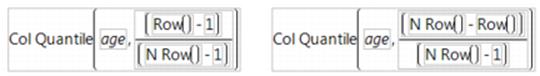
The ColQuantile argument can be any expression that evaluates to a value between (and including) 0 and 1. For example, the first formula in Figure A.12 calculates quantile values of age in ascending order for each row. The column then contains the interpolated values of age in ascending order in the calculated column. The second formula lists the interpolated values of age in descending order.

Figure A.12 Examples of the Quantile Function

Col Rank

Ranks each row’s value, from 1 for the lowest value to the number of non-missing columns for the highest value. Ties are broken arbitrarily.

Col Standardize

Performs the usual standardization on its numeric expression. For each row i, Col Standardize(height) is (HeightRow()–Col Mean(Height))/Col Std Dev(Height).

Mean

Calculates the arithmetic average of the nonmissing arguments that you specify. The arguments can be constants, numbers, or expressions. The Mean function initially shows with a single argument. You add arguments with the insert button () on the Formula Editor keypad or by typing a comma.

Std Dev

Computes standard deviation of the list of arguments that you specify. The arguments can be constants, numbers, or expressions. The Std Dev function initially shows with a single argument. You add arguments by clicking the insert button () on the Formula Editor keypad or by typing a comma.

Number

Counts the number of nonmissing values in the list of arguments that you specify.

Sum

Returns the sum of the arguments.

Quantile

Calculates the quantile given by its first argument for all the following arguments given.

Summation (Σ)

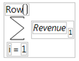
Evaluates for an explicit range of values in a column, as given by the summation indices. This behavior is different from all other statistical functions (except Product), which always evaluate on every row. The Summation function uses the summation notation shown in Figure A.13. To calculate a sum, replace the missing body term with an expression containing the index variable i, or an index variable that you assign. Summation repeatedly evaluates the expression for i = 1, i = 2, through i = NRow() and then adds the nonmissing results together to determine the final result.

You can replace NRow(), the number of rows in the active spreadsheet, and the index constant, i, with any expression appropriate for your formula. For example, the summation formula in Figure A.13 computes the total for each row of all revenue values for rows 1 through the current row number, filling the calculated column with the cumulative totals of the revenue column.

Figure A.13 Example of the Summation function

Product (Π)

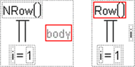
Evaluates for an explicit range of values in a column, as given by the summation indices, as opposed to all other statistical functions (except Summation), which always evaluate on every row. Product uses the notation shown in the formulas on the right in Figure A.14. To calculate a product, replace the missing body term with an expression containing the index variable j. Product repeatedly evaluates the expression for i = 1, i = 2, through i = n and multiplies the nonmissing results together to determine the final result.

You can replace NRow(), the number of rows in the active spreadsheet and the index constant, i, with any expression appropriate for your formula.

For example, the expression second product example in Figure A.14 calculates i! (each row number’s factorial).

Figure A.14 Examples of the Product Function

Minimum and Maximum

Return the minimum and maximum value, respectively, from the list of nonmissing arguments that you specify.

N Missing

Counts the number of missing values in the list of arguments that you specify.

Desirability

Are smooth piecewise functions that are crafted to fit the control points. The minimize and maximize functions are three-part piecewise smooth functions that have exponential tails and a cubic middle.

The target function is a piecewise function. It is a scale multiple of a normal density on either side of the target (with different curves on each side), which is also piecewise smooth and fit to the control points.

Random Functions

You can create formulas that generate real numbers by effectively “rolling the dice” within the constraints of the specified distribution. Each time you click Apply in the Formula Editor window, these functions produce a new set of random numbers.

Note: Random numbers are generated using the Mersenne-Twister technique. This technique has a period length of 2¹⁹⁹³⁷-1. For details about the generators, see Matsumoto and Nishimura (1998). The new generators are verified to pass all the DIEHARD tests as documented in Marshalled (1996).

See the Scripting Guide for details about syntax.

Random Uniform

Generates random numbers uniformly between 0 and 1. This means that any number between 0 and 1 is as likely to be generated as any other. The result is an approximately even distribution. You can shift the distribution and change its range with constants. For example,5 + Random Uniform()*20 generates uniform random numbers between 5 and 25.

Random Normal

Generates random numbers that approximate a normal distribution with a mean of 0 and standard deviation of 1 if no arguments are used, or with the mean and standard deviation entered as arguments. The normal distribution is bell shaped and symmetrical. You can also modify the Random Normal function with constants if no arguments are entered to give a normal distribution with specific mean and standard deviation. For example, the formula Random Normal()*5 + 30 generates a random normal variable with a mean of 30 and a standard deviation of 5.

Random Exp

Generates a single parameter exponential distribution for the distribution parameter lambda=1. You can modify the exponential function to use a different lambda.

For example, Random Exp()/.1 generates an exponential distribution for lambda=0.1. The exponential distribution is often used to model simple failure time data, where lambda is the failure rate.

Random Gamma

Gives a gamma distribution for the parameter, alpha, you enter as the function argument. The gamma distribution describes the time until the k^th occurrence of an event. The gamma distribution can also have a scale parameter, beta. A gamma variate with shape parameter alpha and scale beta can be generated with the formula beta*Random Gamma(alpha). If 2*alpha is an integer, a Chi-squared variate with 2*alpha degrees of freedom is generated with the formula 2*Random Gamma(alpha).

Random Beta

Generates a pseudo-random number distributed Beta(alpha, beta).

Random Cauchy

Generates a Cauchy distribution with location parameter 0 and scale parameter 1. The Cauchy distribution is bell shaped and symmetric but has heavier tails than the normal distribution. A Cauchy variate with location parameter alpha and scale parameter beta can be generated with the formula alpha+beta*Random Cauchy().

Random Category

Generates a random category given an alternation of probability and result expressions (for example, Random Category(.2, "A", .3, "B", .4, "C", "D");).

Random Johnson Su

Returns a random number from the Johnson Su distribution.

Random Johnson Sb

Returns a random number from the Johnson Sb distribution.

Random Johnson Sl

Returns a random number from the Johnson Sl distribution.

Random Triangular

Generates a triangular distribution of numbers between 0 and 1, with the midpoint that you enter as the function argument. You can add a constant to the function to shift the distribution and multiply to change its span.

Random Integer

Generates a uniform distribution of integers between 1 and the argument that you enter as n1, if nothing is entered for n2. If you enter both n1 and n2 (n1<n2), Random Integer generates a uniform distribution of the integers between and including n1 and n2.

Random Binomial

Generates random numbers from a binomial distribution with parameters that you enter as function arguments. The first argument is n, the number of trials in a binomial experiment. The second argument is p, the probability that the event of interest occurs. When n is 1, the binomial function generates a distribution of Bernoulli trials. For example, n =1 and p = 0.5, give the distribution of tossing a fair coin. The mean of the binomial distribution is np, and variance is np(1 – p).

Random Negative Binomial

Generates a negative binomial distribution for the parameters that you enter as function arguments. The first parameter is the number of successes of interest (r) and the second argument is the probability of success (p). The random variable of interest is the number of failures that precede ther^th success. In contrast to the binomial variate, where the number of trials is fixed and the number of successes is variable, the negative binomial variate is for a fixed number of successes and a random number of trials. The mean of the negative binomial distribution is (r(1 – p))/p and the variance is (r(1 – p))/p².

Random Beta Binomial

Returns random numbers from the beta binomial distribution for n trials with probability p and correlation or overdispersion delta.

Random Frechet

Returns a random number from a Fréchet distribution with the location mu and scale sigma.

Random Geometric

Returns random numbers from the geometric distribution with the parameter that you enter as the function argument. The parameter, p, is the probability that a specific event occurs at any one trial. The number of trials until a specific event occurs for the first time is described by the geometric distribution. The mean of the geometric distribution is (1-p)/p, and the variance is (1 – p)/p².

Random Poisson

Generates a Poisson variate based on the value of the parameter, lambda, you enter as the function argument. Lambda is often the expected number of events occurring per unit time or unit of area. Lambda is both the mean and the variance of the Poisson distribution.

Random Gamma Poisson

Returns random numbers from the gamma Poisson distribution with parameters lambda and sigma.

Random Weibull

Returns a random number from a Weibull distribution.

Random Logistic

Returns a random number from a logistic distribution with the location mu and scale sigma.

Random Loglogistic

Returns a random number from a loglogistic distribution with the location mu and scale sigma.

Random Lognormal

Returns a Lognormal-distributed random number with location parameter mu and scale sigma.

Random GLog

Returns random numbers from the generalized logarithm distribution with parameters mu, sigma, and lambda. When lambda is equal to zero, the function returns a lognormal(mu, sigma).

Random Reset

Restarts the random number sequences with a seed that you specify.

Random LEV

Returns a random number from an LEV distribution with the specified location mu and scale sigma.

Random SEV

Returns a random number from the smallest extreme distribution with the specified location mu and scale sigma.

Col Shuffle

Selects a row number at random from the current data table. Each row number is selected only once. When Col Shuffle is used as a subscript, it returns a value selected at random from the column that serves as its argument. Each value from the original column is assigned only once as Col Shuffle’s result.

For example, to identify a 50% random sample without replacement, use the formula in Figure A.15.

Figure A.15 Formula Identifying 50% Random Sample

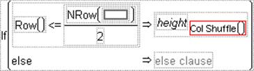
The formula in Figure A.15 selects half the values (n/2) from the column x and assigns them to the first half of the rows in the computed column. The remaining rows of the computed column fill with missing values.

Resample Freq

Generates a random selection with replacement frequency counts, suitable for use in bootstrapping. For example, it supports a second Freq Column argument, enabling it to do bootstrap samples relating to a pre-existing frequency column specified in the second argument. Resample Freq() generates a 100% resample. ResampleFreq(rate) generates a rate frequency sample. Resample(rate, column) generates a sample that is calculated by the rate multiplied by the sum of the specified column.

Date Time Functions

JMP stores dates and times in numeric columns using the Macintosh standard of the number of seconds since January 1, 1904. When a column has date values, you can assign a date format to that column by double-clicking a column name and selecting Date or Time from the Formatmenu. See “Numeric Format Options” in the “The Column Info Window” chapter.

See the Scripting Guide for details about syntax.

In Minutes, In Hours, In Days, In Weeks, In Years

Converts from the units of the function name to the equivalent number of seconds for the argument. The argument must be a number or numeric expression. For example, In Minutes(2) yields 120, and In Years(1) yields 31,557,600 (60 seconds * 60 minutes * 24 hours * 365.25 days).

Date DMY, Date MDY

Accepts numeric expressions for day, month, and year and return the associated JMP date. For example, Date DMY (20, 3, 1991) and Date MDY(3, 20, 1991) evaluate to 2,752,272,000.

Today

Returns the number of seconds between January 1, 1904 and the current date. For example, at midnight on March 20, 1991 (a Wednesday), the Today function returns 2752272000 (2,752,272,000 seconds) and continues counting. If you evaluate the Today function later in the day, it reflects the additional seconds.

Day, Month, Year,

Returns the day of the month, the month (as a number from 1 to 12), a four-digit year, respectively. The argument for these functions is interpreted as a JMP date. For example, on March 20, 1991:

•Day(2752272000) returns the number 20.

•Month(2752272000) returns the number 3.

•Year(2752272000) returns the number 1991.

Quarter

Returns the annual quarter of a datetime value as an integer 1-4.

Hour, Minute, Second

Returns the hour, the minute, and the seconds of a date-time value, respectively. The argument for these functions is interpreted as a JMP date. For example, on March 20, 1991:

•Hour(2752572649) returns the number 11.

•Minute(2752572649) returns the number 30.

•Second(2752572649) returns the number 49.

Day of Week, Day of Year, Week of Year, Time of Day

The argument for these functions is a JMP date. Day Of Week returns a number from 1 to 7, where 1 represents Sunday. Day Of Year returns the number of days from the beginning of the year. Week Of Year returns a number from 1 to 52 based on the rule specified. Rule 1 (default) has weeks start on Sunday with the first Sunday being week 2 and week 1 is a partial week or empty; rule 2 has the first Sunday begins week 1 with any previous days being week 0; rule 3 returns the ISO week number where the week starts on Monday and week 1 is the first week of the year with four days in that year. With ISO weeks, it is possible for the first or last three days of the year to belong to the neighboring year’s week number. Time Of Day returns a number from 0 to 86399 (time of day in seconds). For example, on Wednesday, March 20, 1991:

•Day Of Week(2752272000) returns the number 4.

•Day Of Year(2752272000) returns the number 79.

•Week Of Year(2752272000) returns the number 12.

•Time Of Day(2752272000) returns the number 0.

Informat

The argument for the Informat function is a date character string. For example, Informat("03/20/1991") returns the appropriate JMP date value, 2752272000. JMP can read all the date formats except for Abbrev Date and Long Date.

Abbrev Date, Long Date, Short Date

The argument for these date functions is a JMP date. They return character strings that are the formatted representation of the argument. For example:

•Abbrev Date(2752272000) returns Wed, Mar 20,1991.

•Long Date(2752272000) returns Wednesday, March 20, 1991.

•Short Date(2752272000) returns 3/20/91.

Format

The first argument in the Format function is a JMP date. This function returns the character string representation of the date by the date format that you specify in the second argument, which is a quoted string. If you apply this formula to a numeric column, JMP automatically changes the column’s data type to character.

You can also supply a column for the first argument and leave the rest blank. The result is the formatted value of the column reference. This can be used to extract value labels of a column when the value labels are turned off.

MDYHMS

The argument of MDYHMS is a JMP date. This function shows all date and time fields, appending zeros as time fields if no time information is present. This is useful if a date column is formulated such that not all date information is displayed. The MDYHMS function can be used to see all available date and time information.

Date Increment

Adds 1 or more intervals to a starting datetime value. For example, Date Increment(Today(), "Day", 3) adds three days to the current date. Date Increment(Today(), "Year", 3) adds 3 years to the current date.

Date Difference

Returns the difference of two datetime values. The interval argument can be Second, Minute, Hour, Day, Week, Month, Quarter, Year. The alignment arguments are described here:

Start

is used to count the number of times an interval starts.

Actual

is used to count whole intervals.

Fractional

is used to count fractional intervals.

For example, the following formula returns 207.890243055556, the number of days between the dates:

Date Difference(01Jan2010:00:00:00, 27Jul2010:21:21:57, "Day", "fractional");

The following formula returns 207, the number of completed days between the dates:

Date Difference(01Jan2010:00:00:00, 27Jul2010:21:21:57, "Day", "actual");

The following formula returns 9, the number of completed hours between the times:

Date Difference(01Jan2010:00:00:00, 01Jan2010:09:22:57, "Hour", "actual");

The following formula returns 1, the number of times a new hour started between the times:

Date Difference(31Dec2010:23:59:59, 01Jan2011:00:59:59, "Hour", "start");

Row State Functions

There are six characteristics that rows in a data table can have: selected, hidden, excluded, labeled, colored, and marked. If you give rows one or more of these characteristics and then create row state data table columns, you can then create a formula that computes and saves row state conditions. (See “Column Properties” in the “The Column Info Window” chapter, and “Row State Columns” in the “The Column Info Window” chapter.)This formula processes row state data just as it would process character and numeric data.

See the Scripting Guide for details about syntax.

Note: A row can be assigned any combination of row states; a row state column can have multiple row states as a value.

Table A.2 describes the type of argument each Row State function requires and what each returns.

Row State

Returns the active row state condition of the current row as true or false. You can use this function to conveniently write conditional clauses that depend on the status of the current row. For example, Figure A.16 assigns a 1 to rows that are currently selected and labeled and 0 otherwise.

Figure A.16 Row State

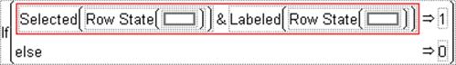
As Row State

Converts a numeric argument to a row state or set of row state conditions. Row states are stored internally in JMP as a 16-bit number, with each bit assigned to represent one of the possible row states as illustrated in Figure A.3. For example, the binary representation of 1327 is0000010100101111. As Row State(1327) would therefore set the row state as selected, excluded, hidden, labeled, with marker 2 and color 10.

Combine States

Generates a row state combination with two or more arguments. Use the insert button () on the Formula Editor keypad or type a comma to add arguments to the Combine States function. The currently selected expression becomes the first argument when you select Combine States.Replace each argument with an expression that evaluates to a row state. This formula:

Combine States(

Selected State(Modulo(Row(),2),

Labeled State(Modulo(Row()+1,2))

alternately labels or selects each row in the calculated row state column. The Selected State and Labeled State functions are defined later in this section. Use the insert () and delete ()buttons on the Formula Editor keypad to add more arguments or remove unwanted arguments.

If you include conflicting row states in a combination, the results are unpredictable.

Excluded State

Interprets a numeric argument as true or false. When an argument evaluates as true, the Excluded State function assigns the excluded condition as the value of the column for that row. For example, Excluded State(Modulo(Row(),2)) assigns the excluded row state as the value of the row state column for each odd numbered row.

Hidden State

Assigns the hidden row state condition when its argument is greater than zero. If the argument is zero, the value in the column for that row is not hidden.

Labeled State

Gives the labeled row state condition when its argument is greater than zero. If the argument is zero the row value in the column for that row is not labeled.

Color State

Returns the color from the JMP color map that corresponds to its integer argument. JMP colors are numbered 0 through 84. Zero maps to black.

Marker State

Returns markers from the JMP marker map that correspond to its integer argument. JMP markers are numbered 0 through 16. The formula Marker State(Row()) assigns all the row state markers in a repeating sequence determined by the current row number to the calculated row state column. A row state column can have multiple row states as a value.

Selected State

Gives the selected row state condition when its argument is greater than zero. If the argument is zero, the value in the column for that row is not selected.

Hue State

Returns the color from the JMP hue map that corresponds to its integer argument. JMP hues are numbered 0 through 11 but larger integers are treated as modulo 12. The Hue State function does not map to black, gray, or white. A hue of zero maps to red and hue of 11 maps to magenta. The formula on the left in Figure A.17 assigns row state colors in a chromatic spread based on the value of z. The Hue State function used with a row state data type column.

Shade State

Assigns five shade levels to a color or hue. A shade of –2 is darkest and shade of +2 is lightest. A shade of zero is a pure color. The formula on the right in Figure A.17 assigns shade values based on the value of z.

Figure A.17 Examples of Hue and Shade Functions

To assign all shades of all the colors in the colors palette, you need to use the Hue State and Shade State assignments together. The formula in Figure A.18 uses the Combine States function described at the beginning of this section. The first argument in the Combine States function is the Hue State formula shown previously, and the second argument is the Shade State formula. In addition, the Marker State function with an argument of 2 assigns the X marker to each row, and the Selected State function with an argument of 1 selects each row.

Figure A.18 Combine States Example For Using Both Hue State and Row State

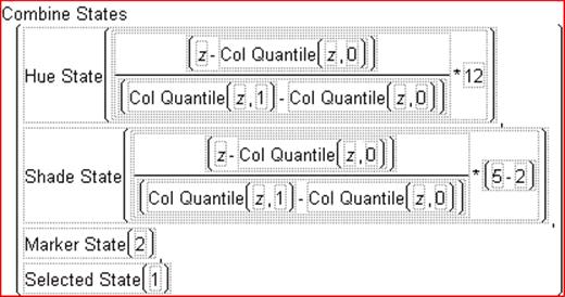
Excluded, Hidden, Labeled, and Selected

Accepts a row state expression argument (row state column or row state constant) that evaluates as either 1 or 0 (true or false). These characteristics are inactive by default. Often, the Row() function is the argument, which detects the active row state condition of each row. For example, inFigure A.19, the formula assigns 99 whenever a row is actively selected, and 0 otherwise. Note that this formula is used in a column that has a numeric data type.

Figure A.19 Example of a Formula Using the Selected Function

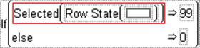
The example in Figure A.20 assigns row state conditions to a row state column. The formula for the row state column (in the column called x) checks to determine whether the active row state is either Hidden or Excluded, and if so, assigns the Labeled row state.

Figure A.20 Calculate Row State Information in a Row State Column

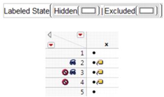
Color Of

Accepts any row state expression or column, or the Row State() function as its argument. Returns a number from the JMP color map that corresponds to the active color state, or zero if there is no assigned color.

Marker Of

Accepts any row state expression or column, or the Row State() function as its argument. Returns a number from the JMP marker map that corresponds to the active marker or zero if there is no assigned marker.

Assignment Functions

Assignment functions work in place. That is, the result returned by the operation (on the right of the operator) is stored in the argument on the left of the operator and replaces its current value.

Assignment statements are most often used in conjunction with other commands to build a JSL script. You can use the Formula Editor to create and execute a script in that column, but this is not recommended because of dependencies and ambiguities that can result. Most often, scripts are stored as .jsl files, and can be saved with a data table. See “Create and Save Scripts” in the “Enter and Edit Data” chapter. For details about syntax, see the Scripting Guide.

Note: The first argument of an assignment function must be capable of being assigned. This means you cannot have an assignment such as 3+=4, because 3 is a constant value that cannot be reassigned. You must first create a variable (a table variable or local variable) whose value is 3. (For details about table variables, see “Use Table Variables” in the “Enter and Edit Data” chapter. For details about local variables, see “Reference Columns and Table Variables” in the “Formula Editor” chapter). Then use that variable as the left-hand argument of the assignment function.

= (assign)

Puts the value of b into a. For example (a=b).

+= (add to)

Adds the value of b to a and puts the result back into a. For example, a+=b.

-= (subtract to)

Subtracts the value of b and puts the result back into a. For example, a–=b.

*= (multiply to)

Multiplies b with a and puts the result back into a. For example, a*=b.

/= (divide to)

Divides b into a and puts the result back into a. For example, a/=b.

++ (post increment)

Adds one (1) to a, in place, so that a++. For example, if the initial value of a is 4, the expression a++ changes a to 5.

-- (post decrement)

Subtracts one (1) from a, in place, so that a– – . For example, if the initial value of a is 4, the expression a– – changes a to 3.

Parametric Model Functions

This category is a short cut to create three parametric models that are linear functions of set of window-selected columns.

Linear Model, Interactions Model, Full Quadratic Model

Selecting each of these opens a column selection box that lets you select one or more columns to be included in the model. The function then creates and populates the chosen model.

Finance Functions

Lets you create formulas to calculate principal payments, interest rate, rate of return, and so on.

Double Declining Balance

Returns the depreciation of an asset for a specified period of time. The function uses the double-declining balance method or some other depreciation factor.

Future Value

Returns the future value of an investment that is based on periodic, constant payments and a constant interest rate.

Interest Payment

Returns the interest payment for a given period for an investment that is based on periodic, constant payments and a constant interest rate.

Interest Rate

Returns the interest rate per period of an annuity.

Internal Rate of Return

Returns the internal rate of return for a series of cash flows in the values argument.

Modified Internal Rate of Return

Returns the modified internal rate of return for a series of periodic cash flows. The cost of investment and the interest received on reinvested cash is included.

Net Present Value

Returns the net present value of an investment by using a discount rate and a series of future payments (negative values) and income (positive values).

Number of Periods

Returns the number of periods for an investment that is based on periodic, constant payments and a constant interest rate.

Payment

Returns the payment for a loan that is based on constant payments and a constant interest rate.

Present Value

Returns the present value of an investment.

Principal Payment

Returns the payment on the principal for a given period for an investment that is based on periodic, constant payments and a constant interest rate.

Straight Line Depreciation

Returns the straight-line depreciation of an asset for one period.

Sum Of Years Digits Depreciation

Returns the sum-of-years’ digits depreciation of an asset for a specified period.