Large Scale Machine Learning with Python (2016)
Chapter 9. Practical Machine Learning with Spark
In the previous chapter, we saw the main functionalities of data processing with Spark. In this chapter, we will focus on data science with Spark on a real data problem. During the chapter, you will learn the following topics:
· How to share variables across a cluster's nodes
· How to create DataFrames from structured (CSV) and semi-structured (JSON) files, save them on disk, and load them
· How to use SQL-like syntax to select, filter, join, group, and aggregate datasets, thus making the preprocessing extremely easy
· How to handle missing data in the dataset
· Which algorithms are available out of the box in Spark for feature engineering and how to use them in a real case scenario
· Which learners are available and how to measure their performance in a distributed environment
· How to run cross-validation for hyperparameter optimization in a cluster
Setting up the VM for this chapter
As machine learning needs a lot of computational power, in order to save some resources (especially memory) we will use the Spark environment not backed by YARN in this chapter. This mode of operation is named standalone and creates a Spark node without cluster functionalities; all the processing will be on the driver machine and won't be shared. Don't worry; the code that we will see in this chapter will work in a cluster environment as well.
In order to operate this way, perform the following steps:
1. Turn on the virtual machine using the vagrant up command.
2. Access the virtual machine when it's ready, with vagrant ssh.
3. Launch Spark standalone mode with the IPython Notebook from inside the virtual machine with ./start_jupyter.sh.
4. Open a browser pointing to http://localhost:8888.
To turn it off, use the Ctrl + C keys to exit the IPython Notebook and vagrant halt to turn off the virtual machine.
Note
Note that, even in this configuration, you can access the Spark UI (when at least an IPython Notebook is running) at the following URL:
http://localhost:4040
Sharing variables across cluster nodes
When we're working on a distributed environment, sometimes it is required to share information across nodes so that all the nodes can operate using consistent variables. Spark handles this case by providing two kinds of variables: read-only and write-only variables. By not ensuring that a shared variable is both readable and writable anymore, it also drops the consistency requirement, letting the hard work of managing this situation fall on the developer's shoulders. Usually, a solution is quickly reached as Spark is really flexible and adaptive.
Broadcast read-only variables
Broadcast variables are variables shared by the driver node, that is, the node running the IPython Notebook in our configuration, with all the nodes in the cluster. It's a read-only variable as the variable is broadcast by one node and never read back if another node changes it.
Let's now see how it works on a simple example: we want to one-hot encode a dataset containing just gender information as a string. Precisely, the dummy dataset contains just a feature that can be male M, female F, or unknown U (if the information is missing). Specifically, we want all the nodes to use a defined one-hot encoding, as listed in the following dictionary:
In:one_hot_encoding = {"M": (1, 0, 0),
"F": (0, 1, 0),
"U": (0, 0, 1)
}
Let's now try doing it step by step.
The easiest solution (it's not working though) is to parallelize the dummy dataset (or read it from the disk) and then use the map method on the RDD with a lambda function to map a gender to its encoded tuple:
In:(sc.parallelize(["M", "F", "U", "F", "M", "U"])
.map(lambda x: one_hot_encoding[x])
.collect())
Out:
[(1, 0, 0), (0, 1, 0), (0, 0, 1), (0, 1, 0), (1, 0, 0), (0, 0, 1)]
This solution works locally, but it won't operate on a real distributed environment as all the nodes don't have the one_hot_encoding variable available in their workspace. A quick workaround is to include the Python dictionary in the mapped function (that's distributed) as we manage to do here:
In:
def map_ohe(x):
ohe = {"M": (1, 0, 0),
"F": (0, 1, 0),
"U": (0, 0, 1)
}
return ohe[x]
sc.parallelize(["M", "F", "U", "F", "M", "U"]).map(map_ohe).collect()
Out:
[(1, 0, 0), (0, 1, 0), (0, 0, 1), (0, 1, 0), (1, 0, 0), (0, 0, 1)] here are you I love you hello hi is that email with all leave formal minutes very worrying A hey
Such a solution works both locally and on the server, but it's not very nice: we mixed data and process, making the mapping function not reusable. It would be better if the mapping function refers to a broadcasted variable so that it can be used with whatsoever mapping we need to one-hot encode the dataset.
For this, we first broadcast the Python dictionary (calling the broadcast method provided by the Spark context, sc) inside the mapped function; using its .value property, we can now have access to it. After doing this, we have a generic map function that can work on any one-hot map dictionary:
In:bcast_map = sc.broadcast(one_hot_encoding)
def bcast_map_ohe(x, shared_ohe):
return shared_ohe[x]
(sc.parallelize(["M", "F", "U", "F", "M", "U"])
.map(lambda x: bcast_map_ohe(x, bcast_map.value))
.collect())
Out:
[(1, 0, 0), (0, 1, 0), (0, 0, 1), (0, 1, 0), (1, 0, 0), (0, 0, 1)]
Think about the broadcasted variable as a file written in HDFS. Then, when a generic node wants to access it, it just needs the HDFS path (which is passed as an argument of the map method) and you're sure that all of them will read the same thing, using the same path. Of course, Spark doesn't use HDFS, but an in-memory variation of it.
Note
Broadcasted variables are saved in-memory in all the nodes composing a cluster; therefore, they never share a large amount of data that can fill them and make the following processing impossible.
To remove a broadcasted variable, use the unpersist method on the broadcasted variable. This operation will free up the memory of that variable on all the nodes:
In:bcast_map.unpersist()
Accumulators write-only variables
The other variables that can be shared in a Spark cluster are accumulators. Accumulators are write-only variables that can be added together and are used typically to implement sums or counters. Just the driver node, the one that is running the IPython Notebook, can read its value; all the other nodes can't.
Let's see how it works using an example: we want to process a text file and understand how many lines are empty while processing it. Of course, we can do this by scanning the dataset twice (using two Spark jobs): the first one counting the empty lines, and the second time doing the real processing, but this solution is not very effective.
In the first, ineffective solution—extracting the number of empty lines using two standalone Spark jobs—we can read the text file, filter the empty lines, and count them, as shown here:
In:print "The number of empty lines is:"
(sc.textFile('file:///home/vagrant/datasets/hadoop_git_readme.txt')
.filter(lambda line: len(line) == 0)
.count())
Out:The number of empty lines is:
6
The second solution is instead more effective (and more complex). We instantiate an accumulator variable (with the initial value of 0) and we add 1 for each empty line that we find while processing each line of the input file (with a map). At the same time, we can do some processing on each line; in the following piece of code, for example, we simply return 1 for each line, counting all the lines in the file in this way.
At the end of the processing, we will have two pieces of information: the first is the number of lines, from the result of the count() action on the transformed RDD, and the second is the number of empty lines contained in the value property of the accumulator. Remember, both of these are available after having scanned the dataset once:
In:accum = sc.accumulator(0)
def split_line(line):
if len(line) == 0:
accum.add(1)
return 1
tot_lines = (
sc.textFile('file:///home/vagrant/datasets/hadoop_git_readme.txt')
.map(split_line)
.count())
empty_lines = accum.value
print "In the file there are %d lines" % tot_lines
print "And %d lines are empty" % empty_lines
Out:In the file there are 31 lines And 6 lines are empty
Natively, Spark supports accumulators of numeric types, and the default operation is a sum. With a bit more coding, we can turn it into something more complex.
Broadcast and accumulators together – an example
Although broadcast and accumulators are simple and very limited variables (one is read-only, the other one is write-only), they can be actively used to create very complex operations. For example, let's try to apply different machine learning algorithms on the Iris dataset in a distributed environment. We will build a Spark job in the following way:
1. The dataset is read and broadcasted to all the nodes (as it's small enough to fit in-memory).
2. Each node will use a different classifier on the dataset and return the classifier name and its accuracy score on the full dataset. Note that, to keep things easy in this simple example, we won't do any preprocessing, train/test splitting, or hyperparameter optimization.
3. If the classifiers raise any exception, the string representation of the error along with the classifier name should be stored in an accumulator.
4. The final output should contain a list of the classifiers that performed the classification task without errors and their accuracy score.
As the first step, we load the Iris dataset and broadcast it to all the nodes in the cluster:
In:from sklearn.datasets import load_iris
bcast_dataset = sc.broadcast(load_iris())
Now, let's create a custom accumulator. It will contain a list of tuples to store the classifier name and the exception it experienced as a string. The custom accumulator is derived by the AccumulatorParam class and should contain at least two methods: zero (which is called when it's initialized) and addInPlace (which is called when the add method is called on the accumulator).
The easiest way to do this is shown in the following code, followed by its initialization as an empty list. Mind that the additive operation is a bit tricky: we need to combine two elements, a tuple, and a list, but we don't know which element is the list and which is the tuple; therefore, we first ensure that both elements are lists and then we can proceed to concatenate them in an easy way (with the + operator):
In:from pyspark import AccumulatorParam
class ErrorAccumulator(AccumulatorParam):
def zero(self, initialList):
return initialList
def addInPlace(self, v1, v2):
if not isinstance(v1, list):
v1 = [v1]
if not isinstance(v2, list):
v2 = [v2]
return v1 + v2
errAccum = sc.accumulator([], ErrorAccumulator())
Now, let's define the mapping function: each node should train, test, and evaluate a classifier on the broadcasted Iris dataset. As an argument, the function will receive the classifier object and should return a tuple containing the classifier name and its accuracy score contained in a list.
If any exception is raised by doing so, the classifier name and exception as a string are added to the accumulator, and it's returned as an empty list:
In:
def apply_classifier(clf, dataset):
clf_name = clf.__class__.__name__
X = dataset.value.data
y = dataset.value.target
try:
from sklearn.metrics import accuracy_score
clf.fit(X, y)
y_pred = clf.predict(X)
acc = accuracy_score(y, y_pred)
return [(clf_name, acc)]
except Exception as e:
errAccum.add((clf_name, str(e)))
return []
Finally, we have arrived at the core of the job. We're now instantiating a few objects from Scikit-learn (some of them are not classifiers, in order to test the accumulator). We will transform them into an RDD and apply the map function that we created in the previous cell. As the returned value is a list, we can use flatMap to collect just the outputs of the mappers that didn't get caught in any exception:
In:from sklearn.linear_model import SGDClassifier
from sklearn.dummy import DummyClassifier
from sklearn.decomposition import PCA
from sklearn.manifold import MDS
classifiers = [DummyClassifier('most_frequent'),
SGDClassifier(),
PCA(),
MDS()]
(sc.parallelize(classifiers)
.flatMap(lambda x: apply_classifier(x, bcast_dataset))
.collect())
Out:[('DummyClassifier', 0.33333333333333331),
('SGDClassifier', 0.66666666666666663)]
As expected, only the real classifiers are contained in the output. Let's now see which classifiers generated an error. Unsurprisingly, here we spot the two missing ones from the preceding output:
In:print "The errors are:"
errAccum.value
Out:The errors are:
[('PCA', "'PCA' object has no attribute 'predict'"),
('MDS', "Proximity must be 'precomputed' or 'euclidean'. Got euclidean instead")]
As a final step, let's clean up the broadcasted dataset:
In:bcast_dataset.unpersist()
Remember that in this example, we've used a small dataset that could be broadcasted. In real-world big data problems, you'll need to load the dataset from HDFS, broadcasting the HDFS path.
Data preprocessing in Spark
So far, we've seen how to load text data from the local filesystem and HDFS. Text files can contain either unstructured data (like a text document) or structured data (like a CSV file). As for semi-structured data, just like files containing JSON objects, Spark has special routines able to transform a file into a DataFrame, similar to the DataFrame in R and Python pandas. DataFrames are very similar to RDBMS tables, where a schema is set.
JSON files and Spark DataFrames
In order to import JSON-compliant files, we should first create a SQL context, creating a SQLContext object from the local Spark Context:
In:from pyspark.sql import SQLContext
sqlContext = SQLContext(sc)
Now, let's see the content of a small JSON file (it's provided in the Vagrant virtual machine). It's a JSON representation of a table with six rows and three columns, where some attributes are missing (such as the gender attribute for the user with user_id=0):
In:!cat /home/vagrant/datasets/users.json
Out:{"user_id":0, "balance": 10.0}
{"user_id":1, "gender":"M", "balance": 1.0}
{"user_id":2, "gender":"F", "balance": -0.5}
{"user_id":3, "gender":"F", "balance": 0.0}
{"user_id":4, "balance": 5.0}
{"user_id":5, "gender":"M", "balance": 3.0}
Using the read.json method provided by sqlContext, we already have the table well formatted and with all the right column names in a variable. The output variable is typed as Spark DataFrame. To show the variable in a nice, formatted table, use its show method:
In:
df = sqlContext.read \
.json("file:///home/vagrant/datasets/users.json")
df.show()
Out:
+-------+------+-------+
|balance|gender|user_id|
+-------+------+-------+
| 10.0| null| 0|
| 1.0| M| 1|
| -0.5| F| 2|
| 0.0| F| 3|
| 5.0| null| 4|
| 3.0| M| 5|
+-------+------+-------+
Additionally, we can investigate the schema of the DataFrame using the printSchema method. We realize that, while reading the JSON file, each column type has been inferred by the data (in the example, the user_id column contains long integers, the gender column is composed by strings, and the balance is a double floating point):
In:df.printSchema()
Out:root
|-- balance: double (nullable = true)
|-- gender: string (nullable = true)
|-- user_id: long (nullable = true)
Exactly like a table in an RDBMS, we can slide and dice the data in the DataFrame, making selections of columns and filtering the data by attributes. In this example, we want to print the balance, gender, and user_id of the users whose gender is not missing and have a balance strictly greater than zero. For this, we can use the filter and select methods:
In:(df.filter(df['gender'] != 'null')
.filter(df['balance'] > 0)
.select(['balance', 'gender', 'user_id'])
.show())
Out:
+-------+------+-------+
|balance|gender|user_id|
+-------+------+-------+
| 1.0| M| 1|
| 3.0| M| 5|
+-------+------+-------+
We can also rewrite each piece of the preceding job in a SQL-like language. In fact, filter and select methods can accept SQL-formatted strings:
In:(df.filter('gender is not null')
.filter('balance > 0').select("*").show())
Out:
+-------+------+-------+
|balance|gender|user_id|
+-------+------+-------+
| 1.0| M| 1|
| 3.0| M| 5|
+-------+------+-------+
We can also use just one call to the filter method:
In:df.filter('gender is not null and balance > 0').show()
Out:
+-------+------+-------+
|balance|gender|user_id|
+-------+------+-------+
| 1.0| M| 1|
| 3.0| M| 5|
+-------+------+-------+
Dealing with missing data
A common problem of data preprocessing is to handle missing data. Spark DataFrames, similar to pandas DataFrames, offer a wide range of operations that you can do on them. For example, the easiest option to have a dataset composed by complete rows only is to discard rows containing missing information. For this, in a Spark DataFrame, we first have to access the na attribute of the DataFrame and then call the drop method. The resulting table will contain only the complete rows:
In:df.na.drop().show()
Out:
+-------+------+-------+
|balance|gender|user_id|
+-------+------+-------+
| 1.0| M| 1|
| -0.5| F| 2|
| 0.0| F| 3|
| 3.0| M| 5|
+-------+------+-------+
If such an operation is removing too many rows, we can always decide what columns should be accounted for the removal of the row (as the augmented subset of the drop method):
In:df.na.drop(subset=["gender"]).show()
Out:
+-------+------+-------+
|balance|gender|user_id|
+-------+------+-------+
| 1.0| M| 1|
| -0.5| F| 2|
| 0.0| F| 3|
| 3.0| M| 5|
+-------+------+-------+
Also, if you want to set default values for each column instead of removing the line data, you can use the fill method, passing a dictionary composed by the column name (as the dictionary key) and the default value to substitute missing data in that column (as the value of the key in the dictionary).
As an example, if you want to ensure that the variable balance, where missing, is set to 0, and the variable gender, where missing, is set to U, you can simply do the following:
In:df.na.fill({'gender': "U", 'balance': 0.0}).show()
Out:
+-------+------+-------+
|balance|gender|user_id|
+-------+------+-------+
| 10.0| U| 0|
| 1.0| M| 1|
| -0.5| F| 2|
| 0.0| F| 3|
| 5.0| U| 4|
| 3.0| M| 5|
+-------+------+-------+
Grouping and creating tables in-memory
To have a function applied on a group of rows (exactly as in the case of SQL GROUP BY), you can use two similar methods. In the following example, we want to compute the average balance per gender:
In:(df.na.fill({'gender': "U", 'balance': 0.0})
.groupBy("gender").avg('balance').show())
Out:
+------+------------+
|gender|avg(balance)|
+------+------------+
| F| -0.25|
| M| 2.0|
| U| 7.5|
+------+------------+
So far, we've worked with DataFrames but, as you've seen, the distance between DataFrame methods and SQL commands is minimal. Actually, using Spark, it is possible to register the DataFrame as a SQL table to fully enjoy the power of SQL. The table is saved in-memory and distributed in a way similar to an RDD.
To register the table, we need to provide a name, which will be used in future SQL commands. In this case, we decide to name it users:
In:df.registerTempTable("users")
By calling the sql method provided by the Spark sql context, we can run any SQL-compliant table:
In:sqlContext.sql("""
SELECT gender, AVG(balance)
FROM users
WHERE gender IS NOT NULL
GROUP BY gender""").show()
Out:
+------+-----+
|gender| _c1|
+------+-----+
| F|-0.25|
| M| 2.0|
+------+-----+
Not surprisingly, the table outputted by the command (as well as the users table itself) is of the Spark DataFrame type:
In:type(sqlContext.table("users"))
Out:pyspark.sql.dataframe.DataFrame
DataFrames, tables, and RDDs are intimately connected, and RDD methods can be used on a DataFrame. Remember that each row of the DataFrame is an element of the RDD. Let's see this in detail and first collect the whole table:
In:sqlContext.table("users").collect()
Out:[Row(balance=10.0, gender=None, user_id=0),
Row(balance=1.0, gender=u'M', user_id=1),
Row(balance=-0.5, gender=u'F', user_id=2),
Row(balance=0.0, gender=u'F', user_id=3),
Row(balance=5.0, gender=None, user_id=4),
Row(balance=3.0, gender=u'M', user_id=5)]
In:
a_row = sqlContext.sql("SELECT * FROM users").first()
a_row
Out:Row(balance=10.0, gender=None, user_id=0)
The output is a list of Row objects (they look like Python's namedtuple). Let's dig deeper into it: Row contains multiple attributes, and it's possible to access them as a property or dictionary key; that is, to have the balance out from the first row, we can choose between the two following ways:
In:print a_row['balance']
print a_row.balance
Out:10.0
10.0
Also, Row can be collected as a Python dictionary using the asDict method of Row. The result contains the property names as a key and property values as dictionary values:
In:a_row.asDict()
Out:{'balance': 10.0, 'gender': None, 'user_id': 0}
Writing the preprocessed DataFrame or RDD to disk
To write a DataFrame or RDD to disk, we can use the write method. We have a selection of formats; in this case, we will save it as a JSON file on the local machine:
In:(df.na.drop().write
.save("file:///tmp/complete_users.json", format='json'))
Checking the output on the local filesystem, we immediately see that something is different from what we expected: this operation creates multiple files (part-r-…).
Each of them contains some rows serialized as JSON objects, and merging them together will create the comprehensive output. As Spark is made to process large and distributed files, the write operation is tuned for that and each node writes part of the full RDD:
In:!ls -als /tmp/complete_users.json
Out:total 28
4 drwxrwxr-x 2 vagrant vagrant 4096 Feb 25 22:54 .
4 drwxrwxrwt 9 root root 4096 Feb 25 22:54 ..
4 -rw-r--r-- 1 vagrant vagrant 83 Feb 25 22:54 part-r-00000-...
4 -rw-rw-r-- 1 vagrant vagrant 12 Feb 25 22:54 .part-r-00000-...
4 -rw-r--r-- 1 vagrant vagrant 82 Feb 25 22:54 part-r-00001-...
4 -rw-rw-r-- 1 vagrant vagrant 12 Feb 25 22:54 .part-r-00001-...
0 -rw-r--r-- 1 vagrant vagrant 0 Feb 25 22:54 _SUCCESS
4 -rw-rw-r-- 1 vagrant vagrant 8 Feb 25 22:54 ._SUCCESS.crc
In order to read it back, we don't have to create a standalone file—even multiple pieces are fine in the read operation. A JSON file can also be read in the FROM clause of a SQL query. Let's now try to print the JSON that we've just written on disk without creating an intermediate DataFrame:
In:sqlContext.sql(
"SELECT * FROM json.`file:///tmp/complete_users.json`").show()
Out:
+-------+------+-------+
|balance|gender|user_id|
+-------+------+-------+
| 1.0| M| 1|
| -0.5| F| 2|
| 0.0| F| 3|
| 3.0| M| 5|
+-------+------+-------+
Beyond JSON, there is another format that's very popular when dealing with structured big datasets: Parquet format. Parquet is a columnar storage format that's available in the Hadoop ecosystem; it compresses and encodes the data and can work with nested structures: all such qualities make it very efficient.
Saving and loading is very similar to JSON and, even in this case, this operation produces multiple files written to disk:
In:df.na.drop().write.save(
"file:///tmp/complete_users.parquet", format='parquet')
In:!ls -als /tmp/complete_users.parquet/
Out:total 44
4 drwxrwxr-x 2 vagrant vagrant 4096 Feb 25 22:54 .
4 drwxrwxrwt 10 root root 4096 Feb 25 22:54 ..
4 -rw-r--r-- 1 vagrant vagrant 376 Feb 25 22:54 _common_metadata
4 -rw-rw-r-- 1 vagrant vagrant 12 Feb 25 22:54 ._common_metadata..
4 -rw-r--r-- 1 vagrant vagrant 1082 Feb 25 22:54 _metadata
4 -rw-rw-r-- 1 vagrant vagrant 20 Feb 25 22:54 ._metadata.crc
4 -rw-r--r-- 1 vagrant vagrant 750 Feb 25 22:54 part-r-00000-...
4 -rw-rw-r-- 1 vagrant vagrant 16 Feb 25 22:54 .part-r-00000-...
4 -rw-r--r-- 1 vagrant vagrant 746 Feb 25 22:54 part-r-00001-...
4 -rw-rw-r-- 1 vagrant vagrant 16 Feb 25 22:54 .part-r-00001-...
0 -rw-r--r-- 1 vagrant vagrant 0 Feb 25 22:54 _SUCCESS
4 -rw-rw-r-- 1 vagrant vagrant 8 Feb 25 22:54 ._SUCCESS.crc
Working with Spark DataFrames
So far, we've described how to load DataFrames from JSON and Parquet files, but not how to create them from an existing RDD. In order to do so, you just need to create one Row object for each record in the RDD and call the createDataFrame method of the SQL context. Finally, you can register it as a temp table to use the power of the SQL syntax fully:
In:from pyspark.sql import Row
rdd_gender = \
sc.parallelize([Row(short_gender="M", long_gender="Male"),
Row(short_gender="F", long_gender="Female")])
(sqlContext.createDataFrame(rdd_gender)
.registerTempTable("gender_maps"))
In:sqlContext.table("gender_maps").show()
Out:
+-----------+------------+
|long_gender|short_gender|
+-----------+------------+
| Male| M|
| Female| F|
+-----------+------------+
Note
This is also the preferred way to operate with CSV files. First, the file is read with sc.textFile; then with the split method, the Row constructor, and the createDataFrame method, the final DataFrame is created.
When you have multiple DataFrames in-memory, or that can be loaded from disk, you can join and use all the operations available in a classic RDBMS. In this example, we can join the DataFrame we've created from the RDD with the users dataset contained in the Parquet file that we've stored. The result is astonishing:
In:sqlContext.sql("""
SELECT balance, long_gender, user_id
FROM parquet.`file:///tmp/complete_users.parquet`
JOIN gender_maps ON gender=short_gender""").show()
Out:
+-------+-----------+-------+
|balance|long_gender|user_id|
+-------+-----------+-------+
| 3.0| Male| 5|
| 1.0| Male| 1|
| 0.0| Female| 3|
| -0.5| Female| 2|
+-------+-----------+-------+
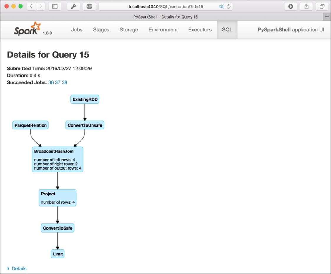
In the web UI, each SQL query is mapped as a virtual directed acyclic graph (DAG) under the SQL tab. This is very nice to keep track of the progress of your job and understand the complexity of the query. While doing the preceding JOIN query, you can clearly see that two branches are entering the same BroadcastHashJoin block: the first one is from an RDD and the second one is from a Parquet file. Then, the following block is simply a projetion on the selected columns:
As the tables are in-memory, the last thing to do is to clean up releasing the memory used to keep them. By calling the tableNames method, provided by the sqlContext, we have the list of all the tables that we currently have in-memory. Then, to free them up, we can use dropTempTable with the name of the table as argument. Beyond this point, any further reference to these tables will return an error:
In:sqlContext.tableNames()
Out:[u'gender_maps', u'users']
In:
for table in sqlContext.tableNames():
sqlContext.dropTempTable(table)
Since Spark 1.3, DataFrame is the preferred way to operate on a dataset when doing data science operations.
Machine learning with Spark
Here, we arrive at the main task of your job: creating a model to predict one or multiple attributes missing in the dataset. For this, we use some machine learning modeling, and Spark can provide us with a big hand in this context.
MLlib is the Spark machine learning library; although it is built in Scala and Java, its functions are also available in Python. It contains classification, regression, and recommendation learners, some routines for dimensionality reduction and feature selection, and has lots of functionalities for text processing. All of them are able to cope with huge datasets and use the power of all the nodes in the cluster to achieve the goal.
As of now (2016), it's composed of two main packages: mllib, which operates on RDDs, and ml, which operates on DataFrames. As the latter performs well and the most popular way to represent data in data science, developers have chosen to contribute and improve the ml branch, letting the former remain, but without further developments. MLlib seems a complete library at first sight but, after having started using Spark, you will notice that there's neither a statistic nor numerical library in the default package. Here, SciPy and NumPy come to your help, and once again, they're essential for data science!
In this section, we will try to explore the functionalities of the new pyspark.ml package; as of now, it's still in the early stages compared to the state-of-the-art Scikit-learn library, but it definitely has a lot of potential for the future.
Note
Spark is a high-level, distributed, and complex software that should be used just on big data and with a cluster of multiple nodes; in fact, if the dataset can fit in-memory, it's more convenient to use other libraries such as Scikit-learn or similar, which focus just on the data science side of the problem. Running Spark on a single node on a small dataset can be five times slower than the Scikit-learn-equivalent algorithm.
Spark on the KDD99 dataset
Let's conduct this exploration using a real-world dataset: the KDD99 dataset. The goal of the competition was to create a network intrusion detection system able to recognize which network flow is malicious and which is not. Moreover, many different attacks are in the dataset; the goal is to accurately predict them using the features of the flow of packets contained in the dataset.
As a side node on the dataset, it has been extremely useful to develop great solutions for intrusion detection systems in the first few years after its release. Nowadays, as an outcome of this, all the attacks included in the dataset are very easy to detect and so it's not used in IDS development anymore.
The features are, for example, the protocol (tcp, icmp, and udp), service (http, smtp, and so on), size of the packets, flags active in the protocol, number of attempts to become root, and so on.
Note
More information about the KDD99 challenge and datasets is available at http://kdd.ics.uci.edu/databases/kddcup99/kddcup99.html.
Although this is a classic multiclass classification problem, we will dig into it to show you how to perform this task in Spark. To keep things clean, we will use a new IPython Notebook.
Reading the dataset
First at all, let's download and decompress the dataset. We will be very conservative and use just 10% of the original training dataset (75MB, uncompressed) as all our analysis is run on a small virtual machine. If you want to give it a try, you can uncomment the lines in the following snippet of code and download the full training dataset (750MB uncompressed). We download the training dataset, testing (47MB), and feature names, using bash commands:
In:!rm -rf ../datasets/kdd*
# !wget -q -O ../datasets/kddtrain.gz \
# http://kdd.ics.uci.edu/databases/kddcup99/kddcup.data.gz
!wget -q -O ../datasets/kddtrain.gz \
http://kdd.ics.uci.edu/databases/kddcup99/kddcup.data_10_percent.gz
!wget -q -O ../datasets/kddtest.gz \
http://kdd.ics.uci.edu/databases/kddcup99/corrected.gz
!wget -q -O ../datasets/kddnames \
http://kdd.ics.uci.edu/databases/kddcup99/kddcup.names
!gunzip ../datasets/kdd*gz
Now, print the first few lines to have an understanding of the format. It is clear that it's a classic CSV without a header, containing a dot at the end of each line. Also, we can see that some fields are numeric but a few of them are textual, and the target variable is contained in the last field:
In:!head -3 ../datasets/kddtrain
Out:
0,tcp,http,SF,181,5450,0,0,0,0,0,1,0,0,0,0,0,0,0,0,0,0,8,8,0.00,0.00,0.00,0.00,1.00,0.00,0.00,9,9,1.00,0.00,0.11,0.00,0.00,0.00,0.00,0.00,normal.
0,tcp,http,SF,239,486,0,0,0,0,0,1,0,0,0,0,0,0,0,0,0,0,8,8,0.00,0.00,0.00,0.00,1.00,0.00,0.00,19,19,1.00,0.00,0.05,0.00,0.00,0.00,0.00,0.00,normal.
0,tcp,http,SF,235,1337,0,0,0,0,0,1,0,0,0,0,0,0,0,0,0,0,8,8,0.00,0.00,0.00,0.00,1.00,0.00,0.00,29,29,1.00,0.00,0.03,0.00,0.00,0.00,0.00,0.00,normal.
To create a DataFrame with named fields, we should first read the header included in the kddnames file. The target field will be named simply target.
After having read and parsed the file, we print the number of features of our problem (remember that the target variable is not a feature) and their first 10 names:
In:
with open('../datasets/kddnames', 'r') as fh:
header = [line.split(':')[0]
for line in fh.read().splitlines()][1:]
header.append('target')
print "Num features:", len(header)-1
print "First 10:", header[:10]
Out:Num features: 41
First 10: ['duration', 'protocol_type', 'service', 'flag', 'src_bytes', 'dst_bytes', 'land', 'wrong_fragment', 'urgent', 'hot']
Let's now create two separate RDDs—one for the training data and the other for the testing data:
In:
train_rdd = sc.textFile('file:///home/vagrant/datasets/kddtrain')
test_rdd = sc.textFile('file:///home/vagrant/datasets/kddtest')
Now, we need to parse each line of each file to create a DataFrame. First, we split each line of the CSV file into separate fields, and then we cast each numerical value to a floating point and each text value to a string. Finally, we remove the dot at the end of each line.
As the last step, using the createDataFrame method provided by sqlContext, we can create two Spark DataFrames with named columns for both training and testing datasets:
In:
def line_parser(line):
def piece_parser(piece):
if "." in piece or piece.isdigit():
return float(piece)
else:
return piece
return [piece_parser(piece) for piece in line[:-1].split(',')]
train_df = sqlContext.createDataFrame(
train_rdd.map(line_parser), header)
test_df = sqlContext.createDataFrame(
test_rdd.map(line_parser), header)
So far we've written just RDD transformers; let's introduce an action to see how many observations we have in the datasets and, at the same time, check the correctness of the previous code.
In:print "Train observations:", train_df.count()
print "Test observations:", test_df.count()
Out:Train observations: 494021
Test observations: 311029
Although we're using a tenth of the full KDD99 dataset, we still work on half a million observations. Multiplied by the number of features, 41, we clearly see that we'll be training our classifier on an observation matrix containing more than 20 million values. This is not such a big dataset for Spark (and neither is the full KDD99); developers around the world are already using it on petabytes and billion records. Don't be scared if the numbers seem big: Spark is designed to cope with them!
Now, let's see how it looks on the schema of the DataFrame. Specifically, we want to identify which fields are numeric and which contain strings (note that the result has been truncated for brevity):
In:train_df.printSchema()
Out:root
|-- duration: double (nullable = true)
|-- protocol_type: string (nullable = true)
|-- service: string (nullable = true)
|-- flag: string (nullable = true)
|-- src_bytes: double (nullable = true)
|-- dst_bytes: double (nullable = true)
|-- land: double (nullable = true)
|-- wrong_fragment: double (nullable = true)
|-- urgent: double (nullable = true)
|-- hot: double (nullable = true)
...
...
...
|-- target: string (nullable = true)
Feature engineering
From a visual analysis, only four fields are strings: protocol_type, service, flag, and target (which is the multiclass target label, as expected).
As we will use a tree-based classifier, we want to encode the text of each level to a number for each variable. With Scikit-learn, this operation can be done with a sklearn.preprocessing.LabelEncoder object. It's equivalent in Spark is StringIndexer of thepyspark.ml.feature package.
We need to encode four variables with Spark; then we have to chain four StringIndexer objects together in a cascade: each of them will operate on a specific column of the DataFrame, outputting a DataFrame with an additional column (similar to a map operation). The mapping is automatic, ordered by frequency: Spark ranks the count of each level in the selected column, mapping the most popular level to 0, the next to 1, and so on. Note that, with this operation, you will traverse the dataset once to count the occurrences of each level; if you already know the mapping, it would be more effective to broadcast it and use a map operation, as shown at the beginning of this chapter.
Similarly, we could have used a one-hot encoder to generate a numerical observation matrix. In case of a one-hot encoder, we would have had multiple output columns in the DataFrame, one for each level of each categorical feature. For this, Spark offers thepyspark.ml.feature.OneHotEncoder class.
Note
More generically, all the classes contained in the pyspark.ml.feature package are used to extract, transform, and select features from a DataFrame. All of them read some columns and create some other columns in the DataFrame.
As of Spark 1.6, the feature operations available in Python are contained in the following exhaustive list (all of them can be found in the pyspark.ml.feature package). Names should be intuitive, except for a couple of them that will be explained inline or later in the text:
· For text inputs (ideally):
· HashingTF and IDF
· Tokenizer and its regex-based implementation, RegexTokenizer
· Word2vec
· StopWordsRemover
· Ngram
· For categorical features:
· StringIndexer and it's inverse encoder, IndexToString
· OneHotEncoder
· VectorIndexer (out-of-the-box categorical to numerical indexer)
· For other inputs:
· Binarizer
· PCA
· PolynomialExpansion
· Normalizer, StandardScaler, and MinMaxScaler
· Bucketizer (buckets the values of a feature)
· ElementwiseProduct (multiplies columns together)
· Generic:
· SQLTransformer (implements transformations defined by a SQL statement, referring to DataFrame as a table named __THIS__)
· RFormula (selects columns using an R-style syntax)
· VectorAssembler (creates a feature vector from multiple columns)
Going back to the example, we now want to encode the levels in each categorical variable as discrete numbers. As we've explained, for this, we will use a StringIndexer object for each variable. Moreover, we can use an ML Pipeline and set them as stages of it.
Then, to fit all the indexers, you just need to call the fit method of the pipeline. Internally, it will fit all the staged objects sequentially. When it's completed the fit operation, a new object is created and we can refer to it as the fitted pipeline. Calling the transformmethod of this new object will sequentially call all the staged elements (which are already fitted), each after the previous one is completed. In this snippet of code, you'll see the pipeline in action. Note that transformers compose the pipeline. Therefore, as no actions are present, nothing is actually executed. In the output DataFrame, you'll note four additional columns named the same as the original categorical ones, but with the _cat suffix:
In:from pyspark.ml import Pipeline
from pyspark.ml.feature import StringIndexer
cols_categorical = ["protocol_type", "service", "flag","target"]
preproc_stages = []
for col in cols_categorical:
out_col = col + "_cat"
preproc_stages.append(
StringIndexer(
inputCol=col, outputCol=out_col, handleInvalid="skip"))
pipeline = Pipeline(stages=preproc_stages)
indexer = pipeline.fit(train_df)
train_num_df = indexer.transform(train_df)
test_num_df = indexer.transform(test_df)
Let's investigate the pipeline a bit more. Here, we will see the stages in the pipeline: unfit pipeline and fitted pipeline. Note that there's a big difference between Spark and Scikit-learn: in Scikit-learn, fit and transform are called on the same object, and in Spark, thefit method produces a new object (typically, its name is added with a Model suffix, just as for Pipeline and PipelineModel), where you'll be able to call the transform method. This difference is derived from closures—a fitted object is easy to distribute across processes and the cluster:
In:print pipeline.getStages()
print pipeline
print indexer
Out:
[StringIndexer_432c8aca691aaee949b8, StringIndexer_4f10bbcde2452dd1b771, StringIndexer_4aad99dc0a3ff831bea6, StringIndexer_4b369fea07873fc9c2a3]
Pipeline_48df9eed31c543ba5eba
PipelineModel_46b09251d9e4b117dc8d
Let's see how the first observation, that is, the first line in the CSV file, changes after passing through the pipeline. Note that we use an action here, therefore all the stages in the pipeline and in the pipeline model are executed:
In:print "First observation, after the 4 StringIndexers:\n"
print train_num_df.first()
Out:First observation, after the 4 StringIndexers:
Row(duration=0.0, protocol_type=u'tcp', service=u'http', flag=u'SF', src_bytes=181.0, dst_bytes=5450.0, land=0.0, wrong_fragment=0.0, urgent=0.0, hot=0.0, num_failed_logins=0.0, logged_in=1.0, num_compromised=0.0, root_shell=0.0, su_attempted=0.0, num_root=0.0, num_file_creations=0.0, num_shells=0.0, num_access_files=0.0, num_outbound_cmds=0.0, is_host_login=0.0, is_guest_login=0.0, count=8.0, srv_count=8.0, serror_rate=0.0, srv_serror_rate=0.0, rerror_rate=0.0, srv_rerror_rate=0.0, same_srv_rate=1.0, diff_srv_rate=0.0, srv_diff_host_rate=0.0, dst_host_count=9.0, dst_host_srv_count=9.0, dst_host_same_srv_rate=1.0, dst_host_diff_srv_rate=0.0, dst_host_same_src_port_rate=0.11, dst_host_srv_diff_host_rate=0.0, dst_host_serror_rate=0.0, dst_host_srv_serror_rate=0.0, dst_host_rerror_rate=0.0, dst_host_srv_rerror_rate=0.0, target=u'normal', protocol_type_cat=1.0, service_cat=2.0, flag_cat=0.0, target_cat=2.0)
The resulting DataFrame looks very complete and easy to understand: all the variables have names and values. We immediately note that the categorical features are still there, for instance, we have both protocol_type (categorical) and protocol_type_cat (the numerical version of the variable mapped from categorical).
Extracting some columns from the DataFrame is as easy as using SELECT in a SQL query. Let's now build a list of names for all the numerical features: starting from the names found in the header, we remove the categorical ones and replace them with the numerically-derived. Finally, as we want just the features, we remove the target variable and its numerical-derived equivalent:
In:features_header = set(header) \
- set(cols_categorical) \
| set([c + "_cat" for c in cols_categorical]) \
- set(["target", "target_cat"])
features_header = list(features_header)
print features_header
print "Total numerical features:", len(features_header)
Out:['num_access_files', 'src_bytes', 'srv_count', 'num_outbound_cmds', 'rerror_rate', 'urgent', 'protocol_type_cat', 'dst_host_same_srv_rate', 'duration', 'dst_host_diff_srv_rate', 'srv_serror_rate', 'is_host_login', 'wrong_fragment', 'serror_rate', 'num_compromised', 'is_guest_login', 'dst_host_rerror_rate', 'dst_host_srv_serror_rate', 'hot', 'dst_host_srv_count', 'logged_in', 'srv_rerror_rate', 'dst_host_srv_diff_host_rate', 'srv_diff_host_rate', 'dst_host_same_src_port_rate', 'root_shell', 'service_cat', 'su_attempted', 'dst_host_count', 'num_file_creations', 'flag_cat', 'count', 'land', 'same_srv_rate', 'dst_bytes', 'num_shells', 'dst_host_srv_rerror_rate', 'num_root', 'diff_srv_rate', 'num_failed_logins', 'dst_host_serror_rate']
Total numerical features: 41
Here, the VectorAssembler class comes to our help to build the feature matrix. We just need to pass the columns to be selected as argument and the new column to be created in the DataFrame. We decide that the output column will be named simply features. We apply this transformation to both training and testing sets, and then we select just the two columns that we're interested in—features and target_cat:
In:from pyspark.ml.feature import VectorAssembler
assembler = VectorAssembler(
inputCols=features_header,
outputCol="features")
Xy_train = (assembler
.transform(train_num_df)
.select("features", "target_cat"))
Xy_test = (assembler
.transform(test_num_df)
.select("features", "target_cat"))
Also, the default behavior of VectorAssembler is to produce either DenseVectors or SparseVectors. In this case, as the vector of features contains many zeros, it returns a sparse vector. To see what's inside the output, we can print the first line. Note that this is an action. Consequently, the job is executed before getting a result printed:
In:Xy_train.first()
Out:Row(features=SparseVector(41, {1: 181.0, 2: 8.0, 6: 1.0, 7: 1.0, 20: 9.0, 21: 1.0, 25: 0.11, 27: 2.0, 29: 9.0, 31: 8.0, 33: 1.0, 39: 5450.0}), target_cat=2.0)
Training a learner
Finally, we're arrived at the hot piece of the task: training a classifier. Classifiers are contained in the pyspark.ml.classification package and, for this example, we're using a random forest.
As of Spark 1.6, the extensive list of classifiers using a Python interface are as follows:
· Classification (the pyspark.ml.classification package):
· LogisticRegression
· DecisionTreeClassifier
· GBTClassifier (a Gradient Boosted implementation for classification based on decision trees)
· RandomForestClassifier
· NaiveBayes
· MultilayerPerceptronClassifier
Note that not all of them are capable of operating on multiclass problems and may have different parameters; always check the documentation related to the version in use. Beyond classifiers, the other learners implemented in Spark 1.6 with a Python interface are as follows:
· Clustering (the pyspark.ml.clustering package):
· KMeans
· Regression (the pyspark.ml.regression package):
· AFTSurvivalRegression (Accelerated Failure Time Survival regression)
· DecisionTreeRegressor
· GBTRegressor (a Gradient Boosted implementation for regression based on regression trees)
· IsotonicRegression
· LinearRegression
· RandomForestRegressor
· Recommender (the pyspark.ml.recommendation package):
· ALS (collaborative filtering recommender, based on Alternating Least Squares)
Let's go back to the goal of the KDD99 challenge. Now it's time to instantiate a random forest classifier and set its parameters. The parameters to set are featuresCol (the column containing the feature matrix), labelCol (the column of the DataFrame containing the target label), seed (the random seed to make the experiment replicable), and maxBins (the maximum number of bins to use for the splitting point in each node of the tree). The default value for the number of trees in the forest is 20, and each tree is maximum five levels deep. Moreover, by default, this classifier creates three output columns in the DataFrame: rawPrediction (to store the prediction score for each possible label), probability (to store the likelihood of each label), and prediction (the most probable label):
In:from pyspark.ml.classification import RandomForestClassifier
clf = RandomForestClassifier(
labelCol="target_cat", featuresCol="features",
maxBins=100, seed=101)
fit_clf = clf.fit(Xy_train)
Even in this case, the trained classifier is a different object. Exactly as before, the trained classifier is named the same as the classifier with the Model suffix:
In:print clf
print fit_clf
Out:RandomForestClassifier_4797b2324bc30e97fe01
RandomForestClassificationModel (uid=rfc_44b551671c42) with 20 trees
On the trained classifier object, that is, RandomForestClassificationModel, it's possible to call the transform method. Now we predict the label on both the training and test datasets and print the first line of the test dataset; as set in the classifier, the predictions will be found in the column named prediction:
In:Xy_pred_train = fit_clf.transform(Xy_train)
Xy_pred_test = fit_clf.transform(Xy_test)
In:print "First observation after classification stage:"
print Xy_pred_test.first()
Out:First observation after classification stage:
Row(features=SparseVector(41, {1: 105.0, 2: 1.0, 6: 2.0, 7: 1.0, 20: 254.0, 27: 1.0, 29: 255.0, 31: 1.0, 33: 1.0, 35: 0.01, 39: 146.0}), target_cat=2.0, rawPrediction=DenseVector([0.0109, 0.0224, 19.7655, 0.0123, 0.0099, 0.0157, 0.0035, 0.0841, 0.05, 0.0026, 0.007, 0.0052, 0.002, 0.0005, 0.0021, 0.0007, 0.0013, 0.001, 0.0007, 0.0006, 0.0011, 0.0004, 0.0005]), probability=DenseVector([0.0005, 0.0011, 0.9883, 0.0006, 0.0005, 0.0008, 0.0002, 0.0042, 0.0025, 0.0001, 0.0004, 0.0003, 0.0001, 0.0, 0.0001, 0.0, 0.0001, 0.0, 0.0, 0.0, 0.0001, 0.0, 0.0]), prediction=2.0)
Evaluating a learner's performance
The next step in any data science task is to check the performance of the learner on the training and testing sets. For this task, we will use the F1 score as it's a good metric that merges precision and recall performances.
Evaluation metrics are enclosed in the pyspark.ml.evaluation package; among the few choices, we're using the one to evaluate multiclass classifiers: MulticlassClassificationEvaluator. As parameters, we're providing the metric (precision, recall, accuracy, f1 score, and so on) and the name of the columns containing the true label and predicted label:
In:
from pyspark.ml.evaluation import MulticlassClassificationEvaluator
evaluator = MulticlassClassificationEvaluator(
labelCol="target_cat", predictionCol="prediction",
metricName="f1")
print "F1-score train set:", evaluator.evaluate(Xy_pred_train)
print "F1-score test set:", evaluator.evaluate(Xy_pred_test)
Out:F1-score train set: 0.992356962712
F1-score test set: 0.967512379842
Obtained values are pretty high, and there's a big difference between the performance on the training set and the testing set.
Beyond the evaluator for multiclass classifiers, an evaluator object for regressor (where the metric can be MSE, RMSE, R2, or MAE) and binary classifiers are available in the same package.
The power of the ML pipeline
So far, we've built and displayed the output piece by piece. It's also possible to put all the operations in cascade and set them as stages of a pipeline. In fact, we can chain together what we've seen so far (the four label encoders, vector builder, and classifier) in a standalone pipeline, fit it on the training dataset, and finally use it on the test dataset to obtain the predictions.
This way to operate is more effective, but you'll lose the exploratory power of the step-by-step analysis. Readers who are data scientists are advised to use end-to-end pipelines only when they are completely sure of what's going on inside and only to build production models.
To show that the pipeline is equivalent to what we've seen so far, we compute the F1 score on the test set and print it. Unsurprisingly, it's exactly the same value:
In:full_stages = preproc_stages + [assembler, clf]
full_pipeline = Pipeline(stages=full_stages)
full_model = full_pipeline.fit(train_df)
predictions = full_model.transform(test_df)
print "F1-score test set:", evaluator.evaluate(predictions)
Out:F1-score test set: 0.967512379842
On the driver node, the one running the IPython Notebook, we can also use the matplotlib library to visualize the results of our analysis. For example, to show a normalized confusion matrix of the classification results (normalized by the support of each class), we can create the following function:
In:import matplotlib.pyplot as plt
import numpy as np
%matplotlib inline
def plot_confusion_matrix(cm):
cm_normalized = \
cm.astype('float') / cm.sum(axis=1)[:, np.newaxis]
plt.imshow(
cm_normalized, interpolation='nearest', cmap=plt.cm.Blues)
plt.title('Normalized Confusion matrix')
plt.colorbar()
plt.tight_layout()
plt.ylabel('True label')
plt.xlabel('Predicted label')
Spark is able to build a confusion matrix, but that method is in the pyspark.mllib package. In order to be able to use the methods in this package, we have to transform the DataFrame into an RDD using the .rdd method:
In:from pyspark.mllib.evaluation import MulticlassMetrics
metrics = MulticlassMetrics(
predictions.select("prediction", "target_cat").rdd)
conf_matrix = metrics.confusionMatrix()tArray()
plot_confusion_matrix(conf_matrix)
Out:
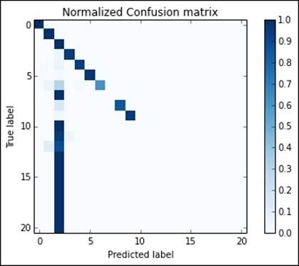
Manual tuning
Although the F1 score was close to 0.97, the normalized confusion matrix shows that the classes are strongly unbalanced and the classifier has just learned how to classify the most popular ones properly. To improve the results, we can resample each class, trying to balance the training dataset better.
First, let's count how many cases there are in the training dataset for each class:
In:
train_composition = train_df.groupBy("target").count().rdd.collectAsMap()
train_composition
Out:
{u'back': 2203,
u'buffer_overflow': 30,
u'ftp_write': 8,
u'guess_passwd': 53,
u'neptune': 107201,
u'nmap': 231,
u'normal': 97278,
u'perl': 3,
...
...
u'warezmaster': 20}
This is clear evidence of a strong imbalance. We can try to improve the performance by oversampling rare classes and subsampling too popular classes.
In this example, we will create a training dataset, where each class is represented at least 1,000 times, but up to 25,000. For this, let's first create the subsampling/oversampling rate and broadcast it throughout the cluster, and then flatMap each line of the training dataset to resample it properly:
In:
def set_sample_rate_between_vals(cnt, the_min, the_max):
if the_min <= cnt <= the_max:
# no sampling
return 1
elif cnt < the_min:
# Oversampling: return many times the same observation
return the_min/float(cnt)
else:
# Subsampling: sometime don't return it
return the_max/float(cnt)
sample_rates = {k:set_sample_rate_between_vals(v, 1000, 25000)
for k,v in train_composition.iteritems()}
sample_rates
Out:{u'back': 1,
u'buffer_overflow': 33.333333333333336,
u'ftp_write': 125.0,
u'guess_passwd': 18.867924528301888,
u'neptune': 0.23320677978750198,
u'nmap': 4.329004329004329,
u'normal': 0.2569954152017928,
u'perl': 333.3333333333333,
...
...
u'warezmaster': 50.0}
In:bc_sample_rates = sc.broadcast(sample_rates)
def map_and_sample(el, rates):
rate = rates.value[el['target']]
if rate > 1:
return [el]*int(rate)
else:
import random
return [el] if random.random() < rate else []
sampled_train_df = (train_df
.flatMap(
lambda x: map_and_sample(x, bc_sample_rates))
.toDF()
.cache())
The resampled dataset in the sampled_train_df DataFrame variable is also cached; we will use it many times during the hyperparameter optimization step. It should easily fit in-memory as the number of lines is lower than the original one:
In:sampled_train_df.count()
Out:97335
To get an idea of what's inside, we can print the first line. Pretty quick to print the value, isn't it? Of course, it's cached!
In:sampled_train_df.first()
Out:Row(duration=0.0, protocol_type=u'tcp', service=u'http', flag=u'SF', src_bytes=217.0, dst_bytes=2032.0, land=0.0, wrong_fragment=0.0, urgent=0.0, hot=0.0, num_failed_logins=0.0, logged_in=1.0, num_compromised=0.0, root_shell=0.0, su_attempted=0.0, num_root=0.0, num_file_creations=0.0, num_shells=0.0, num_access_files=0.0, num_outbound_cmds=0.0, is_host_login=0.0, is_guest_login=0.0, count=6.0, srv_count=6.0, serror_rate=0.0, srv_serror_rate=0.0, rerror_rate=0.0, srv_rerror_rate=0.0, same_srv_rate=1.0, diff_srv_rate=0.0, srv_diff_host_rate=0.0, dst_host_count=49.0, dst_host_srv_count=49.0, dst_host_same_srv_rate=1.0, dst_host_diff_srv_rate=0.0, dst_host_same_src_port_rate=0.02, dst_host_srv_diff_host_rate=0.0, dst_host_serror_rate=0.0, dst_host_srv_serror_rate=0.0, dst_host_rerror_rate=0.0, dst_host_srv_rerror_rate=0.0, target=u'normal')
Let's now use the pipeline that we created to make some predictions and print the F1 score of this new solution:
In:full_model = full_pipeline.fit(sampled_train_df)
predictions = full_model.transform(test_df)
print "F1-score test set:", evaluator.evaluate(predictions)
Out:F1-score test set: 0.967413322985
Test it on a classifier of 50 trees. To do so, we can build another pipeline (named refined_pipeline) and substitute the final stage with the new classifier. Performances seem the same even if the training set has been slashed in size:
In:clf = RandomForestClassifier(
numTrees=50, maxBins=100, seed=101,
labelCol="target_cat", featuresCol="features")
stages = full_pipeline.getStages()[:-1]
stages.append(clf)
refined_pipeline = Pipeline(stages=stages)
refined_model = refined_pipeline.fit(sampled_train_df)
predictions = refined_model.transform(test_df)
print "F1-score test set:", evaluator.evaluate(predictions)
Out:F1-score test set: 0.969943901769
Cross-validation
We can go forward with manual optimization and find the right model after having exhaustively tried many different configurations. Doing that, it would lead to both an immense waste of time (and reusability of the code) and will overfit the test dataset. Cross-validation is instead the correct key to run the hyperparameter optimization. Let's now see how Spark performs this crucial task.
First of all, as the training will be used many times, we can cache it. Let's therefore cache it after all the transformations:
In:pipeline_to_clf = Pipeline(
stages=preproc_stages + [assembler]).fit(sampled_train_df)
train = pipeline_to_clf.transform(sampled_train_df).cache()
test = pipeline_to_clf.transform(test_df)
The useful classes for hyperparameter optimization with-cross validation are contained in the pyspark.ml.tuning package. Two elements are essential: a grid map of parameters (that can be built with ParamGridBuilder) and the actual cross-validation procedure (run by the CrossValidator class).
In the example, we want to set some parameters of our classifier that won't change throughout the cross-validation. Exactly as with Scikit-learn, they're set when the classification object is created (in this case, column names, seed, and maximum number of bins).
Then, thanks to the grid builder, we decide which arguments should be changed for each iteration of the cross-validation algorithm. In the example, we want to check the classification performance changing the maximum depth of each tree in the forest from 3 to 12 (incrementing by 3) and the number of trees in the forest to 20 or 50.
Finally, we launch the cross-validation (with the fit method) after having set the grid map, classifier that we want to test, and number of folds. The parameter evaluator is essential: it will tell us which is the best model to keep after the cross-validation. Note that this operation may take 15-20 minutes to run (under the hood, 4*2*3=24 models are trained and tested):
In:
from pyspark.ml.tuning import ParamGridBuilder, CrossValidator
rf = RandomForestClassifier(
cacheNodeIds=True, seed=101, labelCol="target_cat",
featuresCol="features", maxBins=100)
grid = (ParamGridBuilder()
.addGrid(rf.maxDepth, [3, 6, 9, 12])
.addGrid(rf.numTrees, [20, 50])
.build())
cv = CrossValidator(
estimator=rf, estimatorParamMaps=grid,
evaluator=evaluator, numFolds=3)
cvModel = cv.fit(train)
Finally, we can predict the label using the cross-validated model as we're using a pipeline or classifier by itself. In this case, the performances of the classifier chosen with cross-validation are slightly better than in the previous case and allow us to beat the 0.97 barrier:
In:predictions = cvModel.transform(test)
print "F1-score test set:", evaluator.evaluate(predictions)
Out:F1-score test set: 0.97058134007
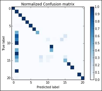
Furthermore, by plotting the normalized confusion matrix, you immediately realize that this solution is able to discover a wider variety of attacks, even the less popular ones:
In:metrics = MulticlassMetrics(predictions.select(
"prediction", "target_cat").rdd)
conf_matrix = metrics.confusionMa().toArray()
plot_confusion_matrix(conf_matrix)
Out:
Final cleanup
Here, we are at the end of the classification task. Remember to remove all the variables that you've used and the temporary table that you've created from the cache:
In:bc_sample_rates.unpersist()
sampled_train_df.unpersist()
train.unpersist()
After the Spark memory is cleared, we can turn off the Notebook.
Summary
This is the final chapter of the book. We have seen how to do data science at scale on a cluster of machines. Spark is able to train and test machine learning algorithms using all the nodes in a cluster with a simple interface, very similar to Scikit-learn. It's proved that this solution is able to cope with petabytes of information, creating a valid alternative to observation subsampling and online learning.
To become an expert in Spark and streaming processing, we strongly advise you to read the book, Mastering Apache Spark, Mike Frampton, Packt Publishing.
If you're brave enough to switch to Scala, the main programming language for Spark, this book is the best for such a transition: Scala for Data Science, Pascal Bugnion, Packt Publishing.
All materials on the site are licensed Creative Commons Attribution-Sharealike 3.0 Unported CC BY-SA 3.0 & GNU Free Documentation License (GFDL)
If you are the copyright holder of any material contained on our site and intend to remove it, please contact our site administrator for approval.
© 2016-2026 All site design rights belong to S.Y.A.