Large Scale Machine Learning with Python (2016)

Chapter 2. Scalable Learning in Scikit-learn

Loading a dataset into memory, preparing a data matrix, training a machine learning algorithm, and testing its generalization capabilities using out-of-sample observations are often not such a big deal given the quite powerful and yet affordable computers of this day and age. However, more and more frequently, the scale of the data to be elaborated is so huge that loading it into the core memory of your computer is not possible and, even if manageable, the result is intractable both in terms of data management and machine learning.

Alternative viable strategies beyond the core memory processing are possible: splitting the data into samples, using parallelism, and finally learning in small batches or by single instances. The present chapter will focus on the out-of-the-box solution that the Scikit-learn package offers: the streaming of mini batches of instances (our observations) from data storage and the incremental learning based on them. Such a solution is called out-of-core learning.

To treat the data by working on manageable chunks and learning incrementally is a great idea. However, when you try to implement it, it can also prove challenging because of the limitations in the available learning algorithms and streaming data in a flow will require you to think differently in terms of data management and feature extraction. Beyond presenting the Scikit-learn functionalities for out-of-core learning, we will also strive to present you with Python solutions for apparently daunting problems you can face when forced to observe only small portions of your data at a time.

In this chapter, we will cover the following topics:

· The way out-of-core learning is implemented in Scikit-learn

· Effectively managing streams of data using the hashing trick

· The nuts and bolts of stochastic learning

· Implementing data science with online learning

· Unsupervised transformations of streams of data

Out-of-core learning

Out-of-core learning refers to a set of algorithms working with data that cannot fit into the memory of a single computer, but that can easily fit into some data storage such as a local hard disk or web repository. Your available RAM, the core memory on your single machine, may indeed range from a few gigabytes (sometimes 2 GB, more commonly 4 GB, but we assume that you have 2 GB at maximum) up to 256 GB on large server machines. Large servers are like the ones you can get on cloud computing services such as Amazon Elastic Compute Cloud (EC2), whereas your storage capabilities can easily exceed terabytes of capacity using just an external drive (most likely about 1 TB but it can reach up to 4 TB).

As machine learning is based on globally reducing a cost function, many algorithms initially have been thought to work using all the available data and having access to it at each iteration of the optimization process. This is particularly true for all algorithms based on statistical learning that exploit matrix calculus, for instance, inverting matrices, but also algorithms based on greedy search need to have an evaluation on as much data as is possible before taking the next step. Therefore, the most common out-of-the-box regression-like algorithms (weighted linear combinations of features) update their coefficients trying to minimize the pooled error of the entire dataset. In a similar way, being so sensible to the noise present in the dataset, decision trees have to decide on the best splits based on all the data available in order to find an optimum solution.

If data cannot fit in the core memory of the computer in such a situation, you don't have many possible solutions. You can increase the available memory (depending on the limitations of the motherboard; after that, you will have to turn to distributed systems such as Hadoop and Spark, a solution we'll mention in the last chapters of the book) or simply reduce your dataset in order to have it fit the memory.

If your data is sparse, that is, you have many zero values in your dataset, you can transform your dense matrix into a sparse one. This is typical with textual data with many columns because each one is a word but with few values representing word counts because single documents usually display a limited selection of words. Sometimes, using sparse matrices can solve the problem allowing you to both load and process other quite large datasets, but this not a panacea (sorry, no free lunch, that is, there is no solution that can fit all problems) because some data matrices, though sparse, can have daunting sizes.

In such a situation, you can always try to reduce your dataset by cutting the number of instances or limiting the number of features, thus reducing the dimensions of the dataset matrix and its occupied area in-memory. Reducing the size of the dataset, by picking only a part of the observations, is a solution called subsampling (or simply sampling). Subsampling is not wrong per se but it has serious drawbacks and it is necessary to keep them in mind before deciding the course of analysis.

Subsampling as a viable option

When you subsample, you are actually discarding part of your informational richness and you cannot be so sure that you are only discarding redundant, not so useful observations. Actually, some hidden gems can be found only by considering all the data. Though computationally appealing—because subsampling just requires a random generator to tell you if you should pick an instance or not—by picking a subsampled dataset, you really risk limiting the capabilities of your algorithm to learn the rules and associations in your data in a complete way. In the bias-variance tradeoff, subsampling causes variance inflation of the predictions because estimates will be more uncertain due to random noise or outlying observations in your data.

In a world of big data, the algorithm with more quality data wins because it can learn more ways to relate predictions to predictors than other models with less (or more noisy) data. Consequently, subsampling, though acceptable as a solution, can impose a limit on the results of your machine learning activities because of less precise predictions and more variance of the estimates.

Subsampling limitations can be somehow overcome by learning multiple models on multiple subsamples of the data and then finally ensembling all the solutions or stacking the results of all the models together, thus creating a reduced data matrix for further training. This procedure is known as Bagging. (You actually compress the features in this way, thus reducing the space of your data in memory.) We will explore ensembling and stacking in a later chapter and discover how they can actually reduce the variance of estimates inflated by subsampling.

As an alternative, instead of cutting the instances, we could cut the features, but again, we will incur the problem that we need to build a model from the data in order to test what features we can select, so we still have to build a model with data that cannot fit in-memory.

Optimizing one instance at a time

Having realized that subsampling, though always viable, is not an optimal solution, we have to evaluate a different approach and out-of-core actually doesn't require you to give up observations or features. It just takes a bit longer to train a model, requiring more iterations and data transfer from your storage to your computer memory. We immediately provide a first intuition of how an out-of-core learning process works.

Let's start from the learning, which is a process where we try to map the unknown function expressing a response (a number or outcome that is a regression or classification problem) with respect to the available data. Learning is possible by fitting the internal coefficients of the learning algorithm trying to achieve the best fit on the data available that is minimizing a cost function, a measure that tells us how good our approximation is. Boiled down to basics, we are talking of an optimization process.

Different optimization algorithms, just like gradient descent, are processes able to work on any volume of data. They work at deriving a gradient for optimization (a direction in the optimization process) and they have the learning algorithm adapt its parameters in order to follow the gradient.

In the specific case of gradient descent, after a certain number of iterations, if the problem can be solved and there are no other problems such as a too high learning rate, the gradient should become so small that we can stop the optimization process. At the end of the process, we can be confident to have found a solution that is the optimum one (because it is a global optimum though sometimes it may be a local minimum, if the function to approximate is not convex).

As the directionality, dictated by the gradient, can be taken based on any volume of examples, it can also be taken on a single instance. Taking the gradient on a single instance requires a small learning rate, but in the end, the process can arrive at the same optimization as a gradient descent taken on the full data. In the end, all our algorithm needs is a direction to orientate correctly the learning process on its fitting the data available. Learning such a direction from a single case randomly taken from the data is therefore perfectly doable:

· We can obtain the same results as if we were working on all our data at one time, though the optimization path may turn a bit rough; if the majority of your observations point to an optimum direction, the algorithm will take that one. The only issue will be to correctly tune the correct parameters of the learning process and pass over the data multiple times in order to be sure for the optimization to complete as this learning procedure is much slower than working with all the data available.

· We don't have any particular issue in managing to keep a single instance in our core memory, leaving the bulk of the data out of it. Other issues may arise from moving the data by single examples from its repository to our core memory. Scalability is assured because the time it takes to process the data is linear; the time cost of using an instance more is always the same, no matter the total number of instances we have to process.

The approach of fitting a learning algorithm on a single instance or a subset of data fitting to memory at a time is called online learning and the gradient descent taken based on such single observations is called stochastic gradient descent. As previously suggested, online learning is an out-of-core technique and adopted by many learning algorithms in Scikit-learn.

Building an out-of-core learning system

We will illustrate the inner workings of a stochastic gradient descent in the next few paragraphs, offering more details and reasoning about it. Now knowing how it is possible to learn out-of-core (thanks to the stochastic gradient descent) allows us to depict with higher clarity what we should do to make it work on our computer.

You can partition your activity into different tasks:

1. Prepare your data repository access to stream the data instance by instance. This activity may require you to randomize the order of the data rows before fetching data to your computer in order to remove any information that ordering may bring about.

2. Do some data surveying first, maybe on a portion of all the data (for instance, the first ten thousand rows), trying to figure out if the arriving instances are consistent in their number of features, type of data, presence or lack of data values, minimum and maximum values for each variable, and mean and median. Find out the range or class of the target variable.

3. Prepare each received data row into a fixed format that can be accepted by the learning algorithm (a dense or sparse vector). At this stage, you can perform any basic transformation, turning categorical features into numeric ones, for instance, or having numeric features interact by themselves by a cross-product of the features themselves.

4. After randomizing the order of examples (as mentioned by the first point), establish a validation procedure using a systematic holdout or a holdout after a certain number of observations.

5. Tune hyperparameters by repeatedly streaming the data or working on small samples of it. This is also the right time to do some feature engineering (using unsupervised learning and special transformation functions such as kernel approximations) and leverage regularization and feature selection.

6. Build your final model using the data that you reserved for the training and ideally test the efficacy of the model on completely new data.

As a first step, we will discuss how to prepare your data and then easily create a stream suitable for online learning, leveraging useful functions from Python packages such as pandas and Scikit-learn.

Streaming data from sources

Some data is really streaming through your computer when you have a generative process that transmits data, which you can process on the fly or just discard, but not recall afterward unless you have stored it away in some data archival repository somewhere. It is like dragging water from a flowing river—the river keeps on flowing but you can filter and process all the water as it goes. It's a completely different strategy from processing all the data at once, which is more like putting all the water in a dam (an analogy for working with all the data in-memory).

As an example of streaming, we could quote the data flow produced instant by instant by a sensor or, even more simply, a Twitter streamline of tweets. Generally, the main sources of data streams are as follows:

· Environment sensors measuring temperature, pressure, and humidity

· GPS tracking sensors recording the location (latitude/longitude)

· Satellites recording image data

· Surveillance videos and sound records

· Web traffic

However, you won't often work on real streams of data but on static records left stored in a repository or file. In such cases, a stream can be recreated according to certain criteria, for example, extracting sequentially or randomly a single record at a time. If, for instance, our data is contained in a TXT or CSV file, all we need to do is fetch a single row of the file at a time and pass it to the learning algorithm.

For the examples in the present and following chapter, we will be working on files stored on your local hard disk and prepare the Python code necessary for its extraction as a stream. We won't use a toy dataset but we won't clutter your local hard drive with too much data for tests and demonstrations.

Datasets to try the real thing yourself

Since 1987, at University of California, Irvine (UCI), the UCI Machine Learning Repository has been hosted, which is a large repository of datasets for the empirical testing of machine learning algorithms by the machine learning community. At the time of writing this, the repository contains about 350 datasets from very different domains and purposes, from supervised regression and classification to unsupervised tasks. You can have a look at the available dataset at https://archive.ics.uci.edu/ml/.

From our side, we have selected a few datasets that will turn useful throughout the book, proposing challenging problems to you with an unusual, but still manageable, 2 GB RAM computer and a high number of rows or columns:

In order to download and use the dataset from the UCI repository, you have to go to the page dedicated to the dataset and follow the link under the title: Download: Data Folder. We have prepared some scripts for automatic downloading of the data that will be placed exactly in the directory that you are working with in Python, thus rendering the data access easier.

Here are some functions that we have prepared and will recall throughout the chapters when we need to download any of the datasets from UCI:

In: import urllib2 # import urllib.request as urllib2 in Python3

import requests, io, os, StringIO

import numpy as np

import tarfile, zipfile, gzip

def unzip_from_UCI(UCI_url, dest=''):

"""

Downloads and unpacks datasets from UCI in zip format

"""

response = requests.get(UCI_url)

compressed_file = io.BytesIO(response.content)

z = zipfile.ZipFile(compressed_file)

print ('Extracting in %s' % os.getcwd()+'\\'+dest)

for name in z.namelist():

if '.csv' in name:

print ('\tunzipping %s' %name)

z.extract(name, path=os.getcwd()+'\\'+dest)

def gzip_from_UCI(UCI_url, dest=''):

"""

Downloads and unpacks datasets from UCI in gzip format

"""

response = urllib2.urlopen(UCI_url)

compressed_file = io.BytesIO(response.read())

decompressed_file = gzip.GzipFile(fileobj=compressed_file)

filename = UCI_url.split('/')[-1][:-3]

with open(os.getcwd()+'\\'+filename, 'wb') as outfile:

outfile.write(decompressed_file.read())

print ('File %s decompressed' % filename)

def targzip_from_UCI(UCI_url, dest='.'):

"""

Downloads and unpacks datasets from UCI in tar.gz format

"""

response = urllib2.urlopen(UCI_url)

compressed_file = StringIO.StringIO(response.read())

tar = tarfile.open(mode="r:gz", fileobj = compressed_file)

tar.extractall(path=dest)

datasets = tar.getnames()

for dataset in datasets:

size = os.path.getsize(dest+'\\'+dataset)

print ('File %s is %i bytes' % (dataset,size))

tar.close()

def load_matrix(UCI_url):

"""

Downloads datasets from UCI in matrix form

"""

return np.loadtxt(urllib2.urlopen(UCI_url))

Tip

Downloading the example code

Detailed steps to download the code bundle are mentioned in the Preface of this book. Please have a look.

The code bundle for the book is also hosted on GitHub at https://github.com/PacktPublishing/Large-Scale-Machine-Learning-With-Python. We also have other code bundles from our rich catalog of books and videos available athttps://github.com/PacktPublishing/. Check them out!

The functions are just convenient wrappers built around various packages working with compressed data such as tarfile, zipfile, and gzip. The file is opened using the urllib2 module, which generates a handle to the remote system and allows the sequential transmission of data and being stored in memory as a string (StringIO) or in binary mode (BytesIO) from the io module—a module devoted to stream handling (https://docs.python.org/2/library/io.html). After being stored in memory, it is recalled just as a file would be from functions specialized in deflating the compressed files from disk.

The four provided functions should conveniently help you download the datasets quickly, no matter if they are zipped, tarred, gzipped, or just plain text in matrix form, avoiding the hassle of manual downloading and extraction operations.

The first example – streaming the bike-sharing dataset

As the first example, we will be working with the bike-sharing dataset. The dataset comprises of two CSV files containing the hourly and daily count of bikes rented in the years between 2011 and 2012 within the Capital Bike-share system in Washington D.C., USA. The data features the corresponding weather and seasonal information regarding the day of rental. The dataset is connected with a publication by Fanaee-T, Hadi, and Gama, Joao, Event labeling combining ensemble detectors and background knowledge, Progress in Artificial Intelligence (2013): pp. 1-15, Springer Berlin Heidelberg.

Our first target will be to save the dataset on the local hard disk using the convenient wrapper functions defined just a few paragraphs earlier:

In: UCI_url = 'https://archive.ics.uci.edu/ml/machine-learning-databases/00275/Bike-Sharing-Dataset.zip'

unzip_from_UCI(UCI_url, dest='bikesharing')

Out: Extracting in C:\scisoft\WinPython-64bit-2.7.9.4\notebooks\bikesharing

unzipping day.csv

unzipping hour.csv

If run successfully, the code will indicate in what directory the CSV files have been saved and print the names of both the unzipped files.

At this point, having saved the information on a physical device, we will write a script constituting the core of our out-of-core learning system, providing the data streaming from the file. We will first use the csv library, offering us a double choice: to recover the data as a list or Python dictionary. We will start with a list:

In: import os, csv

local_path = os.getcwd()

source = 'bikesharing\\hour.csv'

SEP = ',' # We define this for being able to easily change it as required by the file

with open(local_path+'\\'+source, 'rb') as R:

iterator = csv.reader(R, delimiter=SEP)

for n, row in enumerate(iterator):

if n==0:

header = row

else:

# DATA PROCESSING placeholder

# MACHINE LEARNING placeholder

pass

print ('Total rows: %i' % (n+1))

print ('Header: %s' % ', '.join(header))

print ('Sample values: %s' % ', '.join(row))

Out: Total rows: 17380

Header: instant, dteday, season, yr, mnth, hr, holiday, weekday, workingday, weathersit, temp, atemp, hum, windspeed, casual, registered, cnt

Sample values: 17379, 2012-12-31, 1, 1, 12, 23, 0, 1, 1, 1, 0.26, 0.2727, 0.65, 0.1343, 12, 37, 49

The output will report to us how many rows have been read, the content of the header—the first row of the CSV file (stored in a list)—and the content of a row (for convenience, we printed the last seen one). The csv.reader function creates an iterator that, thanks to a for loop, will release each row of the file one by one. Note that we have placed two remarks internally in the code snippet, pointing out where, throughout the chapter, we will place the other code to handle data preprocessing and machine learning.

Features in this case have to be handled using a positional approach, which is indexing the position of the label in the header. This can be a slight nuisance if you have to manipulate your features extensively. A solution could be to use csv.DictReader that produces a Python dictionary as an output (which is unordered but the features may be easily recalled by their labels):

In: with open(local_path+'\\'+source, 'rb') as R:

iterator = csv.DictReader(R, delimiter=SEP)

for n, row in enumerate(iterator):

# DATA PROCESSING placeholder

# MACHINE LEARNING placeholder

pass

print ('Total rows: %i' % (n+1))

print ('Sample values: %s' % str(row))

Out: Total rows: 17379

Sample values: {'mnth': '12', 'cnt': '49', 'holiday': '0', 'instant': '17379', 'temp': '0.26', 'dteday': '2012-12-31', 'hr': '23', 'season': '1', 'registered': '37', 'windspeed': '0.1343', 'atemp': '0.2727', 'workingday': '1', 'weathersit': '1', 'weekday': '1', 'hum': '0.65', 'yr': '1', 'casual': '12'}

Using pandas I/O tools

As an alternative to the csv module, we can use pandas' read_csv function. Such a function, specialized in uploading CSV files, is part of quite a large range of functions devoted to input/output on different file formats, as specified by the pandas documentation athttp://pandas.pydata.org/pandas-docs/stable/io.html.

The great advantages of using pandas I/O functions are as follows:

· You can keep your code consistent if you change your source type, that is, you need to redefine just the streaming iterator

· You can access a large number of different formats such as CSV, plain TXT, HDF, JSON, and SQL query for a specific database

· The data is streamed into chunks of the desired size as DataFrame data structures so that you can access the features in a positional way or by recalling their label, thanks to .loc, .iloc, .ix methods typical of slicing and dicing in a pandas dataframe

Here is an example using the same approach as before, this time built around pandas' read_csv function:

In: import pandas as pd

CHUNK_SIZE = 1000

with open(local_path+'\\'+source, 'rb') as R:

iterator = pd.read_csv(R, chunksize=CHUNK_SIZE)

for n, data_chunk in enumerate(iterator):

print ('Size of uploaded chunk: %i instances, %i features' % (data_chunk.shape))

# DATA PROCESSING placeholder

# MACHINE LEARNING placeholder

pass

print ('Sample values: \n%s' % str(data_chunk.iloc[0]))

Out:

Size of uploaded chunk: 2379 instances, 17 features

Size of uploaded chunk: 2379 instances, 17 features

Size of uploaded chunk: 2379 instances, 17 features

Size of uploaded chunk: 2379 instances, 17 features

Size of uploaded chunk: 2379 instances, 17 features

Size of uploaded chunk: 2379 instances, 17 features

Size of uploaded chunk: 2379 instances, 17 features

Sample values:

instant 15001

dteday 2012-09-22

season 3

yr 1

mnth 9

hr 5

holiday 0

weekday 6

workingday 0

weathersit 1

temp 0.56

atemp 0.5303

hum 0.83

windspeed 0.3284

casual 2

registered 15

cnt 17

Name: 0, dtype: object

Here, it is very important to notice that the iterator is instantiated by specifying a chunk size, that is, the number of rows the iterator has to return at every iteration. The chunksize parameter can assume values from 1 to any value, though clearly the size of the mini-batch (the chunk retrieved) is strictly connected to your available memory to store and manipulate it in the following preprocessing phase.

Bringing larger chunks into memory offers an advantage only in terms of disk access. Smaller chunks require multiple access to the disk and, depending on the characteristics of your physical storage, a longer time to pass through the data. Nevertheless, from a machine learning point of view, smaller or larger chunks make little difference for Scikit-learn out-of-core functions as they learn taking into account only one instance at a time, making them truly linear in computational cost.

Working with databases

As an example of the flexibility of the pandas I/O tools, we will provide a further example using a SQLite3 database where data is streamed from a simple query, chunk by chunk. The example is not proposed for just a didactical use. Working with a large data store in databases can indeed bring advantages from the disk space and processing time point of view.

Data arranged into tables in a SQL database can be normalized, thus removing redundancies and repetitions and saving disk storage. Database normalization is a way to arrange columns and tables in a database in a way to reduce their dimensions without losing any information. Often, this is accomplished by splitting tables and recoding repeated data into keys. Moreover, a relational database, being optimized on memory and operations and multiprocessing, can speed up and anticipate part of those preprocessing activities otherwise dealt within the Python scripting.

Using Python, SQLite (http://www.sqlite.org) is a good default choice because of the following reasons:

· It is open source

· It can handle large amounts of data (theoretically up to 140 TB per database, though it is unlikely to see any SQLite application dealing with such amounts of data)

· It operates on macOS and both Linux and Windows 32- and 64-bit environments

· It does not require any server infrastructure or particular installation (zero configuration) as all the data is stored in a single file on disk

· It can be easily extended using Python code to be turned into a stored procedure

Moreover, the Python standard library includes a sqlite3 module providing all the functions to create a database from scratch and work with it.

In our example, we will first upload the CSV file containing the bike-sharing dataset on both a daily and hourly basis to a SQLite database and then we will stream from it as we did from a CSV file. The database uploading code that we provide can be reusable throughout the book and for your own applications, not being tied to the specific example we provide (you just have to change the input and output parameters, that's all):

In : import os, sys

import sqlite3, csv,glob

SEP = ','

def define_field(s):

try:

int(s)

return 'integer'

except ValueError:

try:

float(s)

return 'real'

except:

return 'text'

def create_sqlite_db(db='database.sqlite', file_pattern=''):

conn = sqlite3.connect(db)

conn.text_factory = str # allows utf-8 data to be stored

c = conn.cursor()

# traverse the directory and process each .csv file useful for building the db

target_files = glob.glob(file_pattern)

print ('Creating %i table(s) into %s from file(s): %s' % (len(target_files), db, ', '.join(target_files)))

for k,csvfile in enumerate(target_files):

# remove the path and extension and use what's left as a table name

tablename = os.path.splitext(os.path.basename(csvfile))[0]

with open(csvfile, "rb") as f:

reader = csv.reader(f, delimiter=SEP)

f.seek(0)

for n,row in enumerate(reader):

if n==11:

types = map(define_field,row)

else:

if n>11:

break

f.seek(0)

for n,row in enumerate(reader):

if n==0:

sql = "DROP TABLE IF EXISTS %s" % tablename

c.execute(sql)

sql = "CREATE TABLE %s (%s)" % (tablename,\

", ".join([ "%s %s" % (col, ct) \

for col, ct in zip(row, types)]))

print ('%i) %s' % (k+1,sql))

c.execute(sql)

# Creating indexes for faster joins on long strings

for column in row:

if column.endswith("_ID_hash"):

index = "%s__%s" % \

( tablename, column )

sql = "CREATE INDEX %s on %s (%s)" % \

( index, tablename, column )

c.execute(sql)

insertsql = "INSERT INTO %s VALUES (%s)" % (tablename,

", ".join([ "?" for column in row ]))

rowlen = len(row)

else:

# raise an error if there are rows that don't have the right number of fields

if len(row) == rowlen:

c.execute(insertsql, row)

else:

print ('Error at line %i in file %s') % (n,csvfile)

raise ValueError('Houston, we\'ve had a problem at row %i' % n)

conn.commit()

print ('* Inserted %i rows' % n)

c.close()

conn.close()

The script provides a valid database name and pattern to locate the files that you want to import (wildcards such as * are accepted) and creates from scratch a new database and table that you need, filling them afterwards with all the data available:

In: create_sqlite_db(db='bikesharing.sqlite', file_pattern='bikesharing\\*.csv')

Out: Creating 2 table(s) into bikesharing.sqlite from file(s): bikesharing\day.csv, bikesharing\hour.csv

1) CREATE TABLE day (instant integer, dteday text, season integer, yr integer, mnth integer, holiday integer, weekday integer, workingday integer, weathersit integer, temp real, atemp real, hum real, windspeed real, casual integer, registered integer, cnt integer)

* Inserted 731 rows

2) CREATE TABLE hour (instant integer, dteday text, season integer, yr integer, mnth integer, hr integer, holiday integer, weekday integer, workingday integer, weathersit integer, temp real, atemp real, hum real, windspeed real, casual integer, registered integer, cnt integer)

* Inserted 17379 rows

The script also reports the data types for the created fields and number of rows, so it is quite easy to verify that everything has gone smoothly during the importation. Now it is easy to stream from the database. In our example, we will create an inner join between the hour and day tables and extract data on an hourly base with information about the total rentals of the day:

In: import os, sqlite3

import pandas as pd

DB_NAME = 'bikesharing.sqlite'

DIR_PATH = os.getcwd()

CHUNK_SIZE = 2500

conn = sqlite3.connect(DIR_PATH+'\\'+DB_NAME)

conn.text_factory = str # allows utf-8 data to be stored

sql = "SELECT H.*, D.cnt AS day_cnt FROM hour AS H INNER JOIN day as D ON (H.dteday = D.dteday)"

DB_stream = pd.io.sql.read_sql(sql, conn, chunksize=CHUNK_SIZE)

for j,data_chunk in enumerate(DB_stream):

print ('Chunk %i -' % (j+1)),

print ('Size of uploaded chunk: %i instances, %i features' % (data_chunk.shape))

# DATA PROCESSING placeholder

# MACHINE LEARNING placeholder

Out:

Chunk 1 - Size of uploaded chunk: 2500 instances, 18 features

Chunk 2 - Size of uploaded chunk: 2500 instances, 18 features

Chunk 3 - Size of uploaded chunk: 2500 instances, 18 features

Chunk 4 - Size of uploaded chunk: 2500 instances, 18 features

Chunk 5 - Size of uploaded chunk: 2500 instances, 18 features

Chunk 6 - Size of uploaded chunk: 2500 instances, 18 features

Chunk 7 - Size of uploaded chunk: 2379 instances, 18 features

If you need to speed up the streaming, you just have to optimize the database, first of all building the right indexes for the relational query that you intend to use.

Tip

conn.text_factory = str is a very important part of the script; it allows UTF-8 data to be stored. If such a command is ignored, you may experience strange errors when inputting data.

Paying attention to the ordering of instances

As a concluding remark for the streaming data topic, we have to warn you about the fact that, when streaming, you are actually including hidden information in your learning process because of the order of the examples you are basing your learning on.

In fact, online learners optimize their parameters based on each instance that they evaluate. Each instance will lead the learner toward a certain direction in the optimization process. Globally, the learner should take the right optimization direction, given a large enough number of evaluated instances. However, if the learner is instead trained by biased observations (for instance, observations ordered by time or grouped in a meaningful way), the algorithm will also learn the bias. Something can be done during training in order to not remember previously seen instances, but some bias will be introduced anyway. If you are learning time series—the response to the flow of time often being part of the model—such a bias is quite useful, but in most other cases, it acts as some kind ofoverfitting and translates into a certain lack of generalization in the final model.

If your data has some kind of ordering which you don't want to be learned by the machine learning algorithm (such as an ID order), as a cautionary measure, you can shuffle its rows before streaming the data and obtain a random order more suitable for online stochastic learning.

The fastest way, and the one occupying less space on disk, is to stream the dataset in memory and shrink it by compression. In most cases, but not all, this will work thanks to the compression algorithm applied and the relative sparsity and redundancy of the data that you are using for the training. In the cases where it doesn't work, you have to shuffle the data directly on the disk implying more disk space consumption.

Here, we first present a fast way to shuffle in-memory, thanks to the zlib package that can rapidly compress the rows into memory, and the shuffle function from the random module:

In: import zlib

from random import shuffle

def ram_shuffle(filename_in, filename_out, header=True):

with open(filename_in, 'rb') as f:

zlines = [zlib.compress(line, 9) for line in f]

if header:

first_row = zlines.pop(0)

shuffle(zlines)

with open(filename_out, 'wb') as f:

if header:

f.write(zlib.decompress(first_row))

for zline in zlines:

f.write(zlib.decompress(zline))

import os

local_path = os.getcwd()

source = 'bikesharing\\hour.csv'

ram_shuffle(filename_in=local_path+'\\'+source, \

filename_out=local_path+'\\bikesharing\\shuffled_hour.csv', header=True)

Tip

For Unix users, the sort command, which can be easily used with a single invocation (the -R parameter), shuffles huge amounts of text files very easily and much more efficiently than any Python implementation. It can be combined with decompression and compression steps using pipes.

So something like the following command should do the trick:

zcat sorted.gz | sort -R | gzip - > shuffled.gz

In case the RAM is not enough to store all the compressed data, the only viable solution is to operate on the file as it is on the disk itself. The following snippet of code defines a function that will repeatedly split your file into increasingly smaller files, shuffle them internally, and arrange them again randomly in a larger file. The result is not a perfect random rearrangement, but the rows are scattered around enough to destroy any previous order that could influence online learning:

In: from random import shuffle

import pandas as pd

import numpy as np

import os

def disk_shuffle(filename_in, filename_out, header=True, iterations = 3, CHUNK_SIZE = 2500, SEP=','):

for i in range(iterations):

with open(filename_in, 'rb') as R:

iterator = pd.read_csv(R, chunksize=CHUNK_SIZE)

for n, df in enumerate(iterator):

if n==0 and header:

header_cols =SEP.join(df.columns)+'\n'

df.iloc[np.random.permutation(len(df))].to_csv(str(n)+'_chunk.csv', index=False, header=False, sep=SEP)

ordering = list(range(0,n+1))

shuffle(ordering)

with open(filename_out, 'wb') as W:

if header:

W.write(header_cols)

for f in ordering:

with open(str(f)+'_chunk.csv', 'r') as R:

for line in R:

W.write(line)

os.remove(str(f)+'_chunk.csv')

filename_in = filename_out

CHUNK_SIZE = int(CHUNK_SIZE / 2)

import os

local_path = os.getcwd()

source = 'bikesharing\\hour.csv'

disk_shuffle(filename_in=local_path+'\\'+source, \

filename_out=local_path+'\\bikesharing\\shuffled_hour.csv', header=True)

Stochastic learning

Having defined the streaming process, it is now time to glance at the learning process as it is the learning and its specific needs that determine the best way to handle data and transform it in the preprocessing phase.

Online learning, contrary to batch learning, works with a larger number of iterations and gets directions from each single instance at a time, thus allowing a more erratic learning procedure than an optimization made on a batch, which immediately tends to get the right direction expressed from the data as a whole.

Batch gradient descent

The core algorithm for machine learning, gradient descent, is therefore revisited in order to adapt to online learning. When working on batch data, gradient descent can minimize the cost function of a linear regression analysis using much less computations than statistical algorithms. The complexity of gradient descent ranks in the order O(n*p), making learning regression coefficients feasible even in the occurrence of a large n (which stands for the number of observations) and large p (number of variables). It also works perfectly when highly correlated or even identical features are present in the training data.

Everything is based on a simple optimization method: the set of parameters is changed through multiple iterations in a way that it gradually converges to the optimal solution starting from a random one. Gradient descent is a theoretically well-understood optimization method with known convergence guarantees for certain problems such as regression ones. Nevertheless, let's start with the following image representing a complex mapping (typical of neural networks) between the values that the parameters can take (representing the hypothesis space) and result in terms of minimization of the cost function:

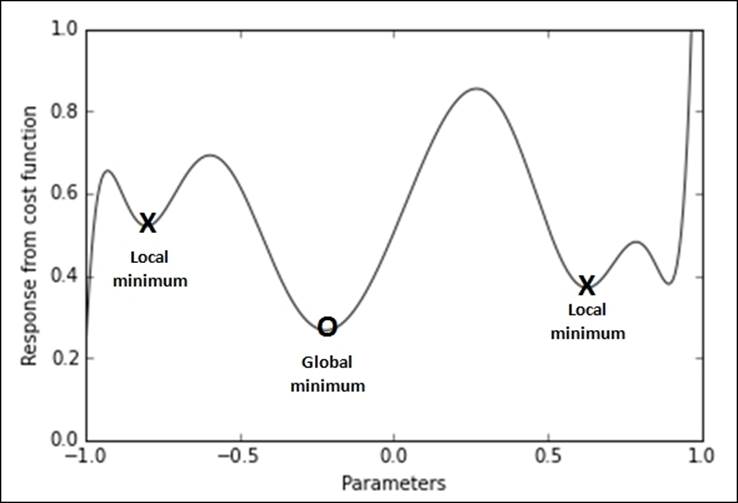
Using a figurative example, gradient descent resembles walking blindfolded around mountains. If you want to descend to the lowest valley without being able to see the path, you can just proceed by taking the direction that you feel is going downhill; try it for a while, then stop, feel the terrain again, and then proceed toward where you feel it is going downhill, and so on, again and again. If you keep on heading toward where the surface descends, you will finally arrive at a point when you cannot descend anymore because the terrain is flat. Hopefully, at that point, you should have reached your destination.

Using such a method, you need to perform the following actions:

· Decide the starting point. This is usually achieved by an initial random guess of the parameters of your function (multiple restarts will ensure that the initialization won't cause the algorithm to reach a local optimum because of an unlucky initial setting).

· Be able to feel the terrain, that is, be able to tell when it goes down. In mathematical terms, this means that you should be able to take the derivative of your actual parameterized function with respect to your target variable, that is, the partial derivative of the cost function that you are optimizing. Note that the gradient descent works on all of your data, trying to optimize the predictions from all your instances at once.

· Decide how long you should follow the direction dictated by the derivative. In mathematical terms, this corresponds to a weight (usually called alpha) to decide how much you should change your parameters at every step of the optimization. This aspect can be considered as the learning factor because it points out how much you should learn from the data at each optimization step. As with any other hyperparameter, the best value of alpha can be determined by performance evaluation on a validation set.

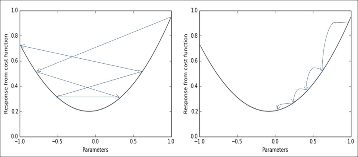
· Determine when to stop, given a too marginal improvement of the cost function with respect to the previous step. In such a sense, you also should be able to notice when something goes wrong and you are not going in the right direction maybe because you are using too large an alpha for the learning. This is actually a matter of momentum, that is, the speed at which the algorithm converges toward the optimum. It is just like throwing a ball down a mountainside: it just rolls over small dents in the surface, but if its speed is too high, it won't stop at the right point. Thus, if alpha is set correctly, the momentum will naturally slow down as the algorithm is approaching the optimum as shown in the following image in the right panel. However, if it is not set properly, it will just jump over the global optimum and report further errors to be minimized, as depicted in the following image on the right panel, when the optimization process causes parameters to jump across different values without achieving the required error minimization:

In order to better depict what happens with gradient descent, let's take the example of a linear regression whose parameters are optimized by such a procedure.

We start from the cost function J given the vector of weights w:

The matrix-vector multiplication Xw between the training data matrix X and the vector of coefficients w represents the predictions from the linear model, whose deviance from the response y is squared, then summed, and finally divided by two times n, the number of instances.

Initially, the vector w could be instantiated using random numbers taken from the standardized normal distribution whose mean is zero and standard deviation is the unit. (Actually, initialization can be done in a lot of different ways, all working equally well to approximate linear regression whose cost function is bowl-shaped and has a unique minimum.) This allows our algorithm to start somewhere along the optimization path and could effectively speed up the convergence of the process. As we are optimizing a linear regression, initialization shouldn't cause much trouble to the algorithm (at worst, a wrong start will just slow it down). Instead, when we are using gradient descent in order to optimize different machine learning algorithms such as neural networks, we risk being stuck because of a wrong initialization. This will happen if, for instance, the initial w is just filled with zero values (the risk is getting stuck on a perfectly symmetric hilltop, where no directionality can immediately bring an optimization better than any other). This can happen with optimization processes that have multiple local minima, too.

Given the starting random coefficients vector w, we can immediately calculate the cost function J(w) and determine the initial direction for each single coefficient by subtracting from each a portion alpha (α, the learning rate) of the partial derivative of the cost function, as explicated by the following formula:

This can be better conveyed after solving the partial derivative, as follows:

Noticeably, the update is done on each singular coefficient (wj) given its feature vector xj, but based on all the predictions at once (hence the summation).

After iterating over all the coefficients in w, the coefficients' update will be completed and the optimization may restart again by calculating the partial derivative and updating the w vector.

An interesting characteristic of the process is that the update will be less and less as the w vector approaches the optimal configuration. Therefore, the process could stop when the change induced in w, with respect to the previous operation, is small. Anyway, it is true that we have decreasing updates when alpha, the learning rate, is set to the right size. In fact, if its value is too large, it may cause the optimization to detour and fail, causing—in some cases—a complete divergence of the process and the impossibility to converge finally to a solution. In fact, the optimization will tend to overshoot the target and actually get farther away from it.

At the other end, too small an alpha value will not only move the optimization process toward its target too slowly, but it may also be easily stuck somewhere in a local minima. This is especially true with regard to more complex algorithms, just like neural networks. As for linear regression and its classification counterpart, logistic regression, because the optimization curve is bowl-shaped, just like a concave curve, it features a single minimum and no local minima at all.

In the implementation that we illustrated, alpha is a fixed constant (a fixed learning rate gradient descent). As alpha plays such an important role in converging to an optimal solution, different strategies have been devised for it to start larger and shrink as the optimization goes on. We will discuss such different approaches when examining the Scikit-learn implementation.

Stochastic gradient descent

The version of the gradient descent seen so far is known as full batch gradient descent and works by optimizing the error of the entire dataset, and thus needs it in-memory. The out-of-core versions are the stochastic gradient descent (SGD) and mini batch gradient descent.

Here, the formulation stays exactly the same, but for the update; the update is done for a single instance at a time, thus allowing us to leave the core data in its storage and take just a single observation in-memory:

The core idea is that, if the instances are picked randomly without particular biases, the optimization will move on average toward the target cost minimization. That explains why we discussed how to remove any ordering from a stream and making it as random as possible. For instance, in the bike-sharing example, if you have stochastic gradient descent learn the patterns of the early season first, then focus on the summer, then on the fall, and so on, depending on the season when the optimization is stopped, the model will be tuned to predict one season better than the others because most of the recent examples are from that season. In a stochastic gradient descent optimization, when data is independent and identically distributed (i.i.d.), convergence to the global minimum is guaranteed. Practically, i.i.d. means that your examples should have no sequential order or distribution but should be proposed to the algorithm as if picked randomly from your available ones.

The Scikit-learn SGD implementation

A good number of online learning algorithms can be found in the Scikit-learn package. Not all machine learning algorithms have an online counterpart, but the list is interesting and steadily growing. As for supervised learning, we can divide available learners into classifiers and regressors and enumerate them.

As classifiers, we can mention the following:

· sklearn.naive_bayes.MultinomialNB

· sklearn.naive_bayes.BernoulliNB

· sklearn.linear_model.Perceptron

· sklearn.linear_model.PassiveAggressiveClassifier

· sklearn.linear_model.SGDClassifier

As regressors, we have two options:

· sklearn.linear_model.PassiveAggressiveRegressor

· sklearn.linear_model.SGDRegressor

They all can learn incrementally, updating themselves instance by instance; though only SGDClassifier and SGDRegressor are based on the stochastic gradient descent optimization that we previously described, and they are the main topics of this chapter. The SGD learners are optimal for all large-scale problems as their complexity is bound to O(k*n*p), where k is the number of passes over the data, n is the number of instances, and p is the number of features (naturally non-zero features if we are working with sparse matrices): a perfectly linear time learner, taking more time exactly in proportion to the number of examples shown.

Other online algorithms will be used as a comparative benchmark. Moreover, all algorithms have the usage of the same API in common, based on the partial_fit method for online learning and mini-batch (when you stream larger chunks rather than a single instance). Sharing the same API makes all these learning techniques interchangeable in your learning frame.

Contrary to the fit method, which uses all the available data for its immediate optimization, partial_fit operates a partial optimization based on each of the single instances passed. Even if a dataset is passed to the partial_fit method, the algorithm won't process the entire batch but for its single elements, making the complexity of the learning operations indeed linear. Moreover, a learner, after partial_fit, can be perpetually updated by subsequent partial_fit calls, making it perfect for online learning from continuous streams of data.

When classifying, the only caveat is that at the first initialization, it is necessary to know how many classes we are going to learn and how they are labeled. This can be done using the classes parameter, pointing out a list of the numeric values labels. This requires to be explored beforehand, streaming through the data in order to record the labels of the problem and also taking notice of their distribution in case they are unbalanced—a class is numerically too large or too small with respect to the others (but the Scikit-learn implementation offers a way to automatically handle the problem). If the target variable is numeric, it is still useful to know its distribution, but this is not necessary to successfully run the learner.

In Scikit-learn, we have two implementations—one for classification problems (SGDClassifier) and one for regression ones (SGDRegressor). The classification implementation can handle multiclass problems using the one-vs-all (OVA) strategy. This strategy implies that, given k classes, k models are built, one for each class against all the instances of other classes, therefore creating k binary classifications. This will produce k sets of coefficients and k vectors of predictions and their probability. In the end, based on the emitted probability of each class compared against the other, the classification is assigned to the class with the highest probability. If we need to give actual probabilities for the multinomial distribution, we can simply normalize the results by dividing by their sum. (This is what is happening in a softmax layer in a neural network, which we will see in the following chapters.)

Both classification and regression SGD implementations in Scikit-learn feature different loss functions (the cost function, the core of the stochastic gradient descent optimization).

For classification, expressed by the loss parameter, we can rely on the following:

· loss='log': Classical logistic regression

· loss='hinge': Softmargin, that is, a linear support vector machine

· loss='modified_huber': A smoothed hinge loss

For regression, we have three loss functions:

· loss='squared_loss': Ordinary least squares (OLS) for linear regression

· loss='huber': Huber loss for robust regression against outliers

· loss='epsilon_insensitive': A linear support vector regression

We will present some examples using the classical statistical loss functions, which are logistic loss and OLS. Hinge loss and support vector machines (SVMs) will be discussed in the next chapter, a detailed introduction about their functioning being necessary.

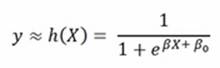
As a reminder (so that you won't have to go and consult any other supplementary machine learning book), if we define the regression function as h and its predictions are given by h(X) because X is the matrix of features, then the following is the suitable formulation:

Consequently, the OLS cost function to be minimized is as follows:

In logistic regression, having a transformation of the binary outcome 0/1 into an odds ratio, πy being the probability of a positive outcome, the formula is as follows:

The logistic cost function, consequently, is defined as follows:

Defining SGD learning parameters

To define SGD parameters in Scikit-learn, both in classification and regression problems (so that they are valid for both SGDClassifier and SGDRegressor), we have to make clear how to deal with some important parameters necessary for a correct learning when you cannot evaluate all the data at once.

The first one is n_iter, which defines the number of iterations through the data. Initially set to 5, it has been empirically shown that it should be tuned in order for the learner, given the other default parameters, to see around 10^6 examples; therefore a good solution to set it would be n_iter = np.ceil(10**6 / n), where n is the number of instances. Noticeably, n_iter only works with in-memory datasets, so it acts only when you operate by the fit method but not with partial_fit. In reality, partial_fit will reiterate over the same data just if you restream it in your procedure and the right number of iterations of restreams is something to be tested along the learning procedure itself, being influenced by the type of data. In the next chapter, we will illustrate hyperparameter optimization and the right number of passes will be discussed.

Tip

It might make sense to reshuffle the data after each complete pass over all of the data when doing mini-batch learning.

shuffle is a parameter required if you want to shuffle your data. It refers to the mini-batch present in-memory and not to out-of-core data ordering. It also works with partial_fit but its effect in such a case is very limited. Always set it to True, but for data to be passed in chunks, shuffle your data out-of-core, as we described before.

warm_start is another parameter that works with the fit method because it remembers the previous fit coefficients (but not the learning rate if it has been dynamically modified). If you are using the partial_fit method, the algorithm will remember the previouslylearned coefficients and the state of the learning rate schedule.

The average parameter triggers a computational trick that, at a certain instance, starts averaging new coefficients with older ones allowing a faster convergence. It can be set to True or an integer value indicating from what instance it will start averaging.

Last, but not least, we have learning_rate and its related parameters, eta0 and power_t. The learning_rate parameter implies how each observed instance impacts on the optimization process. When presenting SGD from a theoretical point of view, we presented constant rate learning, which can be replicated setting learning_rate='constant'.

However, other options are present, letting the eta (called the learning rate in Scikit-learn and defined at time t) gradually decrease. In classification, the solution proposed is learning_rate='optimal', given by the following formulation:

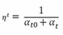
Here, t is the time steps, given by the number of instances multiplied by iterations, and t0 is a value heuristically chosen because of the studies by Léon Bottou, whose version of the Stochastic Gradient SVM has heavily influenced the SGD Scikit-learn implementation (http://leon.bottou.org/projects/sgd). The clear advantage of such a learning strategy is that learning decreases as more examples are seen, avoiding sudden perturbations of the optimization given by unusual values. Clearly, this strategy is also out-of-the-box, meaning that you don't have much to do with it.

In regression, the suggested learning fading is given by this formulation, corresponding to learning_rate= 'invscaling':

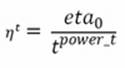
Here, eta0 and power_t are hyperparameters to be optimized by an optimization search (they are initially set to 0 and 0.5). Noticeably, using the invscaling learning rate, SGD will start with a lower learning rate, less than the optimal rate one, and it will decrease more slowly, being a bit more adaptable during learning.

Feature management with data streams

Data streams pose the problem that you cannot evaluate as you would do when working on a complete in-memory dataset. For a correct and optimal approach to feed your SGD out-of-core algorithm, you first have to survey the data (by taking a chuck of the initial instances of the file, for example) and find out the type of data you have at hand.

We distinguish among the following types of data:

· Quantitative values

· Categorical values encoded with integer numbers

· Unstructured categorical values expressed in textual form

When data is quantitative, it could just be fed to the SGD learner but for the fact that the algorithm is quite sensitive to feature scaling; that is, you have to bring all the quantitative features into the same range of values or the learning process won't converge easily and correctly. Possible scaling strategies are converting all the values in the range [0,1], [-1,1] or standardizing the variable by centering its mean to zero and converting its variance to the unit. We don't have particular suggestions for the choice of the scaling strategy, but converting in the range [0,1] works particularly well if you are dealing with a sparse matrix and most of your values are zero.

As for in-memory learning, when transforming variables on the training set, you have to take notice of the values that you used (Basically, you need to get minimum, maximum, mean, and standard deviation of each feature.) and reuse them in the test set in order to achieve consistent results.

Given the fact that you are streaming data and it isn't possible to upload all the data in-memory, you have to calculate them by passing through all the data or at least a part of it (sampling is always a viable solution). The situation of working with an ephemeral stream (a stream you cannot replicate) poses even more challenging problems; in fact, you have to constantly keep trace of the values that you keep on receiving.

If sampling just requires you to calculate your statistics on a chunk of n instances (under the assumption that your stream has no particular order), calculating statistics on the fly requires you to record the right measures.

For minimum and maximum, you need to store a variable each for every quantitative feature. Starting from the very first value, which you will store as your initial minimum and maximum, for each new value that you will receive from the stream you will have to confront it with the previously recorded minimum and maximum values. If the new instance is out of the previous range of values, you just update your variable accordingly.

In addition, the average doesn't pose any particular problems because you just need to keep a sum of the values seen and a count of the instances. As for variance, you need to recall that the textbook formulation is as follows:

Noticeably, you need to know the mean μ, which you are also just learning incrementally from the stream. However, the formulation can be explicated as follows:

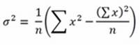
As you are just recording the number n of instances and a summation of x values, you just need to store another variable, which is the summation of values of x squared, and you will have all the ingredients for the recipe.

As an example, using the bike-sharing dataset, we can calculate the running mean, standard deviation, and range reporting the final result and plot how such stats changed as data was streamed from disk:

In: import os, csv

local_path = os.getcwd()

source = 'bikesharing\\hour.csv'

SEP=','

running_mean = list()

running_std = list()

with open(local_path+'\\'+source, 'rb') as R:

iterator = csv.DictReader(R, delimiter=SEP)

x = 0.0

x_squared = 0.0

for n, row in enumerate(iterator):

temp = float(row['temp'])

if n == 0:

max_x, min_x = temp, temp

else:

max_x, min_x = max(temp, max_x),min(temp, min_x)

x += temp

x_squared += temp**2

running_mean.append(x / (n+1))

running_std.append(((x_squared - (x**2)/(n+1))/(n+1))**0.5)

# DATA PROCESSING placeholder

# MACHINE LEARNING placeholder

pass

print ('Total rows: %i' % (n+1))

print ('Feature \'temp\': mean=%0.3f, max=%0.3f, min=%0.3f,\ sd=%0.3f' % (running_mean[-1], max_x, min_x, running_std[-1]))

Out: Total rows: 17379

Feature 'temp': mean=0.497, max=1.000, min=0.020, sd=0.193

In a few moments, the data will be streamed from the source and key figures relative to the temp feature will be recorded as a running estimation of the mean and standard deviation is calculated and stored in two separated lists.

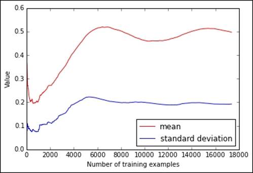
By plotting the values present in the lists, we can examine how much the estimates fluctuated with respect to the final figures and get an idea about how many instances are required before getting a stable mean and standard deviation estimate:

In: import matplotlib.pyplot as plt

%matplotlib inline

plt.plot(running_mean,'r-', label='mean')

plt.plot(running_std,'b-', label='standard deviation')

plt.ylim(0.0,0.6)

plt.xlabel('Number of training examples')

plt.ylabel('Value')

plt.legend(loc='lower right', numpoints= 1)

plt.show()

If you previously processed the original bike-sharing dataset, you will obtain a plot where clearly there is a trend in the data (due to temporal ordering, because the temperature naturally varies with seasons):

On the contrary, if we had used the shuffled version of the dataset as a source, the shuffled_hour.csv file, we could have obtained a couple of much more stable and quickly converging estimates. Consequently, we would have learned an approximate but more reliable estimate of the mean and standard deviation observing fewer instances from the stream:

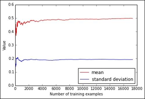
The difference in the two charts reminds us of the importance of randomizing the order of the observations. Even learning simple descriptive statistics can be influenced heavily by trends in the data; consequently, we have to pay more attention when learning complex models by SGD.

Describing the target

In addition, the target variable also needs to be explored before starting. We need, in fact, to be sure about what values it assumes, if categorical, and figure out if it is unbalanced when in classes or has a skewed distribution when a number.

If we are learning a numeric response, we can adopt the same strategy shown previously for the features, whereas for classes, a Python dictionary keeping a count of classes (the keys) and their frequencies (the values) will suffice.

As an example, we will download a dataset for classification, the Forest Covertype data.

For a fast download and preparation of the data, we will use the gzip_from_UCI function as defined in the Datasets to try the real thing yourself section of the present chapter:

In: UCI_url = 'https://archive.ics.uci.edu/ml/machine-learning-databases/covtype/covtype.data.gz'

gzip_from_UCI(UCI_url)

In case of problems in running the code, or if you prefer to prepare the file by yourself, just go to the UCI website, download the dataset, and unpack it on the directory where Python is currently working:

https://archive.ics.uci.edu/ml/machine-learning-databases/covtype/

Once the data is available on disk, we can scan through the 581,012 instances, converting the last value of each row, representative of the class that we should estimate, to its corresponding forest cover type:

In: import os, csv

local_path = os.getcwd()

source = 'covtype.data'

SEP=','

forest_type = {1:"Spruce/Fir", 2:"Lodgepole Pine", \

3:"Ponderosa Pine", 4:"Cottonwood/Willow",\

5:"Aspen", 6:"Douglas-fir", 7:"Krummholz"}

forest_type_count = {value:0 for value in forest_type.values()}

forest_type_count['Other'] = 0

lodgepole_pine = 0

spruce = 0

proportions = list()

with open(local_path+'\\'+source, 'rb') as R:

iterator = csv.reader(R, delimiter=SEP)

for n, row in enumerate(iterator):

response = int(row[-1]) # The response is the last value

try:

forest_type_count[forest_type[response]] +=1

if response == 1:

spruce += 1

elif response == 2:

lodgepole_pine +=1

if n % 10000 == 0:

proportions.append([spruce/float(n+1),\

lodgepole_pine/float(n+1)])

except:

forest_type_count['Other'] += 1

print ('Total rows: %i' % (n+1))

print ('Frequency of classes:')

for ftype, freq in sorted([(t,v) for t,v \

in forest_type_count.iteritems()], key = \

lambda x: x[1], reverse=True):

print ("%-18s: %6i %04.1f%%" % \

(ftype, freq, freq*100/float(n+1)))

Out: Total rows: 581012

Frequency of classes:

Lodgepole Pine : 283301 48.8%

Spruce/Fir : 211840 36.5%

Ponderosa Pine : 35754 06.2%

Krummholz : 20510 03.5%

Douglas-fir : 17367 03.0%

Aspen : 9493 01.6%

Cottonwood/Willow : 2747 00.5%

Other : 0 00.0%

The output displays that two classes, Lodgepole Pine and Spruce/Fir, account for most observations. If examples are shuffled appropriately in the stream, the SGD will appropriately learn the correct a-priori distribution and consequently adjust its probability emission (a-posteriori probability).

If, contrary to our present case, your objective is not classification accuracy but increasing the receiver operating characteristic (ROC) area under the curve (AUC) or f1-score (error functions that can be used for evaluation; for an overview, you can directly consult the Scikit-learn documentation at http://scikit-learn.org/stable/modules/model_evaluation.html regarding a classification model trained on imbalanced data, and then the provided information can help you balance the weights using the class_weight parameter when defining SGDClassifier or sample_weight when partially fitting the model. Both change the impact of the observed instance by overweighting or underweighting it. In both ways, operating these two parameters will change the a-priori distribution. Weighting classes and instances will be discussed in the next chapter.

Before proceeding to training and working with classes, we can check whether the proportion of classes is always consistent in order to convey the correct a-priori probability to the SGD:

import matplotlib.pyplot as plt

import numpy as np

%matplotlib inline

proportions = np.array(proportions)

plt.plot(proportions[:,0],'r-', label='Spruce/Fir')

plt.plot(proportions[:,1],'b-', label='Lodgepole Pine')

plt.ylim(0.0,0.8)

plt.xlabel('Training examples (unit=10000)')

plt.ylabel('%')

plt.legend(loc='lower right', numpoints= 1)

plt.show()

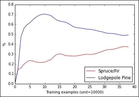
In the previous figure, you can notice how the percentage of examples change as we progress streaming the data in the existing order. A shuffle is really necessary, in this case, if we want a stochastic online algorithm to learn correctly from data.

Actually, the proportions are changeable; this dataset has some kind of ordering, maybe a geographic one, that should be corrected by shuffling the data or we will risk overestimating or underestimating certain classes with respect to others.

The hashing trick

If, among your features, there are categories (encoded in values or left in textual form), things can get a bit trickier. Normally, in batch learning, you would one-hot encode the categories and get as many new binary features as categories that you have. Unfortunately, in a stream, you do not know in advance how many categories you will deal with, and not even by sampling can you be sure of their number because rare categories may appear really late in the stream or require a too large sample to be discovered. You will have to first stream all the data and take a record of every category that appears. Anyway, streams can be ephemeral and sometimes the number of classes can be so large that they cannot be stored in-memory. The online advertising data is such an example because of its high volumes that are difficult to store away and because the stream cannot be passed over more than once. Moreover, advertising data is quite varied and features change constantly.

Working with texts makes the problem even more strikingly evident because you cannot anticipate what kind of word could be part of the text that you will be analyzing. In a bag-of-words model—where for each text the present words are counted and their frequency value pasted in an element in the feature vector specific to each word—you should be able to map each word to an index in advance. Even if you can manage this, you'll always have to handle the situation when an unknown word (therefore never mapped before) will pop up during testing or when the predictor is in production. Marginally, it should also be added that, being a spoken language, dictionaries made of hundreds of thousands or even millions of different terms are not unusual at all.

To recap, if you can handle knowing in advance the classes in your features, you can deal with them using the one-hot encoder from Scikit-learn (http://Scikit-learn.org/stable/modules/generated/sklearn.preprocessing.OneHotEncoder.html). We actually won't illustrate it here but basically the approach is not at all different from what you would apply when working with batch learning. What we want to illustrate to you is when you cannot really apply one-hot encoding.

There is a solution called the hashing trick because it is based on the hash function and can deal with both text and categorical variables in integer or string form. It can also work with categorical variables mixed with numeric values from quantitative features. The core problem with one-hot encoding is that it assigns a position to a value in the feature vector after having mapped its feature to that position. The hashing trick can univocally map a value to its position without any prior need to evaluate the feature because it leverages the core characteristic of a hashing function—to transform a value or string into an integer value deterministically.

Therefore, the only necessary preparation before applying it is creating a sparse vector large enough to represent the complexity of the data (potentially containing from 2**19 to 2**30 elements, depending on the available memory, bus architecture of your computer, and type of hash function that you are using). If you are working on some text, you'll also need a tokenizer, that is, a function that will split your text into single words and removes punctuation.

A simple toy example will make this clear. We will be using two specialized functions from the Scikit-learn package: HashingVectorizer, a transformer based on the hashing trick that works on textual data, and FeatureHasher, which is another transformer, specialized in converting a data row expressed as a Python dictionary to a sparse vector of features.

As the first example, we will turn a phrase into a vector:

In: from sklearn.feature_extraction.text import HashingVectorizer

h = HashingVectorizer(n_features=1000, binary=True, norm=None)

sparse_vector = h.transform(['A simple toy example will make clear how it works.'])

print(sparse_vector)

Out:

(0, 61) 1.0

(0, 271) 1.0

(0, 287) 1.0

(0, 452) 1.0

(0, 462) 1.0

(0, 539) 1.0

(0, 605) 1.0

(0, 726) 1.0

(0, 918) 1.0

The resulting vector has unit values only at certain indexes, pointing out an association between a token in the phrase (a word) and a certain position in the vector. Unfortunately, the association cannot be reversed unless we map the hash value for each token in an external Python dictionary. Though possible, such a mapping would be indeed memory consuming because dictionaries can prove large, in the range of millions of items or even more, depending on the language and topics. Actually, we do not need to keep such tracking because hash functions guarantee to always produce the same index from the same token.

A real problem with the hashing trick is the eventuality of a collision, which happens when two different tokens are associated to the same index. This is a rare but possible occurrence when working with large dictionaries of words. On the other hand, in a model composed of millions of coefficients, there are very few that are influential. Consequently, if a collision happens, probably it will involve two unimportant tokens. When using the hashing trick, probability is on your side because with a large enough output vector (for instance, the number of elements is above 2^24), though collisions are always possible, it will be highly unlikely that they will involve important elements of the model.

The hashing trick can be applied to normal feature vectors, especially when there are categorical variables. Here is an example with FeatureHasher:

In: from sklearn.feature_extraction import FeatureHasher

h = FeatureHasher(n_features=1000, non_negative=True)

example_row = {'numeric feature':3, 'another numeric feature':2, 'Categorical feature = 3':1, 'f1*f2*f3':1*2*3}

print (example_row)

Out: {'another numeric feature': 2, 'f1*f2*f3': 6, 'numeric feature': 3, 'Categorical feature = 3': 1}

If your Python dictionary contains the feature names for numeric values and a composition of feature name and value for any categorical variable, the dictionary's values will be mapped using the hashed index of the keys creating a one-hot encoded feature vector, ready to be learned by an SGD algorithm:

In: print (h.transform([example_row]))

Out:

(0, 16) 2.0

(0, 373) 1.0

(0, 884) 6.0

(0, 945) 3.0

Other basic transformations

As we have drawn the example from our data storage, apart from turning categorical features into numeric ones, another transformation can be applied in order to have the learning algorithm increase its predictive power. Transformations can be applied to features by a function (by applying a square root, logarithm, or other transformation function) or by operations on groups of features.

In the next chapter, we will propose detailed examples regarding polynomial expansion and random kitchen-sink methods. In the present chapter, we will anticipate how to create quadratic features by nested iterations. Quadratic features are usually created when creating polynomial expansions and their aim is to intercept how predictive features interact between them; this can influence the response in the target variable in an unexpected way.

As an example to intuitively clarify why quadratic features can matter in modeling a target response, let's explain the case of the effect of two medicines on a patient. In fact, it could be that each medicine is effective, more or less, against the disease we are fighting against. Anyway, the two medicines are made up of different components that, when ingested together by the patient, tend to nullify each other's effect. In such a case, though both medicines are effective, but together they do not work at all because of their negative interaction.

In such a sense, interactions between features can be found among a large variety of features, not just in medicine, and it is critical to find out the most significant one in order for our model to work better in predicting its target. If we are not aware that certain features interact with respect to our problem, our only choice is to systematically test them all and have our model retain the ones that work better.

In the following simple example, a vector named v, an example we imagine has been just streamed in-memory in order to be learned is transformed into another vector vv where the original features of v are accompanied by the results of their multiplicative interactions (every feature is multiplied once by all the others). Given the larger number of features, the learning algorithm will be fed using the vv vector in place of the original v vector in order to achieve a better fit of the data:

In: import numpy as np

v = np.array([1, 2, 3, 4, 5, 6, 7, 8, 9, 10])

vv = np.hstack((v, [v[i]*v[j] for i in range(len(v)) for j in range(i+1, len(v))]))

print vv

Out:[ 1 2 3 4 5 6 7 8 9 10 2 3 4 5 6 7 8 9 10 6 8 10 12 14 16 18 20 12 15 18 21 24 27 30 20 24 28 32 36 40 30 35 40 45 50 42 48 54 60 56 63 70 72 80 90]

Similar transformations, or even more complex ones, can be generated on the fly as the examples stream to the learning algorithm, exploiting the fact that the data batch is small (sometimes reduced to single examples) and expanding the number of features of so a few examples can feasibly be achieved in-memory. In the following chapter, we will explore more examples of such transformations and their successful integration into the learning pipeline.

Testing and validation in a stream

We have withheld showing full examples of training after introducing SGD because we need to introduce how to test and validate in a stream. Using batch learning, testing, and cross-validating is a matter of randomizing the order of the observations, slicing the dataset into folds and taking a precise fold as a test set, or systematically taking all the folds in turn to test your algorithm's learning capabilities.

Streams cannot be kept in-memory, so on the basis that the following instances are already randomized, the best solution is to take validation instances after the stream has unfolded for a while or systematically use a precise, replicable pattern in the data stream.

An out-of-sample approach on part of a stream is actually comparable to a test sample and can be successfully accomplished only knowing in advance the length of the stream. For continuous streams, it is still possible but implies stopping the learning definitely once the test instances start. This method is called a holdout after n strategy.

A cross-validation type of approach is possible using a systematic and replicable sampling of validation instances. After having defined a starting buffer, an instance is picked for validation every n times. Such an instance is not used for the training but for testing purposes. This method is called a periodic holdout strategy every n times.

As validation is done on a single instance base, a global performance measure is calculated, averaging all the error measures collected so far within the same pass over the data or in a window-like fashion, using the most recent set of k measures, where k is a number of tests that you think is validly representative.

As a matter of fact, during the first pass, all instances are actually unseen to the learning algorithm. It is therefore useful to test the algorithm as it receives cases to learn, verifying its response on an observation before learning it. This approach is called progressive validation.

Trying SGD in action

As a conclusion of the present chapter, we will implement two examples: one for classification based on the Forest Covertype data and one for regression based on the bike-sharing dataset. We will see how to put into practice the previous insights on response and feature distributions and how to use the best validation strategy for each problem.

Starting with the classification problem, there are two noticeable aspects to consider. Being a multiclass problem, first of all we noticed that there is some kind of ordering in the database and distribution of classes along the stream of instances. As an initial step, we will shuffle the data using the ram_shuffle function defined during the chapter in the Paying attention to the ordering of instances section:

In: import os

local_path = os.getcwd()

source = 'covtype.data'

ram_shuffle(filename_in=local_path+'\\'+source, \

filename_out=local_path+'\\shuffled_covtype.data', \

header=False)

As we are zipping the rows in-memory and shuffling them without much disk usage, we can quickly obtain a new working file. The following code will train SGDClassifier with log loss (equivalent to a logistic regression) so that it leverages our previous knowledge of the classes present in the dataset. The forest_type list contains all the codes of the classes and it is passed every time (though just one, the first, would suffice) to the partial_fit method of the SGD learner.

For validation purposes, we define a cold start at 200.000 observed cases. At every ten instances, one will be left out of training and used for validation. This schema allows reproducibility even if we are going to pass over the data multiple times; at every pass, the same instances will be left out as an out-of-sample test, allowing the creation of a validation curve to test the effect of multiple passes over the same data.

The holdout schema is accompanied by a progressive validation, too. So each case after the cold start is evaluated before being fed to the training. Although progressive validation provides an interesting feedback, such an approach will work only for the first pass; in fact after the initial pass, all the observations (but the ones in the holdout schema) will become in-sample instances. In our example, we are going to make only one pass.

As a reminder, the dataset has 581.012 instances and it may prove a bit long to stream and model with SGD (it is quite a large-scale problem for a single computer). Though we placed a limiter to observe just 250.000 instances, still allow your computer to run for about 15-20 minutes before expecting results:

In: import csv, time

import numpy as np

from sklearn.linear_model import SGDClassifier

source = 'shuffled_covtype.data'

SEP=','

forest_type = [t+1 for t in range(7)]

SGD = SGDClassifier(loss='log', penalty=None, random_state=1, average=True)

accuracy = 0

holdout_count = 0

prog_accuracy = 0

prog_count = 0

cold_start = 200000

k_holdout = 10

with open(local_path+'\\'+source, 'rb') as R:

iterator = csv.reader(R, delimiter=SEP)

for n, row in enumerate(iterator):

if n > 250000: # Reducing the running time of the experiment

break

# DATA PROCESSING

response = np.array([int(row[-1])]) # The response is the last value

features = np.array(map(float,row[:-1])).reshape(1,-1)

# MACHINE LEARNING

if (n+1) >= cold_start and (n+1-cold_start) % k_holdout==0:

if int(SGD.predict(features))==response[0]:

accuracy += 1

holdout_count += 1

if (n+1-cold_start) % 25000 == 0 and (n+1) > cold_start:

print '%s holdout accuracy: %0.3f' % (time.strftime('%X'), accuracy / float(holdout_count))

else:

# PROGRESSIVE VALIDATION

if (n+1) >= cold_start:

if int(SGD.predict(features))==response[0]:

prog_accuracy += 1

prog_count += 1

if n % 25000 == 0 and n > cold_start:

print '%s progressive accuracy: %0.3f' % (time.strftime('%X'), prog_accuracy / float(prog_count))

# LEARNING PHASE

SGD.partial_fit(features, response, classes=forest_type)

print '%s FINAL holdout accuracy: %0.3f' % (time.strftime('%X'), accuracy / ((n+1-cold_start) / float(k_holdout)))

print '%s FINAL progressive accuracy: %0.3f' % (time.strftime('%X'), prog_accuracy / float(prog_count))

Out:

18:45:10 holdout accuracy: 0.627

18:45:10 progressive accuracy: 0.613

18:45:59 holdout accuracy: 0.621

18:45:59 progressive accuracy: 0.617

18:45:59 FINAL holdout accuracy: 0.621

18:45:59 FINAL progressive accuracy: 0.617

As the second example, we will try to predict the number of shared bicycles in Washington based on a series of weather and time information. Given the historical order of the dataset, we do not shuffle it and treat the problem as a time series one. Our validation strategy is to test the results after having seen a certain number of examples in order to replicate the uncertainities to forecast from that moment of time onward.

It is also interesting to notice that some of the features are categorical, so we applied the FeatureHasher class from Scikit-learn in order to represent having the categories recorded in a dictionary as a joint string made up of the variable name and category code. The value assigned in the dictionary for each of these keys is one in order to resemble a binary variable in the sparse vector that the hashing trick will be creating:

In: import csv, time, os

import numpy as np

from sklearn.linear_model import SGDRegressor

from sklearn.feature_extraction import FeatureHasher

source = '\\bikesharing\\hour.csv'

local_path = os.getcwd()

SEP=','

def apply_log(x): return np.log(float(x)+1)

def apply_exp(x): return np.exp(float(x))-1

SGD = SGDRegressor(loss='squared_loss', penalty=None, random_state=1, average=True)

h = FeatureHasher(non_negative=True)

val_rmse = 0

val_rmsle = 0

predictions_start = 16000

with open(local_path+'\\'+source, 'rb') as R:

iterator = csv.DictReader(R, delimiter=SEP)

for n, row in enumerate(iterator):

# DATA PROCESSING

target = np.array([apply_log(row['cnt'])])

features = {k+'_'+v:1 for k,v in row.iteritems() \

if k in ['holiday','hr','mnth','season', \

'weathersit','weekday','workingday','yr']}

numeric_features = {k:float(v) for k,v in \

row.iteritems() if k in ['hum', 'temp', '\

atemp', 'windspeed']}

features.update(numeric_features)

hashed_features = h.transform([features])

# MACHINE LEARNING

if (n+1) >= predictions_start:

# HOLDOUT AFTER N PHASE

predicted = SGD.predict(hashed_features)

val_rmse += (apply_exp(predicted) \

- apply_exp(target))**2

val_rmsle += (predicted - target)**2

if (n-predictions_start+1) % 250 == 0 \

and (n+1) > predictions_start:

print '%s holdout RMSE: %0.3f' \

% (time.strftime('%X'), (val_rmse \

/ float(n-predictions_start+1))**0.5),

print 'holdout RMSLE: %0.3f' % ((val_rmsle \

/ float(n-predictions_start+1))**0.5)

else:

# LEARNING PHASE

SGD.partial_fit(hashed_features, target)

print '%s FINAL holdout RMSE: %0.3f' % \

(time.strftime('%X'), (val_rmse \

/ float(n-predictions_start+1))**0.5)

print '%s FINAL holdout RMSLE: %0.3f' % \

(time.strftime('%X'), (val_rmsle \

/ float(n-predictions_start+1))**0.5)

Out:

18:02:54 holdout RMSE: 281.065 holdout RMSLE: 1.899

18:02:54 holdout RMSE: 254.958 holdout RMSLE: 1.800

18:02:54 holdout RMSE: 255.456 holdout RMSLE: 1.798

18:52:54 holdout RMSE: 254.563 holdout RMSLE: 1.818

18:52:54 holdout RMSE: 239.740 holdout RMSLE: 1.737

18:52:54 FINAL holdout RMSE: 229.274

18:52:54 FINAL holdout RMSLE: 1.678

Summary

In this chapter, we have seen how learning is possible out-of-core by streaming data, no matter how big it is, from a text file or database on your hard disk. These methods certainly apply to much bigger datasets than the examples that we used to demonstrate them (which actually could be solved in-memory using non-average, powerful hardware).

We also explained the core algorithm that makes out-of-core learning possible—SGD—and we examined its strength and weakness, emphasizing the necessity of streams to be really stochastic (which means in a random order) to be really effective, unless the order is part of the learning objectives. In particular, we introduced the Scikit-learn implementation of SGD, limiting our focus to the linear and logistic regression loss functions.

Finally, we discussed data preparation, introduced the hashing trick and validation strategies for streams, and wrapped up the acquired knowledge on SGD fitting two different models—classification and regression.

In the next chapter, we will keep on enriching our out-of-core capabilities by figuring out how to enable non-linearity in our learning schema and hinge loss for support vector machines. We will also present alternatives to Scikit-learn, such as Liblinear, Vowpal Wabbit, and StreamSVM. Although operating as external shell commands, all of them could be easily wrapped and controlled by Python scripts.