Large Scale Machine Learning with Python (2016)
Chapter 4. Neural Networks and Deep Learning
In this chapter, we will cover one of the most exciting fields in artificial intelligence and machine learning: Deep Learning. This chapter will walk through the most important concepts necessary to apply deep learning effectively. The topics that we will cover in this chapter are as follows:
· Essential neural network theory
· Running neural networks on the GPU or CPU
· Parameter tuning for neural networks
· Large scale deep learning on H2O
· Deep learning with autoencoders (pretraining)
Deep learning emerged from the subfield of artificial intelligence that developed neural networks. Strictly speaking, any large neural network can be considered deep-learning. However, recent developments in deep architectures require more than setting up large neural networks. The difference between deep architectures and normal multilayer networks is that a deep architecture consists of multiple preprocessing and unsupervised steps that detect latent dimension in the data to be later fed into further stages of the network. The most important thing to know about deep learning is that new features are learned and transformed through these deep architectures in order to improve the overall learning accuracy. So, an important distinction between the current generation of deep learning methods and other machine learning approaches is that, with deep learning, the task of feature engineering is in part automated. Don't worry too much if these concepts sound abstract, they will be made clear later in this chapter along with practical examples. These deep learning methods introduce new complexities, which make applying them effectively quite challenging.
The biggest challenges are their difficulty in training, computation time, and parameter tuning. Solutions for these difficulties will be dealt with in this chapter.
In the last decade, interesting applications of deep learning can be found in computer vision, natural language processing, and audio processing, applications such as Facebook's deep face project created by a research group at Facebook partly led by the well-known deep learning scholar, Yann LeCun. Deep face aims to extract and identify human faces from digital images. Google has its own project, DeepMind, led by Geoffrey Hinton. Google recently introduced TensorFlow, an open source library providing deep learning applications, which will be covered in detail in the next chapter.
Before we start unleashing autonomous intelligent agents passing Turing tests and math competitions, let's step back a bit and run through the basics.
The neural network architecture
Let's now focus on how neural networks are organized, starting from their architecture and a few definitions.
A network where the flow of learning is passed forward all the way to the outputs in one pass is referred to as a feedforward neural network.
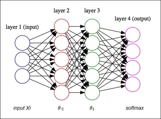
A basic feedforward neural network can easily be depicted by a network diagram, as shown here:
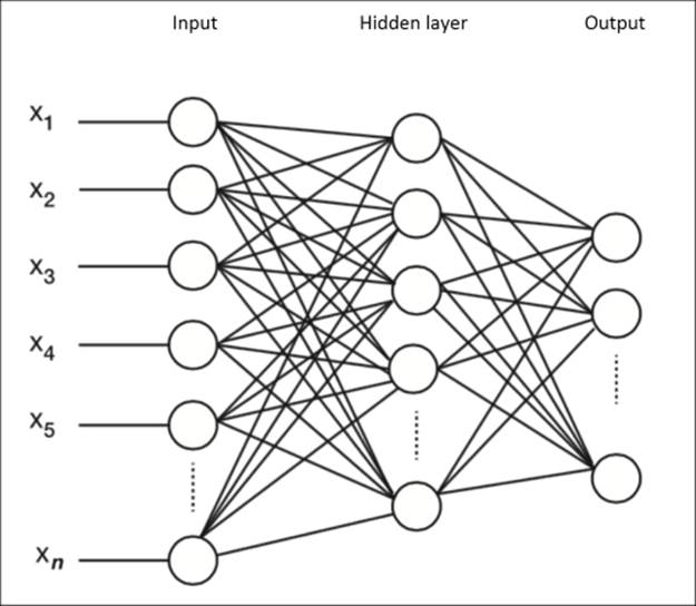
In the network diagram, you can see that this architecture consists of an input layer, hidden layer, and output layer. The input layer contains the feature vectors (where each observation has n features), and the output layer consists of separate units for each class of the output vector in the case of classification and a single numerical vector in the case of regression.
The strength of the connections between the units is expressed through weights later to be passed to an activation function. The goal of an activation function is to transform its input to an output that makes binary decisions more separable.
These activation functions are preferably differentiable so they can be used to learn.
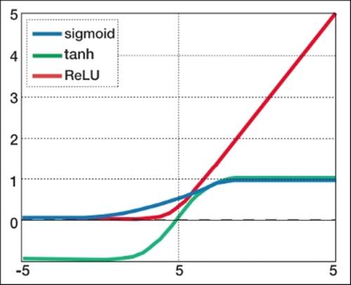
The widely-used activation functions are sigmoid and tanh, and even more recently the rectified linear unit (ReLU) has gained traction. Let's compare the most important activation functions so that we understand their advantages and drawbacks. Note that we mention the output range and active range of the function. The output range is simply the actual output of the function itself. The active range, however, is a little more complicated; it is the range where the gradient has the most variance in the final weight updates. This means that outside of this range, the gradient is near zero and does not add to the parameter updates during learning. This problem of a close-to-zero gradient is also referred to as the vanishing gradient problem and is solved by the ReLU activationfunction, which at this time is the most popular activation for larger neural networks:
It is important to note that features need to be scaled to the active range of the chosen activation function. Most up-to-date packages will have this as a standard preprocessing procedure so you don't need to do this yourself:
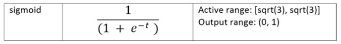
Sigmoid functions are often used for mathematical convenience because their derivatives are very easy to calculate, which we will use to calculate the weight updates in training algorithms:
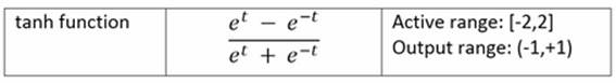
Interestingly the tanh and logistic sigmoid functions are related linearly and tanh can be seen as a rescaled version of the sigmoid function so that its range is between -1 and 1.
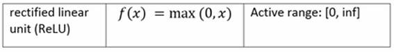
This function is the best choice for deeper architectures. It can be seen as a ramp function whose range lies above 0 to infinity. You can see that it is much easier to calculate than the sigmoid function. The biggest benefit of this function is that it bypasses the vanishing gradient problem. If ReLU is an option during a deep learning project, use it.
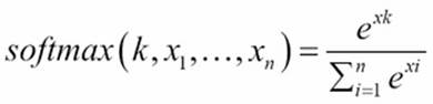
Softmax for classification
So far, we have seen that activation functions transform the values within a certain range after they are multiplied with the weight vectors. We also need to transform the outputs of the last hidden layer before providing balanced classes or probability outputs (log-likelihood values).
This will convert the output of the previous layer to probability values so that a final class prediction can be made. The exponentiation in this case will return a near-zero value whenever the output is significantly less than the maximum of all the values; this way the differences are amplified:
Forward propagation
Now that we understand activation functions and the final outputs of a network, let's see how the input features are fed through the network to provide a final prediction. Computations with huge chunks of units and connections might look like a complex task, but fortunately the feedforward process of a neural network comes down to a sequence of vector computations:
We arrive at a final prediction by performing the following steps:
1. Performing a dot-product on the inputs with the weights between the first and second layer and transforming the result with the activation function.
2. Performing a dot-product on the outputs of the first hidden layer with the weights between the second and third layer. These results are then transformed with the activation function on each unit of the second hidden layer.
3. Finally, we arrive at our prediction by multiplying the vector with the activation function (softmax for classification).
We can treat each layer in the network as a vector and apply simple vector multiplications. More formally, this will look like the following: ![]()
= the weight vector of layer x
b1 and b2 are the bias units
f = the activation function
![]()
![]()
![]()
![]()
Note
Note that this example is based on a single hidden layer network architecture.
Let's perform a simple feedforward pass on a neural network with two hidden layers with basic NumPy. We apply a softmax function to the final output:
import numpy as np
import math
b1=0 #bias unit 1
b2=0 #bias unit 2
def sigmoid(x): # sigmoid function
return 1 /(1+(math.e**-x))
def softmax(x): #softmax function
l_exp = np.exp(x)
sm = l_exp/np.sum(l_exp, axis=0)
return sm
# input dataset with 3 features
X = np.array([ [.35,.21,.33],
[.2,.4,.3],
[.4,.34,.5],
[.18,.21,16] ])
len_X = len(X) # training set size
input_dim = 3 # input layer dimensionality
output_dim = 1 # output layer dimensionality
hidden_units=4
np.random.seed(22)
# create random weight vectors
theta0 = 2*np.random.random((input_dim, hidden_units))
theta1 = 2*np.random.random((hidden_units, output_dim))
# forward propagation pass
d1 = X.dot(theta0)+b1
l1=sigmoid(d1)
l2 = l1.dot(theta1)+b2
#let's apply softmax to the output of the final layer
output=softmax(l2)
Note
Note that the bias unit enables the function to move up and down and will help fit the target values more closely. Each hidden layer consists of one bias unit.
Backpropagation
With our simple feedforward example, we have taken our first steps in training the model. Neural networks are trained quite similarly to gradient descent methods that we have seen with other machine learning algorithms. Namely, we upgrade the parameters of a model in order to find the global minimum of the error function. An important difference with neural networks is that we now have to deal with multiple units across the network that we need to train independently. We do this using the partial derivative of the cost function and calculating how much the error curve drops when we change the particular parameter vector by a certain amount (the learning rate). We start with the layer closest to the output and calculate the gradient with respect to the derivative of our loss function. If there are hidden layers, we move to the second hidden layer and update the weights until the first layer in the feedforward network is reached.
The core idea of backpropagation is quite similar to other machine learning algorithms, with the important complication that we are dealing with multiple layers and units. We have seen that each layer in the network is represented by a weight vector ![]() ij. So, how do we solve this issue? It might seem intimidating that we have to train a large number of weights independently. However, quite conveniently, we can use vectorized operations. Just like we did with the forward pass, we calculate the gradients and update the weights applied to the weight vectors (
ij. So, how do we solve this issue? It might seem intimidating that we have to train a large number of weights independently. However, quite conveniently, we can use vectorized operations. Just like we did with the forward pass, we calculate the gradients and update the weights applied to the weight vectors (![]() ij).
ij).
We can summarize the following steps in the backpropagation algorithm:
1. Feedforward pass: We randomly initialize the weight vectors and multiply the input with the subsequent weight vectors toward a final output.
2. Calculate the error: We calculate the error/loss of the output of the feedforward step.
Randomly initialize the weight vectors.
3. Backpropagation to the last hidden layer (with respect to the output). We calculate the gradient of this error and change weights toward the direction of the gradient. We do this by multiplying the weight vector ![]() j with the gradients performed.
j with the gradients performed.
4. Update the weights till the stopping criterion is reached (minimum error or number of training rounds):
![]()
We have now covered a feedforward pass of an arbitrary two-layer neural network; let's apply backpropagation with SGD in NumPy to the same input that we used in the previous example. Take special note of how we upgrade the weight parameters:
import numpy as np
import math
def sigmoid(x): # sigmoid function
return 1 /(1+(math.e**-x))
def deriv_sigmoid(y): #the derivative of the sigmoid function
return y * (1.0 - y)
alpha=.1 #this is the learning rate
X = np.array([ [.35,.21,.33],
[.2,.4,.3],
[.4,.34,.5],
[.18,.21,16] ])
y = np.array([[0],
[1],
[1],
[0]])
np.random.seed(1)
#We randomly initialize the layers
theta0 = 2*np.random.random((3,4)) - 1
theta1 = 2*np.random.random((4,1)) - 1
for iter in range(205000): #here we specify the amount of training rounds.
# Feedforward the input like we did in the previous exercise
input_layer = X
l1 = sigmoid(np.dot(input_layer,theta0))
l2 = sigmoid(np.dot(l1,theta1))
# Calculate error
l2_error = y - l2
if (iter% 1000) == 0:
print "Neuralnet accuracy:" + str(np.mean(1-(np.abs(l2_error))))
# Calculate the gradients in vectorized form
# Softmax and bias units are left out for instructional simplicity
l2_delta = alpha*(l2_error*deriv_sigmoid(l2))
l1_error = l2_delta.dot(theta1.T)
l1_delta = alpha*(l1_error * deriv_sigmoid(l1))
theta1 += l1.T.dot(l2_delta)
theta0 += input_layer.T.dot(l1_delta)
Now look how the accuracy increases with each pass over the network:
Neuralnet accuracy:0.983345051044
Neuralnet accuracy:0.983404936523
Neuralnet accuracy:0.983464255273
Neuralnet accuracy:0.983523015841
Neuralnet accuracy:0.983581226603
Neuralnet accuracy:0.983638895759
Neuralnet accuracy:0.983696031345
Neuralnet accuracy:0.983752641234
Neuralnet accuracy:0.983808733139
Neuralnet accuracy:0.98386431462
Neuralnet accuracy:0.983919393086
Neuralnet accuracy:0.983973975799
Neuralnet accuracy:0.984028069878
Neuralnet accuracy:0.984081682304
Neuralnet accuracy:0.984134819919
Common problems with backpropagation
One familiar problem with neural networks is that, during optimization with backpropagation, the gradient can get stuck in local minima. This occurs when the error minimization is tricked into seeing a minimum (the point S in the image) where it is really just a local bump to pass the peak S:
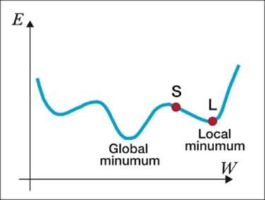
Another common problem is when the gradient descent misses the global minimum, which can sometimes result in surprisingly poor performing models. This problem is referred to as overshooting.
It is possible to solve both these problems by choosing a lower learning rate when the model is overshooting or choose a higher learning rate when getting stuck in local minima. Sometimes this adjustment still doesn't lead to a satisfying and quick convergence. Recently, a range of solutions has been found to mitigate these problems. Learning algorithms with tweaks to the vanilla SGDalgorithms that we just covered have been developed. It is important to understand them so that you can choose the right one for any given task. Let's cover these learning algorithms in more detail.
Backpropagation with mini batch
Batch gradient descent computes the gradient using the whole dataset but backpropagation SGD can also work with so-called mini batches, where a sample of the dataset with size k (batches) is used to update the learning parameter. The amount of error irregularity between each update can be smoothened out with mini batch, which might avoid getting stuck in and overshooting local minima. In most neural network packages, we can change the batch size of the algorithm (we will look at this later). Depending on the amount of training examples, a batch size anywhere between 10 and 300 can be helpful.
Momentum training
Momentum is a method that adds a fraction of the previous weight update to the current one:
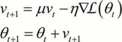
Here, a fraction of the previous weight update is added to the current one. A high momentum parameter can help increase the speed of convergence reaching the global minimum faster. Looking at the formulation, you can see a v parameter. This is the equivalent of the velocity of the gradient updates with a learning rate ![]() . A simple way to understand this is to see that when the gradient keeps pointing in the same direction over multiple instances, the speed of convergence increases with each step toward the minimum. This also removes irregularities between the gradients by a certain margin. Most packages will have this momentum parameter available (as we will see in a later example). When we set this parameter too high, we have to keep in mind that there is a risk of overshooting the global minimum. On the other hand, when we set the momentum parameter too low, the coefficient might get stuck in local minima and can also slow down learning. Ideal settings for the momentum coefficient are normally in the .5 and .99 range.
. A simple way to understand this is to see that when the gradient keeps pointing in the same direction over multiple instances, the speed of convergence increases with each step toward the minimum. This also removes irregularities between the gradients by a certain margin. Most packages will have this momentum parameter available (as we will see in a later example). When we set this parameter too high, we have to keep in mind that there is a risk of overshooting the global minimum. On the other hand, when we set the momentum parameter too low, the coefficient might get stuck in local minima and can also slow down learning. Ideal settings for the momentum coefficient are normally in the .5 and .99 range.
Nesterov momentum
Nesterov momentum is a newer and improved version of classical momentum. In addition to classical momentum training, it will look ahead in the direction of the gradient. In other words, Nesterov momentum takes a simple step going from x to y, and moves a little bit further in that direction so that x to y becomes x to {y (v1 +1)} in the direction given by the previous point. I will spare you the technical details, but remember that it consistently outperforms normal momentum training in terms of convergence. If there is an option for Nesterov momentum, use it.
Adaptive gradient (ADAGRAD)
ADAGRAD provides a feature-specific learning rate that utilizes information from the previous upgrades:
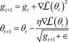
ADAGRAD updates the learning rate for each parameter according to information from previously iterated gradients for that parameter. This is done by dividing each term by the square root of the sum of squares of its previous gradient. This allows the learning rate to decrease over time because the sum of squares will continue to increase with each iteration. A decreasing learning rate has the advantage of decreasing the risk of overshooting the global minimum quite substantially.
Resilient backpropagation (RPROP)
RPROP is an adaptive method that does not look at historical information, but merely looks at the sign of the partial derivative over a training instance and updates the weights accordingly.
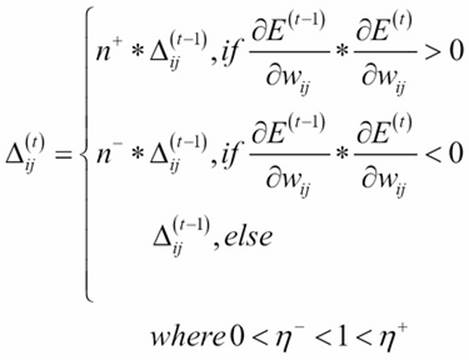
A direct adaptive method for faster backpropagation learning: The RPROP Algorithm. Martin Riedmiller 1993
RPROP is an adaptive method that does not look at historical information, but merely looks at the sign of the partial derivative over a training instance and updates the weights accordingly. Inspecting the preceding image closely, we can see that once the partial derivative of the error changes its sign (> 0 or < 0), the gradient starts moving in the opposite direction, leading toward the global minimum correcting for the overshooting. However, if the sign doesn't change at all, larger steps are taken toward the global minimum. Lots of articles have proven the superiority of RPROP over ADAGRAD but in practice, this is not confirmed consistently. Another important thing to keep in mind is that RPROP does not work properly with mini batches.
RMSProp
RMSProp is an adaptive learning method without shrinking the learning rate:
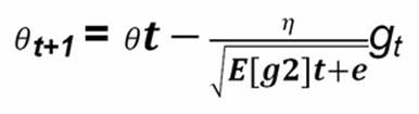
RMSProp is also an adaptive learning method that utilizes ideas from momentum learning and ADAGRAD, with the important addition that it avoids the shrinkage of the learning rate over time. With this technique, the shrinkage is controlled with an exponential decay function over the average of the gradients.
The following is the list of gradient descent optimization algorithms:
|
Applications |
Common problems |
Practical tips |
|
|
Regular SGD |
Widely applicable |
Overshooting, stuck in local minima |
Use with momentum and mini-batch |
|
ADAGRAD |
Smaller datasets <10k |
Slow convergence |
Use a learning rate between .01 and .1. Widely applicable. Works with sparse data |
|
RPROP |
Larger datasets >10k |
Not effective with mini-batches |
Use RMSProp when possible |
|
RMSProp |
Larger datasets >10k |
Not effective with wide and shallow nets |
Particularly useful for wide sparse data |
What and how neural networks learn
Now that we have a basic understanding of backpropagation in all its forms, it is time to address the most difficult task in neural network projects: How do we chose the right architecture? One crucial capability of neural networks is that the weights within an architecture can transform the input into a nonlinear feature space and thereby solve nonlinear classification (decision boundaries) and regression problems. Let's do a simple yet insightful exercise to demonstrate this idea in the neurolab package. We will only useneurolab for a short exercise; for scalable learning problems, we will propose other methods.
First, install the neurolab package with pip.
Install neurolab from the terminal:
> $pip install neurolab
With this example, we will generate a simple nonlinear cosine function with numpy and train a neural network to predict the cosine function from a variable. We will set up several neural network architectures to see how well each architecture is able to predict the cosine target variable:
import neurolab as nl
import numpy as np
from sklearn import preprocessing
import matplotlib.pyplot as plt
plt.style.use('ggplot')
# Create train samples
x = np.linspace(-10,10, 60)
y = np.cos(x) * 0.9
size = len(x)
x_train = x.reshape(size,1)
y_train = y.reshape(size,1)
# Create network with 4 layers and random initialized
# just experiment with the amount of layers
d=[[1,1],[45,1],[45,45,1],[45,45,45,1]]
for i in range(4):
net = nl.net.newff([[-10, 10]],d[i])
train_net=nl.train.train_gd(net, x_train, y_train, epochs=1000, show=100)
outp=net.sim(x_train)
# Plot results (dual plot with error curve and predicted values)
import matplotlib.pyplot
plt.subplot(2, 1, 1)
plt.plot(train_net)
plt.xlabel('Epochs')
plt.ylabel('squared error')
x2 = np.linspace(-10.0,10.0,150)
y2 = net.sim(x2.reshape(x2.size,1)).reshape(x2.size)
y3 = outp.reshape(size)
plt.subplot(2, 1, 2)
plt.suptitle([i ,'hidden layers'])
plt.plot(x2, y2, '-',x , y, '.', x, y3, 'p')
plt.legend(['y predicted', 'y_target'])
plt.show()
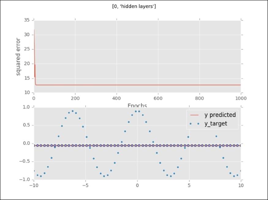
Now look closely at how the error curve behaves and how the predicted values start to approximate the target values as we add more layers to the neural network.
With zero hidden layers, the neural network projects a straight line through the target values. The error curve falls to a minimum quickly with a bad fit:
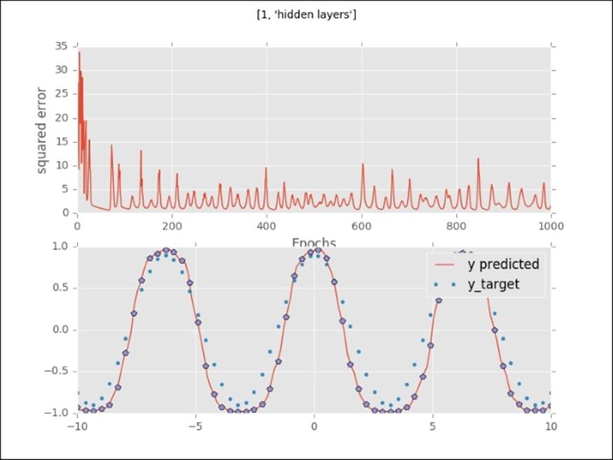
With one hidden layer, the network starts to approximate the target output. Watch how irregular the error curve is:
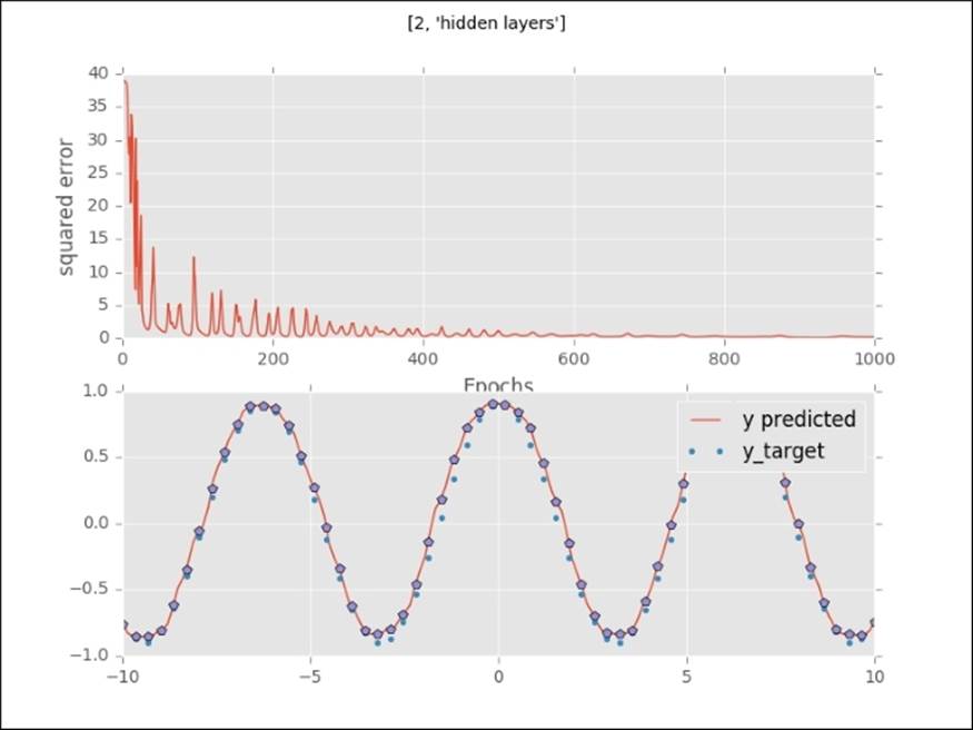
With two hidden layers, the neural network approximates the target value even more closely. The error curve drops faster and behaves less irregularly:
An almost perfect fit with three hidden layers. The error curve drops much faster (around 220 iterations).
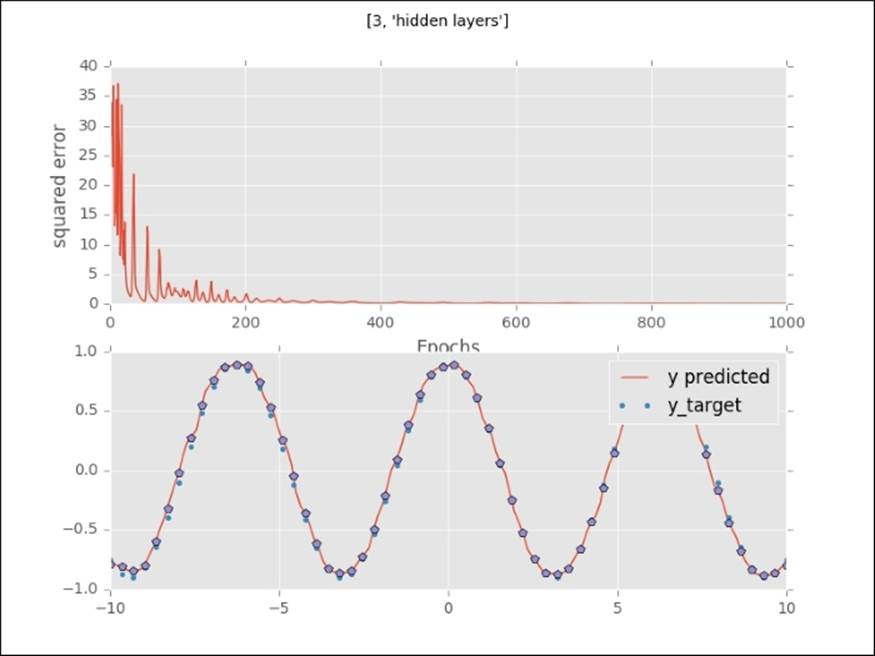
The orange line in the upper plot is a visualization of how the error drops with each epoch (a full pass through the training set). It shows us that we need a certain number of passes through the training set to arrive at a global minimum. If you inspect this error curve more closely, you will see that the error curve behaves differently with each architecture. The lower plot (the dotted line) shows how the predicted values start to approximate the target values. With no hidden layer, the neural network is incapable of detecting nonlinear functions, but once we add hidden layers, the network starts to learn nonlinear functions and increasingly complex functions. In fact, neural networks can learn any possible function. This capability of learning every possible function is called the universal approximation theorem. We can modify this approximation by adding hidden neurons (units and layers) to the neural network. We do need to be cautious, however, that we don't overfit; adding a high amount of layers and units will lead to memorization of the training data instead of fitting a generalizable function. Quite often, too many layers in a network can be detrimental to predictive accuracy.
Choosing the right architecture
As we have seen, the combinatorial space of possible neural network architectures is almost infinite. So how can we know in advance which architecture will be suitable for our project? We need some sort of heuristic or rule of thumb in order to design an architecture for a specific task. In the last section, we used a simple example with only one output and one feature. However, the recent wave of neural network architectures that we refer to as deep learning is very complex and it is crucial to be able to construct the right neural network architectures for any given task. As we have mentioned before, a typical neural network consists of the input layer, one or more hidden layers, and an output layer. Let's look at each layer of the architecture in detail so that we can have a sense of setting up the right architecture for any given task.
The input layer
When we mention the input layer, we are basically talking about the features that will be used as the input of the neural network. The preprocessing steps that are required are highly dependent on the shape and content of the data. If we have features that are measured on different scales, we need to rescale and normalize the data. In cases where we have a high amount of features, a dimension reduction technique such as PCA or SVD will become recommendable.
The following preprocessing techniques can be applied to inputs before learning:
· Normalization, scaling, & outlier detection
· Dimensionality reduction (SVD and factor analysis)
· Pretraining (autoencoders and Boltzmann machines)
We will cover each of these methods in the upcoming examples.
The hidden layer
How do we choose the amount of units in hidden layers? How many hidden layers do we add to the network? We have seen in the the previous example that a neural network without a hidden layer is incapable of learning a nonlinear function (both in curve fitting for regression and in decision boundaries with classification). So if there is a nonlinear pattern or decision boundary to project, we will need hidden layers. When it comes to selecting the amount of units in the hidden layer, we generally want fewer units in the hidden layer than the amount of units in the input layer and more units than the amount of output units:
· Preferably fewer hidden units than the amount of input features
· More units than the amount of output units (classes for classification)
Sometimes, when the target function is very complex in shape, there is an exception. In a case where we add more units than input dimensions, we add an expansion of the feature space. Networks with such layers are commonly referred to as wide networks.
Complex networks can learn more complex functions, but this does not mean that we can simply keep on stacking layers. It is advisory to keep the amount of layers in check because too many layers will cause problems with overfitting, higher CPU load, and even underfitting. Usually between one and four hidden layers will be sufficient.
Tip
Use preferably between one and four layers as a starting point.
The output layer
Each neural network has one output layer and, just like the input layer, is highly dependent on the structure of the data in question. For classification, we will generally use the softmax function. In this case, we should use the same amount of units as the amount of classes we predict.
Neural networks in action
Let's get some hands-on experience with training neural nets for classification. We will use sknn, the Scikit-learn wrapper for lasagne and Pylearn2. You can find out more about the package at https://github.com/aigamedev/scikit-neuralnetwork/.
We will use this tool because of its practical and Pythonic interface. It is a great introduction to more sophisticated frameworks like Keras.
The sknn library can run both on CPU or GPU, whichever you might prefer. Note that if you choose to utilize the GPU, sknn will operate on Theano:
For CPU (most stable) :
# Use the GPU in 32-bit mode, from sknn.platform import gpu32
from sknn.platform import cpu32, threading
# Use the CPU in 64-bit mode.from sknn.platform import cpu64
from sknn.platform import cpu64, threading
GPU:
# Use the GPU in 32-bit mode,
from sknn.platform import gpu32
# Use the CPU in 64-bit mode.
from sknn.platform import cpu64
Parallelization for sknn
We can utilize parallel processing in the following way, but this comes with a warning. It is not the most stable method:
from sknn.platform import cpu64, threading
We can specify Scikit-learn to utilize a specific amount of threads:
from sknn.platform import cpu64, threads2 #any desired amount of threads
When you have specified the appropriate number of threads, you can parallelize your code by implementing n_jobs=nthreads in the cross-validation.
Now that we have covered the most important concepts and prepared our environment, let's implement a neural network.
For this example, we will use the convenient yet rather boring Iris dataset.
After this, we will apply preprocessing in the form of normalization and scaling and start building our model:
import numpy as np
from sklearn.datasets import load_iris
from sknn.mlp import Classifier, Layer
from sklearn import preprocessing
from sklearn.cross_validation import train_test_split
from sklearn import cross_validation
from sklearn import datasets
# import the familiar Iris data-set
iris = datasets.load_iris()
X_train, X_test, y_train, y_test = train_test_split(iris.data,
iris.target, test_size=0.2, random_state=0)
Here we apply preprocessing, normalization, and scaling to our inputs:
X_trainn = preprocessing.normalize(X_train, norm='l2')
X_testn = preprocessing.normalize(X_test, norm='l2')
X_trainn = preprocessing.scale(X_trainn)
X_testn = preprocessing.scale(X_testn)
Let's set up our neural network architecture and parameters. Let's start with a neural network with two layers. In the Layer part, we specify the settings of each layer independently. (We will see this method again in Tensorflow and Keras.) The Iris dataset consists of four features, but because in this particular case a wide neural network works quite well, we will use 13 units in each hidden layer. Note that sknn applies SGD by default:
clf = Classifier(
layers=[
Layer("Rectifier", units=13),
Layer("Rectifier", units=13),
Layer("Softmax")], learning_rate=0.001,
n_iter=200)
model1=clf.fit(X_trainn, y_train)
y_hat=clf.predict(X_testn)
scores = cross_validation.cross_val_score(clf, X_trainn, y_train, cv=5)
print 'train mean accuracy %s' % np.mean(scores)
print 'vanilla sgd test %s' % accuracy_score(y_hat,y_test)
OUTPUT:]
train sgd mean accuracy 0.949909090909
sgd test 0.933333333333
A decent result on the training set, but we might be able to do better.
We talked about how Nesterov momentum can shorten the length toward the global minimum; let's run this algorithm with nesterov to see if we can increase accuracy and improve convergence:
clf = Classifier(
layers=[
Layer("Rectifier", units=13),
Layer("Rectifier", units=13),
Layer("Softmax")], learning_rate=0.001,learning_rule='nesterov',random_state=101,
n_iter=1000)
model1=clf.fit(X_trainn, y_train)
y_hat=clf.predict(X_testn)
scores = cross_validation.cross_val_score(clf, X_trainn, y_train, cv=5)
print 'Nesterov train mean accuracy %s' % np.mean(scores)
print 'Nesterov test %s' % accuracy_score(y_hat,y_test)
OUTPUT]
Nesterov train mean accuracy 0.966575757576
Nesterov test 0.966666666667
Our model is improved with Nesterov momentum in this case.
Neural networks and regularization
Even though we didn't overtrain our model in our last example, it is necessary to think about regularization strategies for neural networks. Three of the most widely-used ways in which we can apply regularization to a neural network are as follows:
· L1 and L2 regularization with weight decay as a parameter for the regularization strength
· Dropout means that deactivating units within the neural network at random can force other units in the network to take over
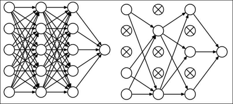
On the left hand, we see an architecture with dropout applied, randomly deactivating units in the network. On the right hand, we see an ordinary neural network (marked with X).
· Averaging or ensembling multiple neural networks (each with different settings)
Let's try dropout for this model and see if works:
clf = Classifier(
layers=[
Layer("Rectifier", units=13),
Layer("Rectifier", units=13),
Layer("Softmax")],
learning_rate=0.01,
n_iter=2000,
learning_rule='nesterov',
regularize='dropout', #here we specify dropout
dropout_rate=.1,#dropout fraction of neural units in entire network
random_state=0)
model1=clf.fit(X_trainn, y_train)
scores = cross_validation.cross_val_score(clf, X_trainn, y_train, cv=5)
print np.mean(scores)
y_hat=clf.predict(X_testn)
print accuracy_score(y_hat,y_test)
OUTPUT]
dropout train score 0.933151515152
dropout test score 0.866666666667
In this case, dropout didn't lead to satisfactory results so we should leave it out altogether. Feel free to experiment with other methods as well. Just change the learning_rule parameter and see what it does to the overall accuracy. The models that you can try aresgd, momentum, nesterov, adagrad, and rmsprop. From this example, you have learned that Nesterov momentum can increase the overall accuracy. In this case, dropout was not the best regularization method and was detrimental to model performance. Considering that this large number of parameters all interact and produce unpredictable results, we really need a tuning method. This is exactly what we are going to do in the next section.
Neural networks and hyperparameter optimization
As the parameter space of neural networks and deep learning models is so wide, optimization is a hard task and computationally very expensive. A wrong neural network architecture can be a recipe for failure. These models can only be accurate if we apply the right parameters and choose the right architecture for our problem. Unfortunately, there are only a few applications that provide tuning methods. We found that the best parameter tuning method at the moment is randomized search, an algorithm that iterates over the parameter space at random sparing computational resources. The sknn library is really the only library that has this option. Let's walk through the parameter tuning methods with the following example based on the wine-quality dataset.
In this example, we first load the wine dataset. Than we apply transformation to the data, from where we tune our model based on chosen parameters. Note that this dataset has 13 features; we specify the units within each layer to be between 4 and 20. We don't use mini-batch in this case; the dataset is simply too small:
import numpy as np
import scipy as sp
import pandas as pd
from sklearn.grid_search import RandomizedSearchCV
from sklearn.grid_search import GridSearchCV, RandomizedSearchCV
from scipy import stats
from sklearn.cross_validation import train_test_split
from sknn.mlp import Layer, Regressor, Classifier as skClassifier
# Load data
df = pd.read_csv('http://archive.ics.uci.edu/ml/machine-learning-databases/wine-quality/winequality-red.csv ' , sep = ';')
X = df.drop('quality' , 1).values # drop target variable
y1 = df['quality'].values # original target variable
y = y1 <= 5 # new target variable: is the rating <= 5?
# Split the data into a test set and a training set
X_train, X_test, y_train, y_test = train_test_split(X, y, test_size=0.2, random_state=42)
print X_train.shape
max_net = skClassifier(layers= [Layer("Rectifier",units=10),
Layer("Rectifier",units=10),
Layer("Rectifier",units=10),
Layer("Softmax")])
params={'learning_rate': sp.stats.uniform(0.001, 0.05,.1),
'hidden0__units': sp.stats.randint(4, 20),
'hidden0__type': ["Rectifier"],
'hidden1__units': sp.stats.randint(4, 20),
'hidden1__type': ["Rectifier"],
'hidden2__units': sp.stats.randint(4, 20),
'hidden2__type': ["Rectifier"],
'batch_size':sp.stats.randint(10,1000),
'learning_rule':["adagrad","rmsprop","sgd"]}
max_net2 = RandomizedSearchCV(max_net,param_distributions=params,n_iter=25,cv=3,scoring='accuracy',verbose=100,n_jobs=1,\
pre_dispatch=None)
model_tuning=max_net2.fit(X_train,y_train)
print "best score %s" % model_tuning.best_score_
print "best parameters %s" % model_tuning.best_params_
OUTPUT:]
[CV] hidden0__units=11, learning_rate=0.100932183167, hidden2__units=4, hidden2__type=Rectifier, batch_size=30, hidden1__units=11, learning_rule=adagrad, hidden1__type=Rectifier, hidden0__type=Rectifier, score=0.655914 - 3.0s
[Parallel(n_jobs=1)]: Done 74 tasks | elapsed: 3.0min
[CV] hidden0__units=11, learning_rate=0.100932183167, hidden2__units=4, hidden2__type=Rectifier, batch_size=30, hidden1__units=11, learning_rule=adagrad, hidden1__type=Rectifier, hidden0__type=Rectifier
[CV] hidden0__units=11, learning_rate=0.100932183167, hidden2__units=4, hidden2__type=Rectifier, batch_size=30, hidden1__units=11, learning_rule=adagrad, hidden1__type=Rectifier, hidden0__type=Rectifier, score=0.750000 - 3.3s
[Parallel(n_jobs=1)]: Done 75 tasks | elapsed: 3.0min
[Parallel(n_jobs=1)]: Done 75 out of 75 | elapsed: 3.0min finished
best score 0.721366278222
best parameters {'hidden0__units': 14, 'learning_rate': 0.03202394348494512, 'hidden2__units': 19, 'hidden2__type': 'Rectifier', 'batch_size': 30, 'hidden1__units': 17, 'learning_rule': 'adagrad', 'hidden1__type': 'Rectifier', 'hidden0__type': 'Rectifier'}
Note
Warning: As the parameter space is searched at random, the results can be inconsistent.
We can see that the best parameters for our model are, most importantly, the first layer with 14 units, the second layer contains 17 units, and the third layer contains 19 units. This is quite a complex architecture that we might never have been able to deduce ourselves, which demonstrates the importance of hyperparameter optimization.
Neural networks and decision boundaries
We have covered in the previous section that, by adding hidden units to a neural network, we can approximate the target function more closely. However, we haven't applied it to a classification problem. To do this, we will generate data with a nonlinear target value and look at how the decision surface changes once we add hidden units to our architecture. Let's see the universal approximation theorem at work! First, let's generate some non-linearly separable data with two features, set up our neural network architectures, and see how our decision boundaries change with each architecture:
%matplotlib inline
from sknn.mlp import Classifier, Layer
from sklearn import preprocessing
import numpy as np
import matplotlib.pyplot as plt
from sklearn import datasets
from itertools import product
X,y= datasets.make_moons(n_samples=500, noise=.2, random_state=222)
from sklearn.datasets import make_blobs
net1 = Classifier(
layers=[
Layer("Softmax")],random_state=222,
learning_rate=0.01,
n_iter=100)
net2 = Classifier(
layers=[
Layer("Rectifier", units=4),
Layer("Softmax")],random_state=12,
learning_rate=0.01,
n_iter=100)
net3 =Classifier(
layers=[
Layer("Rectifier", units=4),
Layer("Rectifier", units=4),
Layer("Softmax")],random_state=22,
learning_rate=0.01,
n_iter=100)
net4 =Classifier(
layers=[
Layer("Rectifier", units=4),
Layer("Rectifier", units=4),
Layer("Rectifier", units=4),
Layer("Rectifier", units=4),
Layer("Rectifier", units=4),
Layer("Rectifier", units=4),
Layer("Softmax")],random_state=62,
learning_rate=0.01,
n_iter=100)
net1.fit(X, y)
net2.fit(X, y)
net3.fit(X, y)
net4.fit(X, y)
# Plotting decision regions
x_min, x_max = X[:, 0].min() - 1, X[:, 0].max() + 1
y_min, y_max = X[:, 1].min() - 1, X[:, 1].max() + 1
xx, yy = np.meshgrid(np.arange(x_min, x_max, 0.1),
np.arange(y_min, y_max, 0.1))
f, arxxx = plt.subplots(2, 2, sharey='row',sharex='col', figsize=(8, 8))
plt.suptitle('Neural Network - Decision Boundary')
for idx, clf, ti in zip(product([0, 1], [0, 1]),
[net1, net2, net3,net4],
['0 hidden layer', '1 hidden layer',
'2 hidden layers','6 hidden layers']):
Z = clf.predict(np.c_[xx.ravel(), yy.ravel()])
Z = Z.reshape(xx.shape)
arxxx[idx[0], idx[1]].contourf(xx, yy, Z, alpha=0.5)
arxxx[idx[0], idx[1]].scatter(X[:, 0], X[:, 1], c=y, alpha=0.5)
arxxx[idx[0], idx[1]].set_title(ti)
plt.show()
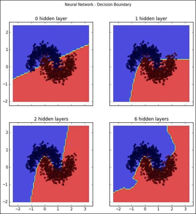
In this screenshot, we can see that, as we add hidden layers to the neural network, we can learn increasingly complex decision boundaries. An interesting side note is that the network with two layers produced the most accurate predictions.
Note
Note that the results might be different between runs.
Deep learning at scale with H2O
In previous sections, we covered neural networks and deep architectures running on a local computer and we found that neural networks are already highly vectorized but still computationally expensive. There is not much that we can do if we want to make the algorithm more scalable on a desktop computer other than utilizing Theano and GPU computing. So if we want to scale deep learning algorithms more drastically, we will need to find a tool that can run algorithms out-of-core instead of on a local CPU/GPU. H2O is, at this moment, the only open source out-of-core platform that can run deep learning algorithms quickly. It is also cross-platform; besides Python, there are APIs for R, Scala, and Java.
H2O is compiled on a Java-based platform developed for a wide range of data science-related tasks such as datahandling and machine learning. H2O runs on distributed and parallel CPUs in-memory so that data will be stored in the H2O cluster. The H2O platform—as of yet—has applications for General Linear Models (GLM), Random Forests, Gradient Boosting Machines (GBM), K Means, Naive Bayes, Principal Components Analysis, Principal Components Regression, and, of course our main focus for this chapter, Deep Learning.
Great, now we are ready to perform our first H2O out-of-core analysis.
Let's start the H2O instance and load a file in H2O's distributed memory system:
import sys
sys.prefix = "/usr/local"
import h2o
h2o.init(start_h2o=True)
Type this to get interesting information about the specifications of your cluster.
Look at the memory that is allowed and the number of cores.
h2o.cluster_info()
This will look more or less like the following (slight differences might occur between trials and systems):
OUTPUT:]
Java Version: java version "1.8.0_60"
Java(TM) SE Runtime Environment (build 1.8.0_60-b27)
Java HotSpot(TM) 64-Bit Server VM (build 25.60-b23, mixed mode)
Starting H2O JVM and connecting: .................. Connection successful!
------------------------------ ---------------------------------------
H2O cluster uptime: 2 seconds 346 milliseconds
H2O cluster version: 3.8.2.3
H2O cluster name: H2O_started_from_python**********nzb520
H2O cluster total nodes: 1
H2O cluster total free memory: 3.56 GB
H2O cluster total cores: 8
H2O cluster allowed cores: 8
H2O cluster healthy: True
H2O Connection ip: 1**.***.***.***
H2O Connection port: 54321
H2O Connection proxy:
Python Version: 2.7.10
------------------------------ ---------------------------------------
------------------------------ ---------------------------------------
H2O cluster uptime: 2 seconds 484 milliseconds
H2O cluster version: 3.8.2.3
H2O cluster name: H2O_started_from_python_quandbee_nzb520
H2O cluster total nodes: 1
H2O cluster total free memory: 3.56 GB
H2O cluster total cores: 8
H2O cluster allowed cores: 8
H2O cluster healthy: True
H2O Connection ip: 1**.***.***.***
H2O Connection port: 54321
H2O Connection proxy:
Python Version: 2.7.10
------------------------------ ---------------------------------------
Sucessfully closed the H2O Session.
Successfully stopped H2O JVM started by the h2o python module.
Large scale deep learning with H2O
In H2O deep learning, the dataset that we will use to train is the famous MNIST dataset. It consists of pixel intensities of 28 x 28 images of handwritten digits. The training set has 70,000 training items with 784 features together with a label for each record containing the target label digits.
Now that we are more comfortable with managing data in H2O, let's perform a deep learning example.
In H2O, we don't have to transform or normalize the input data; it is standardized internally and automatically. Each feature is transformed into the N(0,1) space.
Let's import the famous handwritten digits image dataset MNIST from the Amazon server to the H2O cluster:
import h2o
h2o.init(start_h2o=True)
train_url ="https://h2o-public-test-data.s3.amazonaws.com/bigdata/laptop/mnist/train.csv.gz"
test_url="https://h2o-public-test-data.s3.amazonaws.com/bigdata/laptop/mnist/test.csv.gz"
train=h2o.import_file(train_url)
test=h2o.import_file(test_url)
train.describe()
test.describe()
y='C785'
x=train.names[0:784]
train[y]=train[y].asfactor()
test[y]=test[y].asfactor()
from h2o.estimators.deeplearning import H2ODeepLearningEstimator
model_cv=H2ODeepLearningEstimator(distribution='multinomial'
,activation='RectifierWithDropout',hidden=[32,32,32],
input_dropout_ratio=.2,
sparse=True,
l1=.0005,
epochs=5)
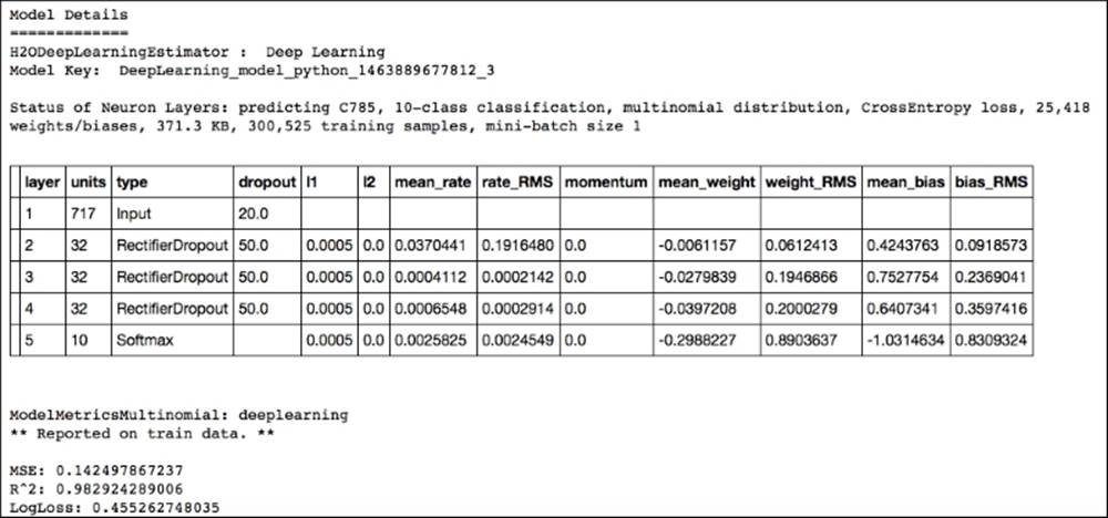
The output of this print model will provide a lot of detailed information. The first table that you will see is the following one. This provides all the specifics about the architecture of the neural network. You can see that we have used a neural network with an input dimension of 717 with three hidden layers (consisting of 32 units each) with softmax activation applied to the output layer and ReLU between the hidden layers:
model_cv.train(x=x,y=y,training_frame=train,nfolds=3)
print model_cv
OUTPUT]
If you want a short overview of model performance, this is a very practical method.
In the following table, the most interesting metrics are the training classification error and validation classification error over each fold. You can easily compare these in case you want to validate your model:
print model_cv.scoring_history()
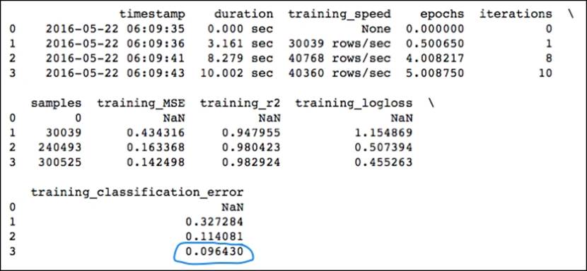
Our training classification error of .096430 and accuracy in the .907 range on the MNIST dataset is pretty good; it's almost as good as Yann LeCun's convolutional neural network submission.
H2O provides a convenient method to acquire validation metrics as well. We can do this by passing the validation dataframe to the cross-validation function:
model_cv.train(x=x,y=y,training_frame=train,validation_frame=test,nfolds=3)
print model_cv
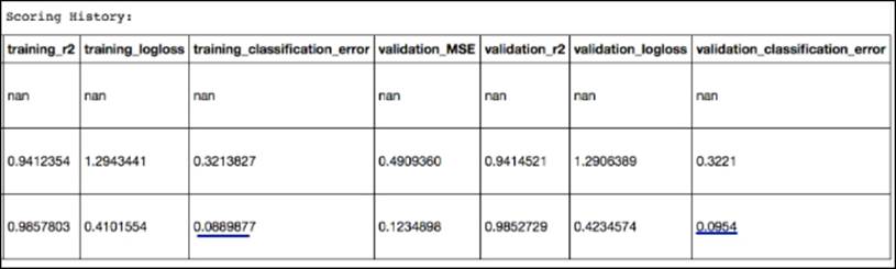
In this case, we can easily compare training_classification_error (.089) with our validation_classification_error (.0954).
Maybe we can improve our score; let's use a hyperparameter optimization model.
Gridsearch on H2O
Considering that our previous model performed quite well, we will focus our tuning efforts on the architecture of our network. H2O's gridsearch function is quite similar to Scikit-learn's randomized search; namely, instead of searching the full parameter space, it iterates over a random list of parameters. First, we will set up a parameter list that we will pass to the gridsearch function. H2O will provide us with an output of each model and the corresponding score in the parameters' search:
hidden_opt = [[18,18],[32,32],[32,32,32],[100,100,100]]
# l1_opt = [s/1e6 for s in range(1,1001)]
# hyper_parameters = {"hidden":hidden_opt, "l1":l1_opt}
hyper_parameters = {"hidden":hidden_opt}
#important: here we specify the search parameters
#be careful with these, training time can explode (see max_models)
search_c = {"strategy":"RandomDiscrete",
"max_models":10, "max_runtime_secs":100,
"seed":222}
from h2o.grid.grid_search import H2OGridSearch
model_grid = H2OGridSearch(H2ODeepLearningEstimator, hyper_params=hyper_parameters)
#We have added a validation set to the gridsearch method in order to have a better #estimate of the model performance.
model_grid.train(x=x, y=y, distribution="multinomial", epochs=1000, training_frame=train, validation_frame=test,
score_interval=2, stopping_rounds=3, stopping_tolerance=0.05,search_criteria=search_c)
print model_grid
# Grid Search Results for H2ODeepLearningEstimator:
OUTPUT]
deeplearning Grid Build Progress: [##################################################] 100%
hidden \
0 [100, 100, 100]
1 [32, 32, 32]
2 [32, 32]
3 [18, 18]
model_ids logloss
0 Grid_DeepLearning_py_1_model_python_1464790287811_3_model_3 0.148162 ←------
1 Grid_DeepLearning_py_1_model_python_1464790287811_3_model_2 0.173675
2 Grid_DeepLearning_py_1_model_python_1464790287811_3_model_1 0.212246
3 Grid_DeepLearning_py_1_model_python_1464790287811_3_model_0 0.227706
We can see that our best architecture would be one with three layers with 100 units each. We can also clearly see that gridsearch increases training time substantially even on a powerful computing cluster like the one that H2O operates on. So, even on H2O, we should use gridsearch with caution and be conservative with the parameters that are parsed in the model.
Now let's shutdown the H2O instance before we proceed:
h2o.shutdown(prompt=False)
Deep learning and unsupervised pretraining
In this section, we will introduce the most important concept in deep learning: how to improve learning by unsupervised pretraining. With unsupervised pretraining, we use neural networks to find latent features and factors in the data to later pass to a neural network. This method has the powerful capability of training networks to learn tasks that other machine learning methods can't, without handcrafting features. We will get into the specifics and introduce a new powerful library.
Deep learning with theanets
Scikit-learn's neural network application is especially interesting for parameter tuning purposes. Unfortunately, its capabilities for unsupervised neural network applications are limited. For the next subject, where we dive into more sophisticated deep learning methods, we need another library. In this chapter, we will focus on theanets. We love theanets because of its ease of use and stability; it's a very smooth and well-maintained package developed by Lief Johnson at the University of Texas. Setting up a neural network architecture works quite similarly to sklearn; namely, we instantiate a learning objective (classification or regression), specify the layers, and train it. For more information, you can visit http://theanets.readthedocs.org/en/stable/.
All you have to do is install theanets with pip:
$ pip install theanets
As theanets is built on top of Theano, you also need to have the Theano properly installed. Let's run a basic neural network model to see how theanets works. The resemblance with Scikit-learn will be obvious. Note that we use momentum for this example, and softmax is used by default in theanets so we don't have to specify it:
import climate # This package provides the reporting of iterations
from sklearn.metrics import confusion_matrix
import numpy as np
from sklearn import datasets
from sklearn.cross_validation import train_test_split
from sklearn.metrics import mean_squared_error
import theanets
import theano
import numpy as np
import matplotlib.pyplot as plt
import climate
from sklearn.cross_validation import train_test_split
import theanets
from sklearn.metrics import confusion_matrix
from sklearn import preprocessing
from sklearn.metrics import accuracy_score
from sklearn import datasets
climate.enable_default_logging()
digits = datasets.load_digits()
digits = datasets.load_digits()
X = np.asarray(digits.data, 'float32')
Y = digits.target
Y=np.array(Y, dtype=np.int32)
#X = (X - np.min(X, 0)) / (np.max(X, 0) + 0.0001) # 0-1 scaling
X_train, X_test, y_train, y_test = train_test_split(X, Y,
test_size=0.2,
random_state=0)
# Build a classifier model with 64 inputs, 1 hidden layer with 100 units and 10 outputs.
net = theanets.Classifier([64,100,10])
# Train the model using Resilient backpropagation and momentum.
net.train([X_train,y_train], algo='sgd', learning_rate=.001, momentum=0.9,patience=0,
validate_every=N,
min_improvement=0.8)
# Show confusion matrices on the training/validation splits.
print(confusion_matrix(y_test, net.predict(X_test)))
print (accuracy_score(y_test, net.predict(X_test)))
OUTPUT ]
[[27 0 0 0 0 0 0 0 0 0]
[ 0 32 0 0 0 1 0 0 0 2]
[ 0 1 34 0 0 0 0 1 0 0]
[ 0 0 0 29 0 0 0 0 0 0]
[ 0 0 0 0 29 0 0 1 0 0]
[ 0 0 0 0 0 38 0 0 0 2]
[ 0 1 0 0 0 0 43 0 0 0]
[ 0 0 0 0 1 0 0 38 0 0]
[ 0 2 1 0 0 0 0 0 36 0]
[ 0 0 0 0 0 1 0 0 0 40]]
0.961111111111
Autoencoders and unsupervised learning
Up until now, we discussed neural networks with multiple layers and a wide variety of parameters to optimize. The current generation of neural networks that we often refer to as deep learning is capable of more; it is capable of learning new features automatically so that very little feature engineering and domain expertise is required. These features are created by unsupervised methods on unlabeled data later to be fed into a subsequent layer in a neural network. This method is referred to as (unsupervised) pretraining. This approach has been proven to be highly successful in image recognition, language learning, and even vanilla machine learning projects. The most important and dominant technique in recent years is called denoising autoencoders and algorithms based on Boltzmann techniques. Boltzmann machines, which were the building blocks for Deep Belief Networks (DBN), have lately fallen out of favor in the deep learning community because they turned out to be hard to train and optimize. For this reason, we will focus only on autoencoders. Let's cover this important topic in small manageable steps.
Autoencoders
We try to find a function (F) that has an output as its input with the least possible error F(x)≈ 'x. This function is commonly referred to as the identity function, which we try to optimize so that x is as close as possible to 'x. The difference between x and 'x is referred to as reconstruction error.
Let's look at a simple single-layer architecture to get an intuition of what's going on. We will see that these architectures are very flexible and need careful tuning:
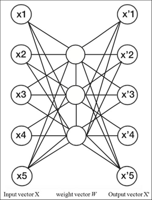
Single-layer autoencoder architecture
It is important to understand that when we have fewer units in the hidden layer than the input space, we force the weights to compress the input data.
In this case, we have a dataset containing five features. In the middle is a hidden layer containing three units (Wij). These units have the same property as the weight vector that we have seen in neural networks; namely, they are made up of weights that can be trained with backpropagation. With the output of the hidden layer, we get the feature representations as output by the same feedforward vector operations as we have seen with neural networks.
The process of calculating the vector 'x is quite similar to what we have seen with forward propagation by calculating the dot products of the weight vectors of each layer:
W=the weights
![]()
![]()
The reconstruction error can be measured with the squared error or in cross-entropy form, which we have seen in so many other methods. In this case, ŷ represents the reconstructed output and y the true input:
![]()
An important notion is that, with only one hidden layer, the dimensions in the data captured by the autoencoder model approximate the results of Principal Component Analysis (PCA). However, an autoencoder behaves much differently if there is non-linearityinvolved. The autoencoder will detect different latent factors that PCA will never be able to detect. Now that we know more about the architecture of the autoencoder and how we can calculate the error from its identity approximation, let's look at these sparsity parameters with which we compress the input.
You might ask: why do we even need this scarcity parameter? Can't we just run the algorithm to find the identity function and move on?
Unfortunately, it is not quite that simple. There are cases where the identity function projects the input almost perfectly but still fails to extract the latent dimensions of the input features. In that case, the function simply memorizes the input data instead of extracting meaningful features. We can do two things. First, we deliberately add noise to the signal (denoising autoencoders) and second, we introduce a sparsity parameter, forcing the deactivation of weakly-activated units. Let's first look at how sparsity works.
We discussed the activation threshold of a biological neuron; we can think of a neuron as being active if its potential is close to 1 or being inactive if its output value is close to 0. We can constraint the neurons to be inactive most of the time by increasing the activation threshold. We do this by decreasing the average activation probability of each neuron/unit. Looking at the following formula, we can see how we can minimize the activation threshold:
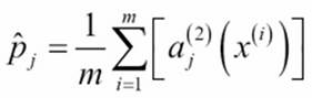
![]() j: The average activation threshold of each neuron in the hidden layer.
j: The average activation threshold of each neuron in the hidden layer.
ρ: The desired activation threshold of the network, which we specify upfront. In most cases, this value is set at .05.
a: The weight vector of the hidden layers.
Here, we see an opportunity for optimization by penalizing a training round on the error rate between ![]() j and ρ.
j and ρ.
In this chapter, we will not worry too much about the technical details of this optimization objective. In most packages, we can use a very simple instruction to do this (as we will see in the next example). The most important thing to understand is that with autoencoders, we have two main learning objectives: minimizing the error between the input vector x and output vector 'x by optimizing the identity function, and minimizing the difference between the desired activation threshold and average activation of each neuron in the network.
The second way in which we can force the autoencoder to detect latent features is by introducing noise in the model; this is where the name denoising autoencoders comes from. The idea is that by corrupting the input, we force the autoencoder to learn a more robust representation of the data. In the upcoming example, we will simply introduce Gaussian noise to the auto-encoder model.
Really deep learning with stacked denoising autoencoders – pretraining for classification
With this exercise, you will set yourself apart from the many people who talk about deep learning and the few who actually do it! Now we will apply an autoencoder to the mini version of the famous MNIST dataset, which can conveniently be loaded from within Scikit-learn. The dataset consists of pixel intensities of 28 x 28 images of handwritten digits. The training set has 1,797 training items with 64 features with a label for each record containing the target label digits from 0 to 9. So we have 64 features with a target variable consisting of 10 classes (digits from 0-9) to predict.
First, we train the stacked denoising autoencoder model with a sparsity of .9 and inspect the reconstruction error. We will use the results from deep learning research papers as a guideline for the settings. You can read this paper for more information (http://arxiv.org/pdf/1312.5663.pdf). However, we have some limitations because of the enormous computational load for these types of models. So, for this autoencoder, we use five layers with ReLU activation and compress the data from 64 features to 45 features:
model = theanets.Autoencoder([64,(45,'relu'),(45,'relu'),(45,'relu'),(45,'relu'),(45,'relu'),64])
dAE_model=model.train([X_train],algo='rmsprop',input_noise=0.1,hidden_l1=.001,sparsity=0.9,num_updates=1000)
X_dAE=model.encode(X_train)
X_dAE=np.asarray(X_dAE, 'float32')
:OUTPUT:
I 2016-04-20 05:13:37 downhill.base:232 RMSProp 2639 loss=0.660185 err=0.645118
I 2016-04-20 05:13:37 downhill.base:232 RMSProp 2640 loss=0.660031 err=0.644968
I 2016-04-20 05:13:37 downhill.base:232 validation 264 loss=0.660188 err=0.645123
I 2016-04-20 05:13:37 downhill.base:414 patience elapsed!
I 2016-04-20 05:13:37 theanets.graph:447 building computation graph
I 2016-04-20 05:13:37 theanets.losses:67 using loss: 1.0 * MeanSquaredError (output out:out)
I 2016-04-20 05:13:37 theanets.graph:551 compiling feed_forward function
Now we have the output from our autoencoder that we created from a new set of compressed features. Let's look closer at this new dataset:
X_dAE.shape
Output: (1437, 45)
Here, we can actually see that we have compressed the data from 64 to 45 features. The new dataset is less sparse (meaning fewer zeroes) and numerically more continuous. Now that we have our pretrained data from the autoencoder, we can apply a deep neural network to it for supervised learning:
#By default, hidden layers use the relu transfer function so we don't need to specify #them. Relu is the best option for auto-encoders.
# Theanets classifier also uses softmax by default so we don't need to specify them.
net = theanets.Classifier(layers=(45,45,45,10))
autoe=net.train([X_dAE, y_train], algo='rmsprop',learning_rate=.0001,batch_size=110,min_improvement=.0001,momentum=.9,
nesterov=True,num_updates=1000)
## Enjoy the rare pleasure of 100% accuracy on the training set.
OUTPUT:
I 2016-04-19 10:33:07 downhill.base:232 RMSProp 14074 loss=0.000000 err=0.000000 acc=1.000000
I 2016-04-19 10:33:07 downhill.base:232 RMSProp 14075 loss=0.000000 err=0.000000 acc=1.000000
I 2016-04-19 10:33:07 downhill.base:232 RMSProp 14076 loss=0.000000 err=0.000000 acc=1.000000
Before we predict this neural network on the test set, it is important that we apply the autoencoder model that we have trained to the test set:
dAE_model=model.train([X_test],algo='rmsprop',input_noise=0.1,hidden_l1=.001,sparsity=0.9,num_updates=100)
X_dAE2=model.encode(X_test)
X_dAE2=np.asarray(X_dAE2, 'float32')
Now let's check the performance on the test set:
final=net.predict(X_dAE2)
from sklearn.metrics import accuracy_score
print accuracy_score(final,y_test)
OUTPUT: 0.972222222222
We can see that the final accuracy of the model with auto-encoded features (.9722) outperforms the model without it (.9611).
Summary
In this chapter, we looked at the most important concepts behind deep learning together with scalable solutions.
We took away some of the black-boxiness by learning how to construct the right architecture for any given task and worked through the mechanics of forward propagation and backpropagation. Updating the weights of a neural network is a hard task, regular stochastic gradient descent can result in getting stuck in global minima or overshooting. More sophisticated algorithms like momentum, ADAGRAD, RPROP and RMSProp can provide solutions. Even though neural networks are harder to train than other machine learning methods, they have the power of transforming feature representations and can learn any given function (universal approximation theorem). We also dived into large scale deep learning with H2O, and even utilized the very hot topic of parameter optimization for deep learning.
Unsupervised pre-training with auto-encoders can increase accuracy of any given deep network and we walked through a practical example within the theanets framework to get there.
In this chapter, we primarily worked with packages built on top of the Theano framework. In the next chapter, we will cover deep learning techniques with packages built on top of the new open source framework Tensorflow.
All materials on the site are licensed Creative Commons Attribution-Sharealike 3.0 Unported CC BY-SA 3.0 & GNU Free Documentation License (GFDL)
If you are the copyright holder of any material contained on our site and intend to remove it, please contact our site administrator for approval.
© 2016-2026 All site design rights belong to S.Y.A.