Large Scale Machine Learning with Python (2016)

Chapter 5. Deep Learning with TensorFlow

In this chapter, we will focus on TensorFlow and cover the following topics:

· Basic TensorFlow operations

· Machine learning from scratch with TensorFlow—regression, SGD classifier, and neural network

· Deep learning with SkFlow

· Incremental deep learning with large files

· Convolutional Neural Networks with Keras

The TensorFlow framework was introduced at the time of writing this book and already has proven to be a great addition to the machine learning landscape.

TensorFlow was started by the Google Brain Team consisting of most of the researchers that worked on important developments in deep learning in the recent decade (Geoffrey Hinton, Samy Bengio, and others). It is basically a next-generation development of an earlier generation of frameworks called DistBelief, a platform for distributed deep neural networks. Contrary to TensorFlow, DistBelief is not open source. Interesting examples of successful DistBelief projects are the reversed image search engine, Google deep dream, and speech recognition in Google apps. DistBelief enabled Google developers to utilize thousands of cores (both CPU and GPU) for distributed training.

TensorFlow is an improvement over DistBelief in that it is now completely open source and its programming language is less abstract. TensorFlow claims to be more flexible and has a wider range of applications. At the time of writing (late 2015), the TensorFlow framework is in its infancy and interesting lightweight packages built on top of TensorFlow have already emerged, as we will see later in this chapter.

Similarly to Theano, TensorFlow operates with symbolic computations on tensors; this means that most of its computations are based on vector-and matrix multiplications.

Regular programming languages define variables that contain values or characters to which operations can be applied to.

In symbolic programming languages such as Theano or TensorFlow, operations are structured around graphs instead of variables. This has computational advantages because they can be distributed and parallelized across computational units (GPU and CPU):

Deep Learning with TensorFlow

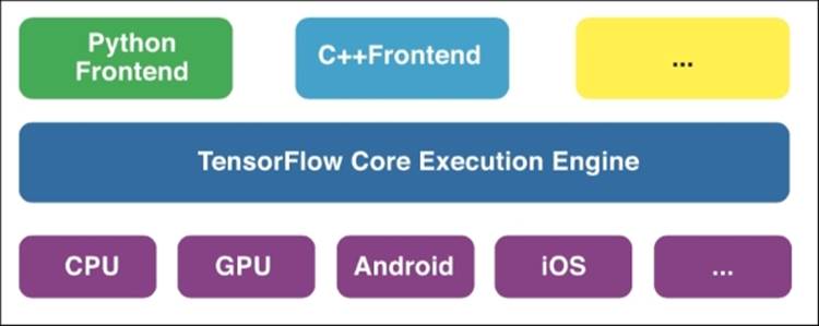
TensorFlow's architecture as introduced in November 2015

Tensorflow has the following features and applications:

· TensorFlow can be parallelized (horizontally) with multiple GPUs

· A development framework is also available for mobile deployment

· TensorBoard is a dashboard for visualizations (at a premature stage)

· It's a frontend for several programming languages (Python Go, Java, Lua, JavaScript, R, C++, and soon Julia)

· It provides integration for large scale solutions such as Spark and Google Cloud Platform (https://cloud.google.com/ml/)

The idea that tensor operations in a graph-like structure provide new ways of parallelized computations (so Google claims) can become quite clear with the following image:

Deep Learning with TensorFlow

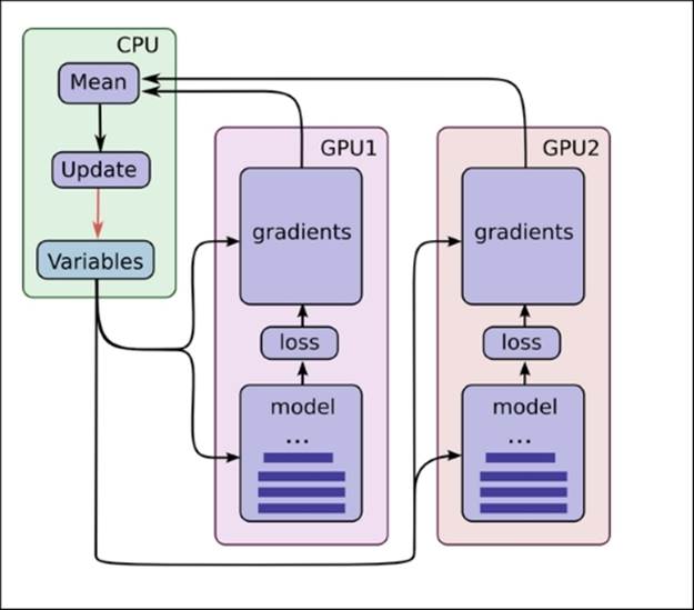
A distributed processing architecture with TensorFlow

We can see from this image that each model can be assigned to separate GPUs. After which the average of the predictions is calculated from each model. Among other methods, this approach has been the central idea to train very large distributed neural networks on GPU clusters.

TensorFlow installation

The version of TensorFlow that we will use in this chapter is 0.8 so make sure that you install this version. As TensorFlow is in heavy development, small changes are due. We can install TensorFlow quite easily with pip install, independent of which operating system you use:

pip install tensorflow

If you already have previous versions installed, you can upgrade according to your operating system:

# Ubuntu/Linux 64-bit, CPU only:

$ sudo pip install --upgrade https://storage.googleapis.com/tensorflow/linux/cpu/tensorflow-0.8.1-cp27-none-linux_x86_64.whl

# Ubuntu/Linux 64-bit, GPU enabled:

$ sudo pip install --upgrade https://storage.googleapis.com/tensorflow/linux/gpu/tensorflow-0.8.1-cp27-none-linux_x86_64.whl

# Mac OS X, CPU only:

$ sudo easy_install --upgrade six

$ sudo pip install --upgrade https://storage.googleapis.com/tensorflow/mac/tensorflow-0.8.1-cp27-none-any.whl

Now that TensorFlow is installed, you can test it in the terminal:

$python

import tensorflow as tf

hello = tf.constant('Hello, TensorFlow!')

sess = tf.Session()

print(sess.run(hello))

Output Hello, TensorFlow!

TensorFlow operations

Let's walk through some simple examples to get a feel for how it works.

An important distinction is that with TensorFlow, we first need to initialize the variables before we can apply operations to them. TensorFlow operates on a C++ backend to perform computations so, in order to connect to this backend, we need to instantiate a session first:

x = tf.constant([22,21,32], name='x')

d=tf.constant([12,23,43],name='x')

y = tf.Variable(x * d, name='y')

print(y)

Instead of providing the output vector of x*d, you will see something like this:

OUTPUT ]

<tensorflow.python.ops.variables.Variable object at 0x114a95710>

To actually produce the provided results of a computation from the C++ backend, we instantiate the session in the following way:

x = tf.constant([22,21,32], name='x')

d=tf.constant([12,23,43],name='d')

y = tf.Variable(x * d, name='y')

model = tf.initialize_all_variables()

with tf.Session() as session:

session.run(model)

print(session.run(y))

Output [ 264 483 1376]

Up until now, we have used variables directly, but to be more flexible with tensor operations, it can be convenient if we can assign data to a prespecified container. This way, we can perform operations on the computation graph without loading the data in-memory beforehand. In TensorFlow terminology, we then feed data into the graph through what are called placeholders. This is exactly where the resemblance with the Theano language becomes clear (see the Appendix, Introduction to GPUs and Theano).

These TensorFlow placeholders are simply containers of objects with certain prespecified settings and classes. So in order to perform operations on an object, we first create a placeholder for that object, together with its corresponding class (an integer in this case):

a = tf.placeholder(tf.int8)

b = tf.placeholder(tf.int8)

sess = tf.Session()

sess.run(a+b, feed_dict={a: 111, b: 222})

Output 77

Matrix multiplications will work like this:

matrix1 = tf.constant([[1, 2,32], [3, 4,2],[3,2,11]])

matrix2 = tf.constant([[21,3,12], [3, 56,2],[35,21,61]])

product = tf.matmul(matrix1, matrix2)

with tf.Session() as sess:

result = sess.run(product)

print result

OUTPUT

[[1147 787 1968]

[ 145 275 166]

[ 454 352 711]]

It is interesting to note that the output of the object result is a NumPy ndarray object that we can apply operations to outside of TensorFlow.

GPU computing

If we want to perform TensorFlow operations on a GPU, we only need to specify a device. Be warned; this only works with a properly installed, CUDA-compatible, NVIDIA GPU unit:

with tf.device('/gpu:0'):

product = tf.matmul(matrix1, matrix2)

with tf.Session() as sess:

result = sess.run(product)

print result

If we want to utilize multiple GPUs, we need to assign a GPU device to a specific task:

matrix3 = tf.constant([[13, 21,53], [4, 3,6],[3,1,61]])

matrix4 = tf.constant([[13,23,32], [23, 16,2],[35,51,31]])

with tf.device('/gpu:0'):

product = tf.matmul(matrix1, matrix2)

with tf.Session() as sess:

result = sess.run(product)

print result

with tf.device('/gpu:1'):

product = tf.matmul(matrix3, matrix4)

with tf.Session() as sess:

result = sess.run(product)

print result

Linear regression with SGD

Now that we have covered the basics, we can start writing our first machine learning algorithm from scratch within the TensorFlow framework. Later, we will use more practical lightweight applications in higher abstractions on top of TensorFlow.

We will perform a very simple linear regression with stochastic gradient descent in order to get a sense of how training and evaluation works in TensorFlow. First, we will create some variables to work with in order to parse them in placeholders to contain those variables. We then feed x and y to a cost function and train the model with gradient descent:

import tensorflow as tf

import numpy as np

X = tf.placeholder("float") # create symbolic variables

Y = tf.placeholder("float")

X_train = np.asarray([1,2.2,3.3,4.1,5.2])

Y_train = np.asarray([2,3,3.3,4.1,3.9,1.6])

def model(X, w):

return tf.mul(X, w)

w = tf.Variable(0.0, name="weights")

y_model = model(X, w) # our predicted values

cost = (tf.pow(Y-y_model, 2)) # squared error cost

train_op = tf.train.GradientDescentOptimizer(0.01).minimize(cost) #sgd optimization

sess = tf.Session()

init = tf.initialize_all_variables()

sess.run(init)

for trials in range(50): #

for (x, y) in zip(X_train, Y_train):

sess.run(train_op, feed_dict={X: x, Y: y})

print(sess.run(w))

OUTPUT ]

0.844732

To summarize, we perform linear regression with SGD in the following way: first, we initialize the regression weights (coefficients), then in the second step, we set up the cost function to later train and optimize the function with gradient descent. In the end, we need to write a for loop in order to specify the amount of training rounds we want and calculate the final predictions. The same basic structure will become apparent in neural networks.

A neural network from scratch in TensorFlow

Now let's perform a neural network in the TensorFlow language and dissect the process.

We will also use the Iris dataset and some Scikit-learn applications to preprocess in this case:

import tensorflow as tf

import numpy as np

from sklearn import cross_validation

from sklearn.cross_validation import train_test_split

from sklearn.preprocessing import OneHotEncoder

from sklearn.utils import shuffle

from sklearn import preprocessing

import os

import pandas as pd

from datetime import datetime as dt

import logging

iris = datasets.load_iris()

X = np.asarray(iris.data, 'float32')

Y = iris.target

from sklearn import preprocessing

X= preprocessing.scale(X)

min_max_scaler = preprocessing.MinMaxScaler()

X = min_max_scaler.fit_transform(X)

lb = preprocessing.LabelBinarizer()

Y=lb.fit_transform(iris.target)

This is an important step. Neural networks in TensorFlow cannot work with target labels within a singular vector. Target labels need to be transformed into binarized features (some will know this as dummy variables) so that the neural network will work with a one versus all output:

X_train, x_test, y_train, y_test = train_test_split(X,Y,test_size=0.3,random_state=22)

def init_weights(shape):

return tf.Variable(tf.random_normal(shape, stddev=0.01))

Here, we can see the feedforward pass:

def model(X, w_h, w_o):

h = tf.nn.sigmoid(tf.matmul(X, w_h))

return tf.matmul(h, w_o)

X = tf.placeholder("float", [None, 4])

Y = tf.placeholder("float", [None, 3])

Here, we set up our layer architecture with one hidden layer:

w_h = init_weights([4, 4])

w_o = init_weights([4, 3])

py_x = model(X, w_h, w_o)

cost = tf.reduce_mean(tf.nn.softmax_cross_entropy_with_logits(py_x, Y)) # compute costs

train_op = tf.train.GradientDescentOptimizer(learning_rate=0.01).minimize(cost) # construct an optimizer

predict_op = tf.argmax(py_x, 1)

sess = tf.Session()

init = tf.initialize_all_variables()

sess.run(init)

for i in range(500):

for start, end in zip(range(0, len(X_train),1 ), range(1, len(X_train),1)):

sess.run(train_op, feed_dict={X: X_train[start:end], Y: y_train[start:end]})

if i % 100 == 0:

print i, np.mean(np.argmax(y_test, axis=1) ==

sess.run(predict_op, feed_dict={X: x_test, Y: y_test}))

OUTPUT:]

0 0.288888888889

100 0.666666666667

200 0.933333333333

300 0.977777777778

400 0.977777777778

The accuracy of this neural network is around .977% but can yield slightly different results across runs. It is more or less the benchmark for a neural network with a single hidden layer and vanilla SGD.

Like we saw in the previous examples, it is quite intuitive to implement an optimization method and set up the tensors. It is a lot more intuitive than when we do the same in NumPy. (See Chapter 4, Neural Networks and Deep Learning.) The downside at this moment is that evaluation and prediction requires a sometimes tedious for loop, whereas packages such as Scikit-learn can provide these methods with a simple line of script. Luckily, there are higher-level packages developed on top of TensorFlow that make training and evaluation a lot easier. One of those packages is SkFlow; as the name implies, it is a wrapper based on a scripting style that works just like Scikit-learn.

Machine learning on TensorFlow with SkFlow

Now that we have seen the basic operations of TensorFlow, let's dive into the higher-level applications built on top of TensorFlow to make machine learning a little more practical. SkFlow is the first application that we will cover. In SkFlow, we don't have to specify types and placeholders. We can load and manage data in the same way that we would do with Scikit-learn and NumPy. Let's install the package with pip.

The safest way is to install the package from GitHub directly:

$ pip install git+git://github.com/tensorflow/skflow.git

SkFlow has three main classes of learning algorithms: linear classifiers, linear regression, and neural networks. A linear classifier is basically a simple SGD (multi) classifier, and neural networks is where SkFlow excels. It provides relatively easy-to-use wrappers for very deep neural networks, recurrent networks, and Convolutional Neural Networks. Unfortunately, other algorithms such as Random Forest, gradient boosting, SVM, and Naïve Bayes are not yet implemented. However, there were discussions on GitHub about implementing a Random Forest algorithm in SkFlow that will probably be named tf_forest, which is an exciting development.

Let's apply our first multiclass classification algorithm in SkFlow. For this example, we will use the wine dataset—a dataset originally from the UCI machine learning repository. It consists of 13 features of continuous chemical metrics such as Magnesium, Alcohol, Malic acid, and so on. It's a light dataset with only 178 instances and a target feature with three classes. The target variable consists of three different cultivars. Wines are classified according to their respective cultivar (type of grapes used for the wine) using the chemical analysis of the thirteen chemical metrics. You can see that we load the data from a URL in the same way that we would do it when we work in a Scikit-learn environment:

import numpy as np

from sklearn.metrics import accuracy_score

import skflow

import urllib2

url = 'https://www.csie.ntu.edu.tw/~cjlin/libsvmtools/datasets/multiclass/wine.scale'

set1 = urllib2.Request(url)

wine = urllib2.urlopen(set1)

from sklearn.datasets import load_svmlight_file

X_train, y_train = load_svmlight_file(wine)

X_train=X_train.toarray()

from sklearn.cross_validation import train_test_split

X_train, X_test, y_train, y_test = train_test_split(X_train,

y_train, test_size=0.30, random_state=4)

classifier = skflow.TensorFlowLinearClassifier(n_classes=4,learning_rate=0.01, optimizer='SGD',continue_training=True, steps=1000)

classifier.fit(X_train, y_train)

score = accuracy_score(y_train, classifier.predict(X_train))

d=classifier.predict(X_test)

print("Accuracy: %f" % score)

c=accuracy_score(d,y_test)

print('validation/test accuracy: %f' % c)

OUTPUT:

Step #1, avg. loss: 1.58672

Step #101, epoch #25, avg. loss: 1.45840

Step #201, epoch #50, avg. loss: 1.09080

Step #301, epoch #75, avg. loss: 0.84564

Step #401, epoch #100, avg. loss: 0.68503

Step #501, epoch #125, avg. loss: 0.57680

Step #601, epoch #150, avg. loss: 0.50120

Step #701, epoch #175, avg. loss: 0.44486

Step #801, epoch #200, avg. loss: 0.40151

Step #901, epoch #225, avg. loss: 0.36760

Accuracy: 0.967742

validation/test accuracy: 0.981481

By now, this method will be quite familiar; it is basically the same way a classifier in Scikit-learn would work. However, there are two important things to notice. With SkFlow, we can use NumPy and TensorFlow objects interchangeably so that we don't have to merge and convert objects in and out of tensor frames. This makes working with TensorFlow through a higher-level method like SkFlow much more flexible. The second thing to notice is that we applied the toarray method to the main data object. This is because the dataset is quite sparse (lots of zero entries), and TensorFlow is not able to process sparse data well.

Neural networks is where TensorFlow excels and in SkFlow, it is quite easy to train a neural network with multiple layers. Let's perform a neural network on the diabetes dataset. This dataset contains diabetes metrics (binary target) diagnostic features of pregnant females of over 21 years of age and of Pima heritage. The Pima Indians of Arizona have the highest reported prevalence of diabetes of any population in the world and therefore this ethnic group has been a voluntary subject of diabetes research. The dataset consists of the following features:

· Number of times pregnant

· Plasma glucose concentration at two hours in an oral glucose tolerance test

· Diastolic blood pressure (mm Hg)

· Triceps skin fold thickness (mm)

· 2-hour serum insulin (mu U/ml)

· Body mass index (weight in kg/(height in m)^2)

· Diabetes pedigree function

· Age (years)

· Class variable (0 or 1)

In this example, we first load and scale the data:

import tensorflow

import tensorflow as tf

import numpy as np

import urllib

import skflow

from sklearn.preprocessing import Normalizer

from sklearn import datasets, metrics, cross_validation

from sklearn.cross_validation import train_test_split

# Pima Indians Diabetes dataset (UCI Machine Learning Repository)

url = "http://archive.ics.uci.edu/ml/machine-learning-databases/pima-indians-diabetes/pima-indians-diabetes.data"

# download the file

raw_data = urllib.urlopen(url)

dataset = np.loadtxt(raw_data, delimiter=",")

print(dataset.shape)

X = dataset[:,0:7]

y = dataset[:,8]

X_train, X_test, y_train, y_test = train_test_split(X, y,

test_size=0.2,

random_state=0)

from sklearn import preprocessing

X= preprocessing.scale(X)

min_max_scaler = preprocessing.MinMaxScaler()

X = min_max_scaler.fit_transform(X)

This step is very interesting; for neural networks to converge better, we can use more flexible decay rates. While training multilayer neural networks, it is usually helpful to decrease the learning rate over time. Generally speaking, when we have a too high learning rate, we might overshoot the optimum. On the other hand, when the learning rate is too low, we will waste computational resources and get stuck in local minima. Exponential decay is a method to dampen the learning rate over time so that it becomes more sensitive when it starts to approach a minimum. There are three common ways of implementing the learning rate decay; namely, step decay, 1/t decay, and exponential decay:

Exponential decay: a=a₀e^−kt

In this case, a is the learning rate, k is the hyperparameter, and t is the iteration.

In this example, we will use exponential decay because it seemed to have worked very well for this dataset. This is how we implement an exponential decay function (with TensorFlow's built-in tf.train.exponential_decay function):

def exp_decay(global_step):

return tf.train.exponential_decay(

learning_rate=0.01, global_step=global_step,

decay_steps=steps, decay_rate=0.01)

We can now pass the decay function in the TensorFlow neural network model. For this neural network, we will provide a two-layer network, with the first layer consisting of five units and the second layer of four units. By default, SkFlow implements the ReLU activation function as we prefer it over the other ones (tanh, sigmoid, and so on) and so we stick with it.

Following this example, we can also implement optimization algorithms other than stochastic gradient descent. Let's implement an adaptive algorithm called Adam based on an article by Diederik Kingma and Jimmy Ba (http://arxiv.org/abs/1412.6980).

Adam, developed in the University of Amsterdam, stands for adaptive moment estimation. In the previous chapter, we saw how ADAGRAD works—by lowering the gradients over time as they move toward the (hopefully) global minimum. Adam also uses adaptive methods, but in combination with the idea of momentum training where previous gradient updates are taken into account:

steps = 5000

classifier = skflow.TensorFlowDNNClassifier(

hidden_units=[5,4],

n_classes=2,

batch_size=300,

steps=steps,

optimizer='Adam',#SGD #RMSProp

learning_rate=exp_decay #here is the decay function

)

classifier.fit(X_train,y_train)

score1a = metrics.accuracy_score(y_train, classifier.predict(X_train))

print("Accuracy: %f" % score1a)

score1b = metrics.accuracy_score(y_test, classifier.predict(X_test))

print("Validation Accuracy: %f" % score1b)

OUTPUT

(768, 9)

Step #1, avg. loss: 12.83679

Step #501, epoch #167, avg. loss: 0.69306

Step #1001, epoch #333, avg. loss: 0.56356

Step #1501, epoch #500, avg. loss: 0.54453

Step #2001, epoch #667, avg. loss: 0.54554

Step #2501, epoch #833, avg. loss: 0.53300

Step #3001, epoch #1000, avg. loss: 0.53266

Step #3501, epoch #1167, avg. loss: 0.52815

Step #4001, epoch #1333, avg. loss: 0.52639

Step #4501, epoch #1500, avg. loss: 0.52721

Accuracy: 0.754072

Validation Accuracy: 0.740260

The accuracy is not so convincing; we might improve the accuracy by applying Principal Component Analysis (PCA) to the input. In this article by Stavros J Perantonis and Vassilis Virvilis from 1999 (http://rexa.info/paper/dc4f2babc5ca4534b435280aec32f5816ddb53b0), it has been proposed that this diabetes dataset benefits well from a PCA dimension reduction before passing in the neural network. We will use the Scikit-learn pipeline method for this dataset:

from sklearn.decomposition import PCA

from sklearn import linear_model, decomposition, datasets

from sklearn.pipeline import Pipeline

from sklearn.metrics import accuracy_score

pca = PCA(n_components=4,whiten=True)

lr = pca.fit(X)

classifier = skflow.TensorFlowDNNClassifier(

hidden_units=[5,4],

n_classes=2,

batch_size=300,

steps=steps,

optimizer='Adam',#SGD #RMSProp

learning_rate=exp_decay

)

pipe = Pipeline(steps=[('pca', pca), ('NNET', classifier)])

X_train, X_test, Y_train, Y_test = train_test_split(X, y,

test_size=0.2,

random_state=0)

pipe.fit(X_train, Y_train)

score2 = metrics.accuracy_score(Y_test, pipe.predict(X_test))

print("Accuracy Validation, with pca: %f" % score2)

OUTPUT:

Step #1, avg. loss: 1.07512

Step #501, epoch #167, avg. loss: 0.54236

Step #1001, epoch #333, avg. loss: 0.50186

Step #1501, epoch #500, avg. loss: 0.49243

Step #2001, epoch #667, avg. loss: 0.48541

Step #2501, epoch #833, avg. loss: 0.46982

Step #3001, epoch #1000, avg. loss: 0.47928

Step #3501, epoch #1167, avg. loss: 0.47598

Step #4001, epoch #1333, avg. loss: 0.47464

Step #4501, epoch #1500, avg. loss: 0.47712

Accuracy Validation, with pca: 0.805195

We have been able to improve the performance of the neural network quite a bit with that simple PCA preprocessing step. We went from seven features to a reduction of four dimensions, thus four features. PCA generally smoothens the signal by zero-centering the features, reducing the feature space using only the vectors containing the highest eigenvalue. Whitening makes sure that the features are transformed into zero-correlated ones. This results in a smoother signal and smaller feature set enabling the neural network to converge faster. See the Chapter 7, Unsupervised Learning at Scale for a more detailed explanation of PCA.

Deep learning with large files – incremental learning

Until now, we have dealt with some TensorFlow operations and machine learning techniques on SkFlow on relatively small datasets. However, this book is about large scale and scalable machine learning; what has the TensorFlow framework to offer us in that regard?

Until recently, parallel computation was in its infancy and not stable enough to be covered in this book. Multi-GPU computing is not accessible to readers without CUDA-compatible NVIDIA cards. Large scale cloud services (https://cloud.google.com/products/machine-learning/) or Amazon EC2 come with a considerable fee. This leaves only one way we can scale our project—by incremental learning.

Generally speaking, any file size exceeding about 25% of the available RAM of a computer will cause memory overload problems. So if you have a 2 GB computer and want to apply machine learning solutions to a 500 MB file, it is time to start thinking about ways to bypass memory consumption.

In order to prevent memory overload, we advise an out-of-core learning method that breaks the data down into smaller chunks to incrementally train and update models. The partial fit methods in Scikit-learn that we covered in Chapter 2, Scalable Learning in Scikit-learn, are examples of this.

SkFlow also provides a great incremental learning method for all its machine learning models just like the partial fit method in Scikit-learn. In this section, we are going to use a deep learning classifier incrementally because we think it is the most exciting one.

In this section, we will use two strategies for our scalable and out-of-core deep learning project; namely, incremental learning and random subsampling.

First, we generate some data, then we build a subsample function where we can draw random subsamples from that dataset and incrementally train a deep learning model on these subsets:

import numpy as np

import pandas as pd

import skflow

from sklearn.datasets import make_classification

import random

from sklearn.cross_validation import train_test_split

import gc

import tensorflow as tf

from sklearn.metrics import accuracy_score

First, we are going to generate some example data and write it to disk:

X, y = make_classification(n_samples=5000000,n_features=10, n_classes=4,n_informative=6,random_state=222,n_clusters_per_class=1)

X_train, X_test, y_train, y_test = train_test_split(X,y, test_size=0.2, random_state=22)

Big_trainm=pd.DataFrame(X_train,y_train)

Big_testm = pd.DataFrame(X_test,y_test)

Big_trainm.to_csv('lsml-Bigtrainm', sep=',')

Big_testm.to_csv('lsml-Bigtestm', sep=',')

Let's free up memory by deleting all the objects that we created.

With gc.collect we force Python's garbage collector to empty memory:

del(X,y,X_train,y_train,X_test)

gc.collect

Here, we create a function that draws random subsamples from disk. Note that we use a sample fraction of ⅓. We could use smaller fractions but we also need to adjust two important things if we do so. First, we need to match the batch size of the deep learning model so that the batch size never exceeds the sample size. Second, we need to adjust our amount of epochs in our for loop in such a way that we make sure that the largest portion of the training data is used to train the model:

import pandas as pd

import random

def sample_file():

global skip_idx

global train_data

global X_train

global y_train

big_train='lsml-Bigtrainm'

Count the number of rows in the entire set:

num_lines = sum(1 for i in open(big_train))

We use one-third fraction of the training set:

size = int(num_lines / 3)

Skip indexes and keep indices:

skip_idx = random.sample(range(1, num_lines), num_lines - size)

train_data = pd.read_csv(big_train, skiprows=skip_idx)

X_train=train_data.drop(train_data.columns[[0]], axis=1)

y_train = train_data.ix[:,0]

We saw weight decay in a previous section; we will use it again here:

def exp_decay(global_step):

return tf.train.exponential_decay(

learning_rate=0.01, global_step=global_step,

decay_steps=steps, decay_rate=0.01)

Here, we set up our neural network DNN classifier with three hidden layers with 5, 4, and 4 units respectively. Note that we set the batch size to 300, which means that we use 300 training cases in each epoch. This also helps prevent memory from overloading:

steps = 5000

clf = skflow.TensorFlowDNNClassifier(

hidden_units=[5,4,4],

n_classes=4,

batch_size=300,

steps=steps,

optimizer='Adam',

learning_rate=exp_decay

)

Here, we set our amount of subsamples to three (epochs=3). This means that we incrementally train our deep learning model on three consecutive subsamples:

epochs=3

for i in range(epochs):

sample_file()

clf.partial_fit(X_train,y_train)

test_data = pd.read_csv('lsml-Bigtestm',sep=',')

X_test=test_data.drop(test_data.columns[[0]], axis=1)

y_test = test_data.ix[:,0]

score = accuracy_score(y_test, clf.predict(X_test))

print score

OUTPUT

Step #501, avg. loss: 0.55220

Step #1001, avg. loss: 0.31165

Step #1501, avg. loss: 0.27033

Step #2001, avg. loss: 0.25250

Step #2501, avg. loss: 0.24156

Step #3001, avg. loss: 0.23438

Step #3501, avg. loss: 0.23113

Step #4001, avg. loss: 0.23335

Step #4501, epoch #1, avg. loss: 0.23303

Step #1, avg. loss: 2.57968

Step #501, avg. loss: 0.57755

Step #1001, avg. loss: 0.33215

Step #1501, avg. loss: 0.27509

Step #2001, avg. loss: 0.26172

Step #2501, avg. loss: 0.24883

Step #3001, avg. loss: 0.24343

Step #3501, avg. loss: 0.24265

Step #4001, avg. loss: 0.23686

Step #4501, epoch #1, avg. loss: 0.23681

0.929022

We managed to get an accuracy of .929 on the test set within a very manageable training time and without overloading our memory, considerably faster than if we would have trained the same model on the entire dataset at once.

Keras and TensorFlow installation

Previously, we have seen practical examples of the SkFlow wrapper for TensorFlow applications. For a more sophisticated approach to neural networks and deep learning where we have more control over parameters, we propose Keras (http://keras.io/). This package was originally developed within the Theano framework, but recently is also adapted to TensorFlow. This way, we can use Keras as a higher abstract package on top of TensorFlow. Keep in mind though that Keras is slightly less straightforward than SkFlow in its methods. Keras can run on both GPU and CPU, which makes this package really flexible when porting it to different environments.

Let's first install Keras and make sure that it utilizes the TensorFlow backend.

Installation works simply using pip in the command line:

$pip install Keras

Keras is originally built on top of Theano, so we need to specify Keras to utilize TensorFlow instead. In order to do this, we first need to run Keras once on its default platform, Theano.

First, we need to run some Keras code to make sure that all the library items are properly installed. Let's train a basic neural network and get introduced to some key concepts.

Out of convenience, we will make use of generated data with Scikit-learn consisting of four features and a target variable consisting of three classes. These dimensions are very important because we need them to specify the architecture of the neural network:

import numpy as np

import keras

from sklearn.datasets import make_classification

from sklearn.cross_validation import train_test_split

from sklearn.preprocessing import OneHotEncoder

from keras.utils import np_utils, generic_utils

from keras.models import Sequential

from keras.layers import Dense, Dropout, Activation

from keras.optimizers import SGD

nb_classes=3

X, y = make_classification(n_samples=1000, n_features=4, n_classes=nb_classes,n_informative=3, n_redundant=0, random_state=101)

Now that we have specified the variables, it is important to convert the target variable to a one-hot encoding array (just like we did in TensorFlow). Otherwise, Keras won't be able to compute the one versus all target outputs. For Keras, we want to use np_utilsinstead of sklearn's one-hot encoder. This is how we will use it:

y=np_utils.to_categorical(y,nb_classes)

print y

Our array of y will look like this:

OUTPUT]

array([[ 1., 0., 0.],

[ 0., 0., 1.],

…,

Now let's split the data into test and train:

x_train, x_test, y_train, y_test = train_test_split(X, y,test_size=0.30, random_state=222)

This is where we start to give form to the neural network architecture that we have in mind. Let's start a two-hidden layer neural network with relu activation and three units in each hidden layer. Our first layer has four inputs because we have four features in this case. After that, we add the hidden layers with three units, hence (model.add(dense(3)).

Like we have seen before, we will use a softmax function to pass the network to the output layer:

model = Sequential()

model.add(Dense(4, input_shape=(4,)))

model.add(Activation('relu'))

model.add(Dense(3))

model.add(Activation('relu'))

model.add(Dense(3))

model.add(Activation('softmax'))

First, we specify our SGD function, where we implement the most important parameters that are familiar to us by now, namely:

· lr: The learning rate.

· decay: The decay function to decay the learning rate. Do not confuse this with weight decay, which is a regularization parameter.

· momentum: We use this to prevent from getting stuck in local minima.

· nesterov: This is a Boolean that specifies whether we want to use nesterov momentum and is only applicable if we have specified an integer for the momentum parameter. (Refer to Chapter 4, Neural Networks and Deep Learning, for a more detailed explanation.)

· optimizer: Here, we will specify our optimization algorithm of choice (consisting of SGD, RMSProp, ADAGRAD, Adadelta, and Adam).

Let us see the following code snippet:

#We use this for reproducibility

seed = 22

np.random.seed(seed)

model = Sequential()

model.add(Dense(4, input_shape=(4,)))

model.add(Activation('relu'))

model.add(Dense(3))

model.add(Activation('relu'))

model.add(Dense(3))

model.add(Activation('softmax'))

sgd = SGD(lr=0.01, decay=1e-6, momentum=0.9, nesterov=True)

model.compile(loss='categorical_crossentropy', optimizer=sgd)

model.fit(x_train, y_train, verbose=1, batch_size=100, nb_epoch=50,show_accuracy=True,validation_data=(x_test, y_test))

time.sleep(0.1)

In this case, we have used batch_size of 100, which means that we have used minibatch gradient descent with 100 training examples in each epoch. In this model, we have used 50 training epochs. This will give you the following output:

OUTPUT:

acc: 0.8129 - val_loss: 0.5391 - val_acc: 0.8000

Train on 700 samples, validate on 300 samples

In the last model where we used SGD with nesterov, we couldn't improve our score no matter how many epochs we used for its training.

In order to increase accuracy. it is advisable to try out other optimization algorithms. We have already used the Adam optimization method successfully before, so let's use it again here and see if we can increase the accuracy. As adaptive learning rates such as Adam, lower the learning rate over time, it requires more epochs to arrive at an optimum solution. Therefore, in this example, we will set the amount of epochs to 200:

adam=keras.optimizers.Adam(lr=0.01)

model.compile(loss='categorical_crossentropy', optimizer=adam)

model.fit(x_train, y_train, verbose=1, batch_size=100, nb_epoch=200,show_accuracy=True,validation_data=(x_test, y_test))

time.sleep(0.1)

OUTPUT:

Epoch 200/200

700/700 [==============================] - 0s - loss: 0.3755 - acc: 0.8657 - val_loss: 0.4725 - val_acc: 0.8200

We now have managed to achieve a convincing improvement from 0.8 to 0.82 with the Adam optimization algorithm.

For now, we have covered the most important elements of neural networks in Keras. Let's now proceed setting up Keras so that it will utilize the TensorFlow framework. By default, Keras will use the Theano backend. In order to instruct Keras to work on TensorFlow, we need to first locate the Keras folder in the packages folder:

import os

print keras.__file__

Your path might look different:

Output: /Library/Python/2.7/site-packages/keras/__init__.pyc

Now that we have located the package folder of Keras, we need to look for the ~/.keras/keras.json file.

There is a piece of script in this file that looks like this:

{"epsilon": 1e-07, "floatx": "float32", "backend": "theano"}

You simply need to change "backend":"theano" to "backend":"tensorflow", resulting in the following:

{"epsilon": 1e-07, "floatx": "float32", "backend": "tensorflow"}

If, for some reason, the .json file is not present in the Keras folder, that is, /Library/Python/2.7/site-packages/keras/, you can just copy paste this to a text editor:

{"epsilon": 1e-07, "floatx": "float32", "backend": "tensorflow"}

Save it as a .json file and put it in the keras folder.

To test if the TensorFlow environment is properly utilized from within TensorFlow, we can type the following:

from keras import backend as K

input = K.placeholder(shape=(4, 4, 5))

# also works:

input = K.placeholder(shape=(None, 2, 5))

# also works:

input = K.placeholder(ndim=2)

OUTPUT:

Using Theano backend.

Some users might get no output at all, which is fine. Your TensorFlow backend should be ready to use.

Convolutional Neural Networks in TensorFlow through Keras

Between this and the previous chapter, we have come quite a long way covering the most important topics in deep learning. We now understand how to construct architectures by stacking multiple layers in a neural network and how to discern and utilize backpropagation methods. We also covered the concept of unsupervised pretraining with stacked and denoising autoencoders. The next and really exciting step in deep learning is the rapidly evolving field of Convolutional Neural Networks (CNN), a method of building multilayered, locally connected networks. CNNs, commonly referred to as ConvNets, are so rapidly evolving at the time of writing this book that we literally had to rewrite and update this chapter within a month's timeframe. In this chapter, we will cover the most fundamental and important concepts behind CNNs so that we will be able to run some basic examples without becoming overwhelmed by the sometimes enormous complexity. However, we won't be able to do justice fully to the enormous theoretical and computational background so this paragraph provides a practical starting point.

The best way to understand CNNs conceptually is to go back in history, start with a little bit of cognitive neuroscience, and look at Huber and Wiesel's research on the visual cortex of cats. Huber and Wiesel recorded neuro-activations of the visual cortex in cats while measuring neural activity by inserting microelectrodes in the visual cortex of the brain. (Poor cats!) They did this while the cats were watching primitive images of shapes projected on a screen. Interestingly, they found that certain neurons responded only to contours of specific orientation or shape. This led to the theory that the visual cortex is composed of local and orientation-specific neurons. This means that specific neurons respond only to images of specific orientation and shape (triangles, circles, or squares). Considering that cats and other mammals can perceive complex and evolving shapes into a coherent whole, we can assume that perception is an aggregate of all these locally and hierarchically organized neurons. By that time, the first multilayer perceptrons were already fully developed so it didn't take too long before this idea of locality and specific sensitivity in neurons was modeled in perceptron architectures. From a computational neuroscience perspective, this idea was developed into maps of local receptive regions in the brain with the addition of selectively connected layers. This was adopted by the already ongoing field of neural networks and artificial intelligence. The first reported scientist who applied this notion of local specific computationally to a multilayer perceptron was Fukushima with his so-called neocognitron (1982).

Yann LeCun developed the idea of the neocognitron into his version called LeNet. It added the gradient descent backpropagation algorithm. This LeNet architecture is still the foundation for many more evolved CNN architectures introduced recently. A basic CNN like LeNet learns to detect edges from raw pixels in the first layer, then use these edges to detect simple shapes in the second layer, and later in the process uses these shapes to detect higher-level features, such as objects in an environment in higher layers. The layer further down the neural sequence is then a final classifier that uses these higher-level features. We can see the feedforward pass in a CNN like this: we move from a matrix input to pixels, we detect edges from pixels, then shapes from edges, and detect increasingly distinctive and more abstract and complex features from shapes.

Note

Each convolution or layer in the network is receptive for a specific feature (such as shape, angle, or color).

Deeper layers will combine these features into a more complex aggregate. This way, it can process complete images without burdening the network with the full input space of the image at step.

Up until now, we have only worked with fully connected neural networks where each layer is connected to each neighboring layer. These networks have proven to be quite effective, but have the downside of dramatically increasing the number of parameters that we have to train. On a side note, we might imagine that when we train a small image (28 x 28) in size, we can get away with a fully connected network. However, training a fully connected network on larger images that span across the entire image would be tremendously computationally expansive.

Note

To summarize, we can state that CNNs have the following benefits over fully connected neural networks:

· They reduce the parameter space and thus prevent overtraining and computational load

· CNNs are invariant to object orientation (think of face recognition classifying faces with different locations)

· CNNs capable of learning and generalizing complex multidimensional features

· CNNs can be usefull in speech recogntion, image classification, and lately complex recommendation engines

CNNs utilize so-called receptive fields to connect the input to a feature map. The best way to understand CNNs is to dive deeper into the architecture, and of course get hands-on experience. So let's run through the types of layers that make up CNNs. The architecture of a CNN consists of three types of layers; namely, convolutional layer, pooling layer, and a fully-connected layer, where each layer accepts an input 3D volume (h, w, d) and transforms it into a 3D output through a differentiable function.

The convolution layer

We can understand the concept of convolution by imagining a spotlight of a certain size sliding over the input (pixel-values and RGB color dimensions), conveniently after which we compute a dot product between the filtered values (also referred to as patches) and the true input. This does two important things: first, it compresses the input, and more importantly, second, the network learns filters that only activate when they see some specific type of feature spatial position in the input.

Look at the following image to see how this works:

The convolution layer

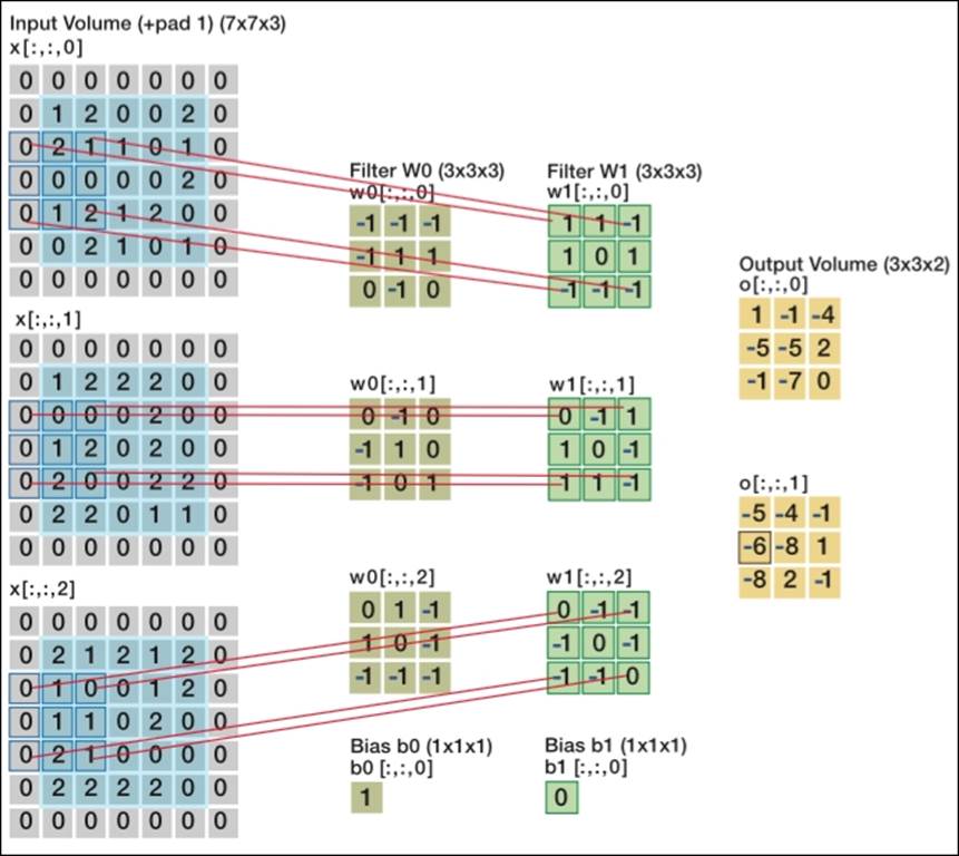
Two convolutional layers processing image input [7x7x3] input volume: an image of width 7, height 7, and with three color channels R,G,B

We can see from this image that we have two levels of filters (W0 and W1) and three dimensions (in the form of arrays) of inputs, all resulting in the dot product of the sliding spotlight/window over the input matrix. We refer to the size of this spotlight as stride, whichmeans that the larger the stride, the smaller the output.

As you can see, when we apply a 3 x 3 filter, the full scope of the filter is processed at the center of the matrix, but once we move close to or past the edges, we start to lose out on the edges of the input. In this case, we apply what is called zero-padding. All elements that fall outside of the input dimensions are set to zero in this case. Zero-padding became more or less a default setting for most CNN applications recently.

The pooling layer

The next type of layer that is often placed in between the filter layers is called a pooling layer or subsampling layer. What this does is it performs a downsampling operation along the spatial dimensions (width, height), which in turn helps with overfitting and reducingcomputational load. There are several ways to perform this downsampling, but recently Max Pooling turned out to be the most effective method.

Max-pooling is a simple method that compresses features by taking the maximum value of a patch of the neighboring feature. The following image will clarify this idea; each color box within the matrix represents a subsample of stride size 2:

The pooling layer

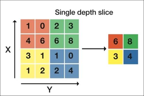
A max-pooling layer with a stride of 2

The pooling layers are used mainly for the following reasons:

· Reduce the amount of parameters and thus computational load

· Regularization

Interestingly, the latest research findings suggest to leave out the pooling layer altogether, which will result in better accuracy (although at the expense of more strain on the CPU or GPU).

The fully connected layer

There is not much to explain about this type of layer. The final output where the classifications are computed (mostly with softmax) is a fully connected layer. However, in between convolutional layers, there (although rarely) are fully connected layers as well.

Before we apply a CNN ourselves, let's take what you have learned so far and inspect a CNN architecture to check our understanding. When we look at the ConvNet architecture in the following image, we can already get a sense of what a ConvNet will do to the input. The example is an effective convolutional neural network called AlexNet aimed at classifying 1.2 million images into 1,000 classes. It was used for the ImageNet contest in 2012. ImageNet is the most important image classification and localization competition in the world, which is held each year. AlexNet refers to Alex Krizhevsky (together with Vinod Nair and Geoffrey Hinton).

The fully connected layer

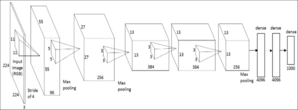
AlexNet architecture

When we look at the architecture, we can immediately see the input dimension 224 by 224 with three-dimensional depth. The stride size of four in the input, where max pooling layers are stacked, reduces the dimensionality of the input. In turn, this is followed by the convolutional layer. The two dense layers of size 4,096 are the fully connected layers leading to the final output that we mentioned before.

On a side note, we mentioned in a previous paragraph that TensorFlow's graph computation allows parallelization across GPUs. AlexNet did the same thing; look at the following image to see how they parallelized the architecture across GPUs:

The fully connected layer

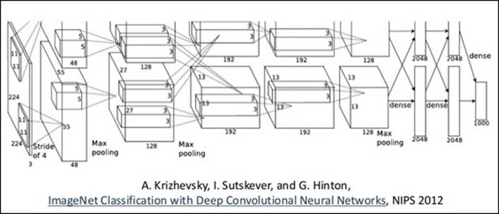
The preceding image is taken from http://www.cs.toronto.edu/~fritz/absps/imagenet.pdf.

AlexNet let different models utilize GPUs by splitting up the architecture vertically to later be merged into the final classification output. That CNNs are more suitable for distributed processing is one of the biggest advantages of locally connected networks over fully connected ones. This model trained a set of 1.2 million images and took five days to complete on two NVIDIA GTX 580 3GB GPUs. Two multiple GPU units (a total of six GPUs) were used for this project.

CNN's with an incremental approach

Now that we have a decent understanding of the architectures of CNNs, let's get our hands dirty in Keras and apply a CNN.

For this example, we will use the famous CIFAR-10 face image dataset, which is conveniently available within the Keras domain. The dataset consists of 60,000, 32 x 32 color images with 10 target classes consisting of an airplane, automobile, bird, cat, deer, dog, frog, horse, ship, and truck. This is a smaller dataset than the one that was used for the AlexNet example. For more information, you can refer to https://www.cs.toronto.edu/~kriz/cifar.html.

In this CNN, we will use the following architecture to classify the image according to the 10 classes that we specified:

input->convolution 1 (32,3,3)->convolution 2(32,3,3)->pooling->dropout -> Output (Fully connected layer and softmax)

GPU Computing

If you have a CUDA compatible graphics card installed, you can utilize your GPU for this CNN example by placing the following piece of code on top of your IDE:

import os

os.environ['THEANO_FLAGS'] = 'device=gpu0, assert_no_cpu_op=raise, on_unused_input=ignore, floatX=float32'

We do recommend however to first try this example on your regular CPU.

Let's first import and prepare the data.

We use a 32 x 32 input size considering this is the actual size of the image:

from keras.datasets import cifar10

from keras.preprocessing.image import ImageDataGenerator

from keras.models import Sequential

from keras.layers.core import Dense, Dropout, Activation, Flatten

from keras.layers.convolutional import Convolution2D, MaxPooling2D

from keras.optimizers import SGD

from keras.utils import np_utils

batch_size = 32

nb_classes = 10

nb_epoch = 5 #these are the number of epochs, watch out because it might set your #cpu/gpu on fire.

# input image dimensions

img_rows, img_cols = 32, 32

# the CIFAR10 images are RGB

img_channels = 3

# the data, shuffled and split between train and test sets

(X_train, y_train), (X_test, y_test) = cifar10.load_data()

print('X_train shape:', X_train.shape)

print(X_train.shape[0], 'train samples')

print(X_test.shape[0], 'test samples')

#remember we need to encode the target variable

Y_train = np_utils.to_categorical(y_train, nb_classes)

Y_test = np_utils.to_categorical(y_test, nb_classes)

Now let's setup our CNN architecture and construct the model according to the architecture we have in mind.

For this example, we will train our CNN model with vanilla SGD and Nesterov momentum:

model = Sequential()

#this is the first convolutional layer, we set the filter size

model.add(Convolution2D(32, 3, 3, border_mode='same',

input_shape=(img_channels, img_rows, img_cols)))

model.add(Activation('relu'))

#the second convolutional layer

model.add(Convolution2D(32, 3, 3))

model.add(Activation('relu'))

#here we specify the pooling layer

model.add(MaxPooling2D(pool_size=(2, 2)))

model.add(Dropout(0.25))

#first we flatten the input towards the fully connected layer into the softmax function

model.add(Flatten())

model.add(Dense(512))

model.add(Activation('relu'))

model.add(Dropout(0.2))

model.add(Dense(nb_classes))

model.add(Activation('softmax'))

# let's train the model using SGD + momentum like we have done before.

sgd = SGD(lr=0.01, decay=1e-6, momentum=0.9, nesterov=True)

model.compile(loss='categorical_crossentropy', optimizer=sgd)

X_train = X_train.astype('float32')

X_test = X_test.astype('float32')

#Here we apply scaling to the features

X_train /= 255

X_test /= 255

This step is very important because here we specify the CNN to train incrementally. We saw in previous chapters (refer to Chapter 2, Scalable Learning in Scikit-learn), and in a previous paragraph, the computational efficiency of online and incremental learning. We can mimic some of its properties and apply it to CNNs by using a very small epoch size with a smaller batch_size (fraction of the training set in each epoch), and train them incrementally in a for loop. This way, we can given the same amount of epochs and train our CNN in a much shorter time with also a lower burden on main memory. We can implement this very powerful idea with a simple for loop as follows:

for epoch in xrange(nb_epoch):

model.fit(X_train, Y_train, batch_size=batch_size, nb_epoch=1,show_accuracy=True

,validation_data=(X_test, Y_test), shuffle=True)

OUTPUT:]

X_train shape: (50000, 3, 32, 32)

50000 train samples

10000 test samples