Large Scale Machine Learning with Python (2016)

Chapter 6. Classification and Regression Trees at Scale

In this chapter, we will focus on scalable methods for classification and regression trees. The following topics will be covered:

· Tips and tricks for fast random forest applications in Scikit-learn

· Additive random forest models and subsampling

· GBM gradient boosting

· XGBoost together with streaming methods

· Very fast GBM and random forest in H2O

The aim of a decision tree is to learn a series of decision rules to infer the target labels based on the training data. Using a recursive algorithm, the process starts at the tree root and splits the data on the feature that results in the lowest impurity. Currently, the most widely applicable scalable tree-based applications are based on CART. Introduced by Breiman, Friedman Stone, and Ohlson in 1984, CART is an abbreviation of Classification and Regression Trees. CART is different from other decision tree models (such as ID3, C4.5/C5.0, CHAID, and MARS) in two ways. First, CART is applicable to both classification and regression problems. Second, it builds binary trees (at each split, resulting in a binary split). This enables CART trees to operate recursively on given features and optimize in a greedy fashion on an error metric in the form of impurity. These binary trees together with scalable solutions are the focus of this chapter.

Let's look closely at how these trees are constructed. We can see a decision tree as a graph with nodes, passing information down from top to bottom. Each decision within the tree is made by binary splits for either classes (Boolean) or continuous variables (a threshold value) resulting in a final prediction.

Trees are constructed and learned by the following procedure:

· Recursively finding the variable that best splits the target label from root to terminal node. This is measured by the impurity of each feature that we minimize based on the target outcome. In this chapter, the relevant impurity measures are Gini impurity and cross entropy.

Gini impurity

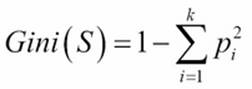
Gini impurity is a metric that measures the divergence between the probability pi of the target classes (k) so that an equal spread of probability values over the target classes result in a high Gini impurity.

Cross entropy

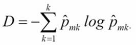
With cross entropy, we look at the log probability of misclassification. Both metrics are proven to yield quite similar results. However, Gini impurity is computationally more efficient because it does not require calculating the logs.

We do this until a stopping criterion is met. This criteria can roughly mean two things: one, adding new variables no longer improves the target outcome, and second, a maximum tree depth or tree complexity threshold is reached. Note that very deep and complex trees with many nodes can easily lead to overfitting. In order to prevent this, we generally prune the tree by limiting the tree depth.

To get an intuition for how this process works, let's build a decision tree with Scikit-learn and visualize it with graphviz. First, create a toy dataset to see if we can predict who is a smoker and who is not based on IQ (numeric), age (numeric), annual income (numeric), business owner (Boolean), and university degree (Boolean). You need to download the software from http://www.graphviz.org in order to load a visualization of the tree.dot file that we are going to create with Scikit-learn:

import numpy as np

from sklearn import tree

iq=[90,110,100,140,110,100]

age=[42,20,50,40,70,50]

anincome=[40,20,46,28,100,20]

businessowner=[0,1,0,1,0,0]

univdegree=[0,1,0,1,0,0]

smoking=[1,0,0,1,1,0]

ids=np.column_stack((iq, age, anincome,businessowner,univdegree))

names=['iq','age','income','univdegree']

dt = tree.DecisionTreeClassifier(random_state=99)

dt.fit(ids,smoking)

dt.predict(ids)

tree.export_graphviz(dt,out_file='tree2.dot',feature_names=names,label=all,max_depth=5,class_names=True)

You can now find the tree.dot file in your working directory. Once you find this file, you can open it with the graphviz software:

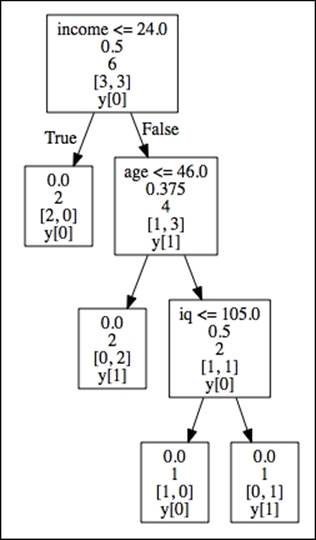
· Root node (Income): This is the starting node that represents the feature with the highest information gain and lowest impurity (Gini=.5)

· Internal nodes (Age and IQ):This is each node between the root node and terminal. Parent nodes pass down decision rules to the receiving end—child nodes (left and right)

· Terminal nodes (leaf nodes): The target labels partitioned by the tree structure

Tree-depth is the number of edges from the root node to the terminal nodes. In this case, we have a tree depth of 3.

We can now see all the binary splits resulting from the generated tree. At the top in the root node, we can see that a person with an income lower than 24k is not a smoker (income < 24). We can also see the corresponding Gini impurity (.5) for that split at each node. There are no left child nodes because the decision is final. The path simply ends there because it fully divides the target class. However, in the right child node (age) of income, the tree branches out. Here, if age is less than or equal to 46, then that person is not a smoker, but with an age older than 46 and an IQ lower than 105, that person is a smoker. Just as important are the few features we created that are not part of the tree—degree and business owner. This is because the variables in the tree are able to classify the target labels without them. These omitted features simply don't contribute to decreasing the impurity level of the tree.

Single trees have their drawbacks because they easily overtrain and therefore don't generalize well to unseen data. The current generation of these techniques are trained with ensemble methods where single trees are aggregated into much more powerful models. These CART ensemble techniques are one of the most used methods for machine learning because of their accuracy, ease of use, and capability to handle heterogeneous data. These techniques have been successfully applied in recent datascience competitions such as Kaggle and KDD-cup. As ensemble methods for classification and regression trees are currently the norm in the world of AI and data science, scalable solutions for CART-ensemble methods will be the main topic for this chapter.

Generally, we can discern two classes of ensemble methods that we use with CART models, namely bagging and boosting. Let's work through these concepts to form a better understanding of how the process of ensemble formation works.

Bootstrap aggregation

Bagging is an abbreviation of bootstrap aggregation. The bootstrapping technique originated in a context where analysts had to deal with a scarcity of data. With this statistical approach, subsamples were used to estimate population parameters when a statistical distribution couldn't be figured out a priori. The goal of bootstrapping is to provide a more robust estimate for population parameters where more variability is introduced to a smaller dataset by random subsampling with replacement. Generally, bootstrapping follows the following basic steps:

1. Randomly sample a batch of size x with replacement from a given dataset.

2. Calculate a metric or parameter from each sample to estimate the population parameters.

3. Aggregate the results.

In recent years, bootstrap methods have been used for parameters of machine learning models as well. An ensemble is most effective when its classifiers provide highly diverse decision boundaries. This diversity in ensembles can be achieved in the diversity of its underlying models and data these models are trained on. Trees are very well-suited for such diversity among classifiers because the structure of trees can be highly variable. However, the most popular method to ensemble is to use different training datasets to train individual classifiers. Often, such datasets are obtained through subsampling-sampling techniques, such as bootstrapping and bagging. Everything started from the idea that by leveraging more data, we can reduce the variance of the estimates. If it is not possible to have more data at hand, resampling can provide a significant improvement because it allows retraining the algorithm over many versions of the training sample. This is where the idea of bagging comes in; using bagging, we take the original bootstrap idea a bit further by aggregation (averaging, for instance) of the results of many resamples in order to arrive at a final prediction where the errors due to in-sample overfitting are reciprocally smoothed out.

When we apply an ensemble technique such as bagging to tree models, we build multiple trees on each separate bootstrapped sample (or subsampled using sampling without replacement) of the original dataset and then aggregate the results (usually by arithmetic, geometric averaging, or voting).

In such a fashion, a standard bagging algorithm will look as follows:

1. Draw an n amount of random samples with size K with replacement from the full dataset (S1, S2, … Sn).

2. Train distinct trees on (S1, S2, … Sn).

3. Calculate predictions on samples (S1, S2, … Sn) on new data and aggregate their results.

CART models benefit very well from bagging methods because of the stochasticity and diversity it introduces.

Random forest and extremely randomized forest

Apart from bagging, based on training examples, we can also draw random subsamples based on features. Such a method is referred to as Random Subspaces. Random subspaces are particularly useful for high-dimensional data (data with lots of features) and it is the foundation of the method that we refer to as random forest. At the time of writing this, random forest is the most popular machine learning algorithm because of its ease of use, robustness to messy data, and parallelizability. It found its way into all sorts of applications such as location apps, games, and screening methods for healthcare applications. For instance, the Xbox Kinect uses a random forest model for motion detection purposes. Considering that the random forest algorithm is based on bagging methods, the algorithm is relatively straightforward:

1. Bootstrap m samples of size N from the available sample.

2. Trees are constructed independently on each subset (S1, S2, … Sn) using a different fraction of the feature set G (without replacement) at every node split.

3. Minimize the error of the node splits (based on the Gini index or entropy measure).

4. Have each tree make a prediction and aggregate the results, using voting for classification and averaging for regression.

As bagging relies on multiple subsamples, it's an excellent candidate for parallelization where each CPU unit is dedicated to calculating separate models. In this way, we can speed up the learning using the widespread availability of multiple cores. As a limit in such a scaling strategy, we have to be aware that Python is single-threaded and we will have to replicate many Python instances, each replicating the memory space with the in-sample examples we have to employ. Consequently, we will need to have a lot of RAM memory available in order to fit the training matrix and the number of processes. If the available RAM does not suffice, setting the number of parallel tree computations running at once on our computer will not help scaling the algorithm. In this case, CPU usage and RAM memory are important bottlenecks.

Random forests models are quite easy to employ for machine learning because they don't require a lot of hyperparameter tuning to perform well. The most important parameters of interest are the amount of trees and depth of the trees (tree depth) that have the most influence on the performance of the model. When operating on these two hyperparameters, it results in an accuracy/performance trade-off where more trees and more depth lead to higher computational load. Our experience as practitioners suggests not to set the value of the amount of trees too high because eventually, the model will reach a plateau in performance and won't improve anymore when adding more trees but will just result in taxing the CPU cores. Under such considerations, although a random forest model with default parameters performs well just out of the box, we can still increase its performance by tuning the number of trees. See the following table for an overview of the hyperparameters for random forests.

The most important parameters for bagging with a random forest:

· n_estimators: The number of trees in the model

· max_features: The number of features used for tree construction

· min_sample_leaf: Node split is removed if a terminal node contains less samples than the minimum

· max_depth: The number of nodes that we pass top-down from the root to the terminal node

· criterion: The method used to calculate the best split (Gini or entropy)

· min_samples_split: The minimum number of samples required to split an internal node

Scikit-learn provides a wide range of powerful CART ensemble applications, some of which are quite computationally efficient. When it comes to random forests, there is an often-overlooked algorithm called extra-trees, better known as Extremely Randomized Forest. When it comes to CPU efficiency, extra-trees can deliver a considerable speedup from regular random forests—sometimes even in tenfolds.

In the following table, you can see the computation speed for each method. Extra-trees is considerably faster with a more pronounced difference once we increase the sample size:

Models were trained with 50 features and 100 estimators for both extra trees and random forest. We used a quad-core MacBook Pro with 16GB RAM for this example. We measured the training time in seconds.

In this paragraph, we will use extreme forests instead of the vanilla random forest method in Scikit-learn. So you might ask: how are they different? The difference is not strikingly complex. In random forests, the node split decision rules are based on a best score resulting from the randomly selected features at each iteration. In extremely randomized forests, a random split is generated on each feature in the random subset (so there are no computations spent on looking for the best split for each feature) and then the best scoring threshold is selected. Such an approach brings about some advantageous properties because the method leads to achieving models with lower variance even if each individual tree is grown until having the greatest possible accuracy in terminal nodes. As more randomness is added to branch splits, the tree learner makes errors, which are consequently less correlated among the trees in the ensemble. This will lead to much more uncorrelated estimations in the ensemble and, depending on the learning problem (there is no free lunch, after all), to a lower generalization error than a standard random forest ensemble. In practice, however, a regular random forest model can provide a slightly higher accuracy.

Given such interesting learning properties, with a more efficient node split calculation and the same parallelism that can be leveraged for random forests, we consider extremely randomized trees as an excellent candidate in the range of ensemble tree algorithms, if we want to speed up in-core learning.

To read a detailed description of the extremely randomized forest algorithm, you can read the following article that started everything:

P. Geurts, D. Ernst, and L. Wehenkel, Extremely randomized trees, Machine Learning, 63(1), 3-42, 2006. This article can be freely accessed at https://www.semanticscholar.org/paper/Extremely-randomized-trees-Geurts-Ernst/336a165c17c9c56160d332b9f4a2b403fccbdbfb/pdf.

As an example of how to scale in-core tree ensembles, we will run an example where we apply an efficient random forest method to credit data. This dataset is used to predict credit card clients' default rates. The data consists of 18 features and 30,000 training examples. As we need to import a file in XLS format, you will need to install the xlrd package, and we can achieve this by typing the following in the command-line terminal:

$ pip install xlrd

import pandas as pd

import numpy as np

import os

import xlrd

import urllib

#set your path here

os.chdir('/your-path-here')

url = 'http://archive.ics.uci.edu/ml/machine-learning-databases/00350/default%20of%20credit%20card%20clients.xls'

filename='creditdefault.xls'

urllib.urlretrieve(url, filename)

target = 'default payment next month'

data = pd.read_excel('creditdefault.xls', skiprows=1)

target = 'default payment next month'

y = np.asarray(data[target])

features = data.columns.drop(['ID', target])

X = np.asarray(data[features])

from sklearn.ensemble import ExtraTreesClassifier

from sklearn.cross_validation import cross_val_score

from sklearn.datasets import make_classification

from sklearn.cross_validation import train_test_split

X_train, X_test, y_train, y_test = train_test_split(X, y,test_size=0.30, random_state=101)

clf = ExtraTreesClassifier(n_estimators=500, random_state=101)

clf.fit(X_train,y_train)

scores = cross_val_score(clf, X_train, y_train, cv=3,scoring='accuracy', n_jobs=-1)

print "ExtraTreesClassifier -> cross validation accuracy: mean = %0.3f std = %0.3f" % (np.mean(scores), np.std(scores))

Output]

ExtraTreesClassifier -> cross validation accuracy: mean = 0.812 std = 0.003

Now that we have some base estimation of the accuracy on the training set, let's see how well it performs on the test set. In this case, we want to monitor the false positives and false negatives and also check for class imbalances on the target variable:

y_pred=clf.predict(X_test)

from sklearn.metrics import confusion_matrix

confusionMatrix = confusion_matrix(y_test, y_pred)

print confusionMatrix

from sklearn.metrics import accuracy_score

accuracy_score(y_test, y_pred)

OUTPUT:

[[6610 448]

[1238 704]]

Our overall test accuracy:

0.81266666666666665

Interestingly, the test set accuracy is equal to our training results. As our baseline model is just using the default setting, we can try to improve performance by tuning the hyperparameters, a task that can be computationally expensive. Recently, more computationally efficient methods have been developed for hyperparameter optimization, which we will cover in the next section.

Fast parameter optimization with randomized search

You might already be familiar with Scikit-learn's gridsearch functionalities. It is a great tool but when it comes to large files, it can ramp up training time enormously depending on the parameter space. For extreme random forests, we can speed up the computation time for parameter tuning using an alternative parameter search method named randomized search. Where common gridsearch taxes both CPU and memory by systematically testing all possible combinations of the hyperparameter settings, randomized search selects combinations of hyperparameters at random. This method can lead to a considerable computational speedup when the gridsearch is testing more than 30 combinations (for smaller search spaces, gridsearch is still competitive). The gain achievable is in the same order as we have seen when we switched from random forests to extremely randomized forests (think between a two to tenfold gain, depending on hardware specifications, hyperparameter space, and the size of the dataset).

We can specify the number of hyperparameter settings that are evaluated randomly by the n_iter parameter:

from sklearn.grid_search import GridSearchCV, RandomizedSearchCV

param_dist = {"max_depth": [1,3, 7,8,12,None],

"max_features": [8,9,10,11,16,22],

"min_samples_split": [8,10,11,14,16,19],

"min_samples_leaf": [1,2,3,4,5,6,7],

"bootstrap": [True, False]}

#here we specify the search settings, we use only 25 random parameter

#valuations but we manage to keep training times in check.

rsearch = RandomizedSearchCV(clf, param_distributions=param_dist,

n_iter=25)

rsearch.fit(X_train,y_train)

rsearch.grid_scores_

bestclf=rsearch.best_estimator_

print bestclf

Here, we can see the list of optimal parameter settings for our model.

We can now use this model to make predictions on our test set:

OUTPUT:

ExtraTreesClassifier(bootstrap=False, class_weight=None, criterion='gini',

max_depth=12, max_features=11, max_leaf_nodes=None,

min_samples_leaf=4, min_samples_split=10,

min_weight_fraction_leaf=0.0, n_estimators=500, n_jobs=1,

oob_score=False, random_state=101, verbose=0, warm_start=False)

y_pred=bestclf.predict(X_test)

confusionMatrix = confusion_matrix(y_test, y_pred)

print confusionMatrix

accuracy=accuracy_score(y_test, y_pred)

print accuracy

OUT

[[6733 325]

[1244 698]]

Out[152]:

0.82566666666666666

We managed to increase the performance of our model within a manageable range of training time and increase accuracy at the same time.

Extremely randomized trees and large datasets

So far, we have looked at solutions to scale up leveraging multicore CPUs and randomization thanks to the specific characteristics of random forest and its more efficient alternative, extremely randomized forest. However, if you have to deal with a large dataset that won't fit in memory or is too CPU-demanding, you may want to try an out-of-core solution. The best solution for an out-of-core approach with ensembles is the one provided by H2O, which will be covered in detail later in this chapter. However, we can exert another practical trick in order to have random forest or extra-trees running smoothly on a large-scale dataset. A second-best solution would be to train models on subsamples of the data and then ensemble the results from each model built on different subsamples of the data (after all, we just have to average or group the results). In Chapter 3, Fast-Learning SVMs, we already introduced the concept of reservoir sampling, dealing with sampling on data streams. In this chapter, we will use sampling again, resorting to a larger choice of sampling algorithms. First, let's install a really handy tool called subsample developed by Paul Butler (https://github.com/paulgb/subsample), a command-line tool to sample data from a large, newline-separated dataset (typically, a CSV-like file). This tool provides quick and easy sampling methods such as reservoir sampling.

As seen in Chapter 3, Fast-Learning SVMs, reservoir sampling is a sampling algorithm that helps sampling fixed-size samples from a stream. Conceptually simple (we have seen the formulation in Chapter 3), it just needs a simple pass over the data to produce a sample that will be stored in a new file on disk. (Our script in Chapter 3 stored it in memory, instead.)

In the next example, we will use this subsample tool together with a method to ensemble the models trained on these subsamples.

To recap, in this section, we are going to perform the following actions:

1. Create our dataset and split it into test and training data.

2. Draw subsamples of the training data and save them as separate files on our harddrive.

3. Load these subsamples and train extremely randomized forest models on them.

4. Aggregate the models.

5. Check the results.

Let's install this subsample tool with pip:

$pip install subsample

In the command line, set the working directory containing the file that you want to sample:

$ cd /yourpath-here

At this point, using the cd command, you can specify your working directory where you will need to store the file that we will create in the next step.

We do this in the following way:

from sklearn.datasets import fetch_covtype

import numpy as np

from sklearn.cross_validation import train_test_split

dataset = fetch_covtype(random_state=111, shuffle=True)

dataset = fetch_covtype()

X, y = dataset.data, dataset.target

X_train, X_test, y_train, y_test = train_test_split(X,y, test_size=0.3, random_state=0)

del(X,y)

covtrain=np.c_[X_train,y_train]

covtest=np.c_[X_test,y_test]

np.savetxt('covtrain.csv', covtrain, delimiter=",")

np.savetxt('covtest.csv', covtest, delimiter=",")

Now that we have split the dataset into test and training sets, let's subsample the training set in order to obtain chunks of data that we can manage to upload in-memory. Considering that the size of the full training dataset is 30,000 examples, we will subsample three smaller datasets, each one made of 10,000 items. If you have a computer equipped with less than 2GB of RAM memory, you may find it more manageable to split the initial training set into smaller files, though the modeling results that you will obtain will likely differ from our example based on three subsamples. As a rule, the fewer the examples in the subsamples, the greater will be the bias of your model. When subsampling, we are actually trading the advantage of working on a more manageable amount of data against an increased bias of the estimates:

$ subsample --reservoir -n 10000 covtrain.csv > cov1.csv

$ subsample --reservoir -n 10000 covtrain.csv > cov2.csv

$ subsample --reservoir -n 10000 covtrain.csv>cov3.csv

You can now find these subsets in the folder that you specified in the command line.

Now make sure that you set the same path in your IDE or notebook.

Let's load the samples one by one and train a random forest model on them.

To combine them later for a final prediction, note that we keep a single line-by-line approach so that you can follow the consecutive steps closely.

In order for these examples to be successful, make sure that you are working on the same path set in your IDE or Jupyter Notebook:

import os

os.chdir('/your-path-here')

At this point, we are ready to start learning from the data and we can load the samples in-memory one by one and train an ensemble of trees on them:

import numpy as np

from sklearn.ensemble import ExtraTreesClassifier

from sklearn.cross_validation import cross_val_score

from sklearn.cross_validation import train_test_split

import pandas as pd

import os

After reporting a validation score, the code will proceed training our model on all the data chunks, one at a time. As we are learning separately from different data partitions, data chunk after data chunk, we initialize the ensemble learner (in this case,ExtraTreeClassifier) using the warm_start=Trueparameter and set_params method that incrementally adds trees from the previous training sessions as the fit method is called multiple times:

#here we load sample 1

df = pd.read_csv('/yourpath/cov1.csv')

y=df[df.columns[54]]

X=df[df.columns[0:54]]

clf1=ExtraTreesClassifier(n_estimators=100, random_state=101,warm_start=True)

clf1.fit(X,y)

scores = cross_val_score(clf1, X, y, cv=3,scoring='accuracy', n_jobs=-1)

print "ExtraTreesClassifier -> cross validation accuracy: mean = %0.3f std = %0.3f" % (np.mean(scores), np.std(scores))

print scores

print 'amount of trees in the model: %s' % len(clf1.estimators_)

#sample 2

df = pd.read_csv('/yourpath/cov2.csv')

y=df[df.columns[54]]

X=df[df.columns[0:54]]

clf1.set_params(n_estimators=150, random_state=101,warm_start=True)

clf1.fit(X,y)

scores = cross_val_score(clf1, X, y, cv=3,scoring='accuracy', n_jobs=-1)

print "ExtraTreesClassifier after params -> cross validation accuracy: mean = %0.3f std = %0.3f" % (np.mean(scores), np.std(scores))

print scores

print 'amount of trees in the model: %s' % len(clf1.estimators_)

#sample 3

df = pd.read_csv('/yourpath/cov3.csv')

y=df[df.columns[54]]

X=df[df.columns[0:54]]

clf1.set_params(n_estimators=200, random_state=101,warm_start=True)

clf1.fit(X,y)

scores = cross_val_score(clf1, X, y, cv=3,scoring='accuracy', n_jobs=-1)

print "ExtraTreesClassifier after params -> cross validation accuracy: mean = %0.3f std = %0.3f" % (np.mean(scores), np.std(scores))

print scores

print 'amount of trees in the model: %s' % len(clf1.estimators_)

# Now let's predict our combined model on the test set and check our score.

df = pd.read_csv('/yourpath/covtest.csv')

X=df[df.columns[0:54]]

y=df[df.columns[54]]

pred2=clf1.predict(X)

scores = cross_val_score(clf1, X, y, cv=3,scoring='accuracy', n_jobs=-1)

print "final test score %r" % np.mean(scores)

OUTPUT:]

ExtraTreesClassifier -> cross validation accuracy: mean = 0.803 std = 0.003

[ 0.805997 0.79964007 0.8021021 ]

amount of trees in the model: 100

ExtraTreesClassifier after params -> cross validation accuracy: mean = 0.798 std = 0.003

[ 0.80155875 0.79651861 0.79465626]

amount of trees in the model: 150

ExtraTreesClassifier after params -> cross validation accuracy: mean = 0.798 std = 0.006

[ 0.8005997 0.78974205 0.8033033 ]

amount of trees in the model: 200

final test score 0.92185447181058278

Note

Warning: This method looks un-Pythonic but is quite effective.

We have improved the score on the final prediction now; we went from an accuracy of around .8 to an accuracy of .922 on the test set. This is because we have a final combined model containing all the tree information combined of the previous three random forest models. In the code's output, you can also notice the number of trees that are added to the initial model.

From here, you might want to try such an approach on even larger datasets leveraging more subsamples, or apply randomized search to one of the subsamples for better tuning.

CART and boosting

We started this chapter with bagging; now we will complete our overview with boosting, a different ensemble method. Just like bagging, boosting can be used for both regression and classification and has recently overshadowed random forest for higher accuracy.

As an optimization process, boosting is based on the stochastic gradient descent principle that we have seen in other methods, namely optimizing models by minimizing error according to gradients. The most familiar boosting methods to date are AdaBoost and Gradient Boosting (GBM and recently XGBoost). The AdaBoost algorithm comes down to minimizing the error of those cases where the prediction is slightly wrong so that cases that are harder to classify get more attention. Recently, AdaBoost fell out of favor as other boosting methods were found to be generally more accurate.

In this chapter, we will cover the two most effective boosting algorithms available to date to Python users: Gradient Boosting Machine (GBM) found in the Scikit-learn package and extreme gradient boosting (XGBoost). As GBM is sequential in nature, the algorithm is hard to parallelize and thus harder to scale than random forest, but some tricks will do the job. Some tips and tricks to speed up the algorithm will be covered with a nice out-of-memory solution for H2O.

Gradient Boosting Machines

As we have seen in the previous sections, random forests and extreme trees are efficient algorithms and both work quite well with minimum effort. Though recognized as a more accurate method, GBM is not very easy to use and it is always necessary to tune its many hyperparameters in order to achieve the best results. Random forest, on the other hand, can perform quite well with only a few parameters to consider (mostly tree depth and number of trees). Another thing to pay attention to is overtraining. Random forests are less sensitive to overtraining than GBM. So, with GBM, we also need to think about regularization strategies. Above all, random forests are much easier to perform parallel operations where as GBM is sequential and thus slower to compute.

In this chapter, we will apply GBM in Scikit-learn, look at the next generation of tree boosting algorithms named XGBoost, and implement boosting on a larger scale on H2O.

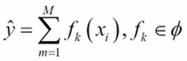
The GBM algorithm that we use in Scikit-learn and H2O is based on two important concepts: additive expansion and gradient optimization by the steepest descent algorithm. The general idea of the former is to generate a sequence of relatively simple trees (weak learners), where each successive tree is added along a gradient. Let's assume that we have M trees that aggregate the final predictions in the ensemble. The tree in each iteration fk is now part of a much broader space of all the possible trees in the model () (in Scikit-learn, this parameter is better known as n_estimators):

The additive expansion will add new trees to previous trees in a stage-wise manner:

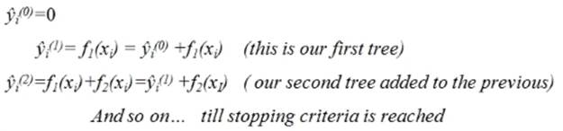
The prediction of our gradient boosting ensemble is simply the sum of the predictions of all the previous trees and the newly added tree , more formally leading to the following:

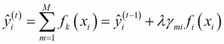
The second important and yet quite tricky part of the GBM algorithm is gradient optimization by steepest descent. This means that we add increasingly more powerful trees to the additive model. This is achieved by applying gradient optimization to the new trees. How do we perform gradient updates with trees as there are no parameters like we have seen with traditional learning algorithms? First, we parameterize the trees; we do this by recursively upgrading the node split values along a gradient where the nodes are represented by a vector. This way, the steepest descent direction is the negative gradient of the loss function and the node splits will be upgraded and learned, leading to:

· : A shrinkage parameter (also referred to as learning rate in this context) that will cause the ensemble to learn slowly with the addition of more trees

· : The gradient upgrade parameter also referred to as the step length

The prediction score for each leaf is thus the final score for the new tree that then simply is the sum over each leaf:

So to summarize, GBM works by incrementally adding more accurate trees learned along the gradient.

Now that we understand the core concepts, let's run a GBM example and look at the most important parameters. For GBM, these parameters are extra important because when we set this number of trees too high, we are bound to strain our computational resources exponentially. So be careful with these parameters. Most parameters in Scikit-learn's GBM application are the same as in random forest, which we have covered in the previous paragraph. There are three parameters that we need to take into account that need special attention.

max_depth

Contrary to random forests, which perform better when they build their tree structures to their maximum extension (thus building and ensembling predictors with high variance), GBM tends to work better with smaller trees (thus leveraging predictors with a higher bias, that is, weak learners). Working with smaller decision trees or just with stumps (decision trees with only one single branch) can alleviate the training time, trading off the speediness of execution against a larger bias (because a smaller tree can hardly intercept more complex relationships in data).

learning_rate

Also known as shrinkage , this is a parameter related to the gradient descent optimization and how each tree will contribute to the ensemble. Smaller values of this parameter can improve the optimization in the training process, though it will require more estimators to converge and thus more computational time. As it affects the weight of each tree in the ensemble, smaller values imply that each tree will contribute a small part to the optimization process and you will need more trees before reaching a good solution. Consequently, when optimizing this parameter for performance, we should avoid too large values that may lead to sub-optimal models; we also have to avoid using too low values because this will affect the computation time heavily (more trees will be needed for the ensemble to converge to a solution). In our experience, a good starting point is to use a learning rate in the range <0.1 and >.001.

Subsample

Let's recall the principles of bagging and pasting, where we take random samples and construct trees on those samples. If we apply subsampling to GBM, we randomize the tree constructions and prevent overfitting, reduce memory load, and even sometimes increase accuracy. We can apply this procedure to GBM as well, making it more stochastic and thus leveraging the advantages of bagging. We can randomize the tree construction in GBM by setting the subsample parameter to .5.

Faster GBM with warm_start

This parameter allows storing new tree information after each iteration is added to the previous one without generating new trees. This way, we can save memory and speed up computation time extensively.

Using the GBM available in Scikit-learn, there are two actions that we can take in order to increase memory and CPU efficiency:

· Warm start for (semi) incremental learning

· We can use parallel processing during cross-validation

Let's run through a GBM classification example where we use the spam dataset from the UCI machine learning library. We will first load the data, preprocess it, and look at the variable importance of each feature:

import pandas

import urllib2

import urllib2

from sklearn import ensemble

columnNames1_url = 'https://archive.ics.uci.edu/ml/machine-learning-databases/spambase/spambase.names'

columnNames1 = [

line.strip().split(':')[0]

for line in urllib2.urlopen(columnNames1_url).readlines()[33:]]

columnNames1

n = 0

for i in columnNames1:

columnNames1[n] = i.replace('word_freq_','')

n += 1

print columnNames1

spamdata = pandas.read_csv(

'https://archive.ics.uci.edu/ml/machine-learning-databases/spambase/spambase.data',

header=None, names=(columnNames1 + ['spam'])

)

X = spamdata.values[:,:57]

y=spamdata['spam']

spamdata.head()

import numpy as np

from sklearn import cross_validation

from sklearn.metrics import classification_report

from sklearn.cross_validation import cross_val_score

from sklearn.cross_validation import cross_val_predict

from sklearn.cross_validation import train_test_split

from sklearn.metrics import recall_score, f1_score

from sklearn.cross_validation import cross_val_predict

import matplotlib.pyplot as plt

from sklearn.metrics import confusion_matrix

from sklearn.metrics import accuracy_score

from sklearn.ensemble import GradientBoostingClassifier

X_train, X_test, y_train, y_test = train_test_split(X,y, test_size=0.3, random_state=22)

clf = ensemble.GradientBoostingClassifier(n_estimators=300,random_state=222,max_depth=16,learning_rate=.1,subsample=.5)

scores=clf.fit(X_train,y_train)

scores2 = cross_val_score(clf, X_train, y_train, cv=3, scoring='accuracy',n_jobs=-1)

print scores2.mean()

y_pred = cross_val_predict(clf, X_test, y_test, cv=10)

print 'validation accuracy %s' % accuracy_score(y_test, y_pred)

OUTPUT:]

validation accuracy 0.928312816799

confusionMatrix = confusion_matrix(y_test, y_pred)

print confusionMatrix

from sklearn.metrics import accuracy_score

accuracy_score(y_test, y_pred)

clf.feature_importances_

def featureImp_order(clf, X, k=5):

return X[:,clf.feature_importances_.argsort()[::-1][:k]]

newX = featureImp_order(clf,X,2)

print newX

# let's order the features in amount of importance

print sorted(zip(map(lambda x: round(x, 4), clf.feature_importances_), columnNames1),

reverse=True)

OUTPUT]

0.945030177548

precision recall f1-score support

0 0.93 0.96 0.94 835

1 0.93 0.88 0.91 546

avg / total 0.93 0.93 0.93 1381

[[799 36]

[ 63 483]]

Feature importance:

[(0.2262, 'char_freq_;'),

(0.0945, 'report'),

(0.0637, 'capital_run_length_average'),

(0.0467, 'you'),

(0.0461, 'capital_run_length_total')

(0.0403, 'business')

(0.0397, 'char_freq_!')

(0.0333, 'will')

(0.0295, 'capital_run_length_longest')

(0.0275, 'your')

(0.0259, '000')

(0.0257, 'char_freq_(')

(0.0235, 'char_freq_$')

(0.0207, 'internet')

We can see that the character ; is the most discriminative in classifying spam.

Note

Variable importance shows us how much splitting each feature reduces the relative impurity across all the splits in the tree.

Speeding up GBM with warm_start

Unfortunately, there is no parallel processing for GBM in Scikit-learn. Only cross-validation and gridsearch can be parallelized. So what can we do to make it faster? We saw that GBM works with the principle of additive expansion where trees are added incrementally. We can utilize this idea in Scikit-learn with the warm-start parameter. We can model this with Scikit-learn's GBM functionalities by building tree models incrementally with a handy for loop. So let's do this with the same dataset and inspect the computational advantage that it provides:

gbc = GradientBoostingClassifier(warm_start=True, learning_rate=.05, max_depth=20,random_state=0)

for n_estimators in range(1, 1500, 100):

gbc.set_params(n_estimators=n_estimators)

gbc.fit(X_train, y_train)

y_pred = gbc.predict(X_test)

print(classification_report(y_test, y_pred))

print(gbc.set_params)

OUTPUT:

precision recall f1-score support

0 0.93 0.95 0.94 835

1 0.92 0.89 0.91 546

avg / total 0.93 0.93 0.93 1381

<bound method GradientBoostingClassifier.set_params of GradientBoostingClassifier(init=None, learning_rate=0.05, loss='deviance',

max_depth=20, max_features=None, max_leaf_nodes=None,

min_samples_leaf=1, min_samples_split=2,

min_weight_fraction_leaf=0.0, n_estimators=1401,

presort='auto', random_state=0, subsample=1.0, verbose=0,

warm_start=True)>

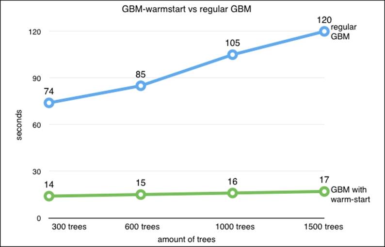
It's adviable to pay special attention to the output of the settings of the tree (n_estimators=1401). You can see that the size of the tree we used is 1401. This little trick helped us reduce the training time a lot (think half or even less) when we compare it to a similar GBM model, which we would have trained with 1401 trees at once. Note that we can use this method for random forest and extreme random forest as well. Nevertheless, we found this useful specifically for GBM.

Let's look at the figure that shows the training time for a regular GBM and our warm_start method. The computation speedup is considerable with the accuracy remaining relatively the same:

Training and storing GBM models

Ever thought of training a model on three computers at the same time? Or training a GBM model on an EC2 instance? There might be a case where you train a model and want to store it to use it again later on. When you have to wait for two days for a full training round to complete, we don't want to have to go through that process again. A case where you have trained a model in the cloud on an Amazon EC2 instance, you can store that model and reuse it later on another computer using Scikit-learn's joblib. So let's walk through this process as Scikit-learn has provided us with a handy tool to manage it.

Let's import the right libraries and set our directories for our file locations:

import errno

import os

#set your path here

path='/yourpath/clfs'

clfm=os.makedirs(path)

os.chdir(path)

Now let's export the model to the specified location on our harddrive:

from sklearn.externals import joblib

joblib.dump( gbc,'clf_gbc.pkl')

Now we can load the model and reuse it for other purposes:

model_clone = joblib.load('clf_gbc.pkl')

zpred=model_clone.predict(X_test)

print zpred

XGBoost

We have just discussed that there are no options for parallel processing when using GBM from Scikit-learn, and this is exactly where XGBoost comes in. Expanding on GBM, XGBoost introduces more scalable methods leveraging multithreading on a single machine and parallel processing on clusters of multiple servers (using sharding). The most important improvement of XGBoost over GBM lies in the capability of the latter to manage sparse data. XGBoost automatically accepts sparse data as input without storing zero values in memory. A second benefit of XGBoost lies in the way in which the best node split values are calculated while branching the tree, a method named quantile sketch. This method transforms the data by a weighting algorithm so that candidate splits are sorted based on a certain accuracy level. For more information read the article at http://arxiv.org/pdf/1603.02754v3.pdf.

XGBoost stands for Extreme Gradient Boosting, an open source gradient boosting algorithm that has gained a lot of popularity in data science competitions such as Kaggle (https://www.kaggle.com/) and KDD-cup 2015. (The code is available on GitHub athttps://github.com/dmlc/XGBoost, as we described in Chapter 1, First Steps to Scalability.) As the authors (Tianqui Chen, Tong He, and Carlos Guestrin) report on papers that they wrote on their algorithm, XGBoost, among 29 challenges held on Kaggle during 2015, 17 winning solutions used XGBoost as a standalone or part of some kind of ensemble of multiple models. In their paper XGBoost: A Scalable Tree Boosting System (which can be found at http://learningsys.org/papers/LearningSys_2015_paper_32.pdf), the authors report that, in the recent KDD-cup 2015, XGBoost was used by every team that ended in the top ten of the competition. Apart from successful performances in both accuracy and computational efficiency, our principal concern in this book is scalability, and XGBoost is indeed a scalable solution from different points of view. XGBoost is a new generation of GBM algorithms with important tweaks to the initial tree boost GBM algorithm. XGBoost provides parallel processing; the scalability offered by the algorithm is due to quite a few new tweaks and additions developed by its authors:

· An algorithm that accepts sparse data, which can leverage sparse matrices, saving both memory (no need for dense matrices) and computation time (zero values are handled in a special way)

· An approximate tree learning (weighted quantile sketch), which bears similar results but in much less time than the classical complete explorations of possible branch cuts

· Parallel computing on a single machine (using multithreading in the phase of the search for the best split) and similarly distributed computations on multiple ones

· Out-of-core computations on a single machine leveraging a data storage solution called Column Block, which arranges data on disk by columns, thus saving time by pulling data from disk as the optimization algorithm (which works on column vectors) expects it

From a practical point of view, XGBoost features mostly the same parameters as GBM. XGBoost is also quite capable of dealing with missing data. Other tree ensembles, based on standard decisions trees, require missing data first to be imputed using an off-scale value (such as a large negative number) in order to develop an appropriate branching of the tree to deal with missing values. XGBoost, instead, first fits all the non-missing values and, after having created the branching for the variable, it decides which branch is better for the missing values to take in order to minimize the prediction error. Such an approach leads to trees that are more compact and an effective imputation strategy leading to more predictive power.

The most important XGBoost parameters are as follows:

· eta (default=0.3): This is the equivalent of the learning rate in Scikit-learn's GBM

· min_child_weight (default=1): Higher values prevent overfitting and tree complexity

· max_depth (default=6): This is the number of interactions in the trees

· subsample (default=1): This is a fraction of samples of the training data that we take in each iteration

· colsample_bytree (default=1): This is the fraction of features in each iteration

· lambda (default=1): This is the L2 regularization (Boolean)

· seed (default=0): This is the equivalent of Scikit-learn's random_state parameter, allowing reproducibility of learning processes across multiple tests and different machines

Now that we know XGBoost's most important parameters, let's run an XGBoost example on the same dataset that we used for GBM with the same parameter settings (as much as possible). XGBoost is a little less straightforward to use than the Scikit-learn package. So we will provide some basic examples that you can use as a starting point for more complex models. Before we dive deeper into XGBoost applications, let's compare it to the GBM method in sklearn on the spam dataset; we have already loaded the data in-memory:

import xgboost as xgb

import numpy as np

from sklearn.metrics import classification_report

from sklearn import cross_validation

clf = xgb.XGBClassifier(n_estimators=100,max_depth=8,

learning_rate=.1,subsample=.5)

clf1 = GradientBoostingClassifier(n_estimators=100,max_depth=8,

learning_rate=.1,subsample=.5)

%timeit xgm=clf.fit(X_train,y_train)

%timeit gbmf=clf1.fit(X_train,y_train)

y_pred = xgm.predict(X_test)

y_pred2 = gbmf.predict(X_test)

print 'XGBoost results %r' % (classification_report(y_test, y_pred))

print 'gbm results %r' % (classification_report(y_test, y_pred2))

OUTPUT:

1 loop, best of 3: 1.71 s per loop

1 loop, best of 3: 2.91 s per loop

XGBoost results ' precision recall f1-score support\n\n 0 0.95 0.97 0.96 835\n 1 0.95 0.93 0.94 546\n\navg / total 0.95 0.95 0.95 1381\n'

gbm results ' precision recall f1-score support\n\n 0 0.95 0.97 0.96 835\n 1 0.95 0.92 0.93 546\n\navg / total 0.95 0.95 0.95 1381\n

We can clearly see that XGBoost is quite faster than GBM (1.71s versus 2.91s) even though we didn't use parallelization for XGBoost. Later, we can even arrive at a greater speedup when we use parallelization and out-of-core methods for XGBoost when we apply out-of-memory streaming. In some cases, the XGBoost model results in a higher accuracy than GBM, but (almost) never the other way around.

XGBoost regression

Boosting methods are often used for classification but can be very powerful for regression tasks as well. As regression is often overlooked, let's run a regression example and walk through the key issues. Let's fit a boosting model on the California housing set with gridsearch. The California house dataset has recently been added to Scikit-learn, which saves us some preprocessing steps:

import numpy as np

import scipy.sparse

import xgboost as xgb

import os

import pandas as pd

from sklearn.cross_validation import train_test_split

import numpy as np

from sklearn.datasets import fetch_california_housing

from sklearn.metrics import mean_squared_error

pd=fetch_california_housing()

#because the y variable is highly skewed we apply the log transformation

y=np.log(pd.target)

X_train, X_test, y_train, y_test = train_test_split(pd.data,

y,

test_size=0.15,

random_state=111)

names = pd.feature_names

print names

import xgboost as xgb

from xgboost.sklearn import XGBClassifier

from sklearn.grid_search import GridSearchCV

clf=xgb.XGBRegressor(gamma=0,objective= "reg:linear",nthread=-1)

clf.fit(X_train,y_train)

y_pred = clf.predict(X_test)

print 'score before gridsearch %r' % mean_squared_error(y_test, y_pred)

params = {

'max_depth':[4,6,8],

'n_estimators':[1000],

'min_child_weight':range(1,3),

'learning_rate':[.1,.01,.001],

'colsample_bytree':[.8,.9,1]

,'gamma':[0,1]}

#with the parameter nthread we specify XGBoost for parallelisation

cvx = xgb.XGBRegressor(objective= "reg:linear",nthread=-1)

clf=GridSearchCV(estimator=cvx,param_grid=params,n_jobs=-1,scoring='mean_absolute_error',verbose=True)

clf.fit(X_train,y_train)

print clf.best_params_

y_pred = clf.predict(X_test)

print 'score after gridsearch %r' %mean_squared_error(y_test, y_pred)

#Your output might look a little different based on your hardware.

OUTPUT

['MedInc', 'HouseAge', 'AveRooms', 'AveBedrms', 'Population', 'AveOccup', 'Latitude', 'Longitude']

score before gridsearch 0.07110580252173157

Fitting 3 folds for each of 108 candidates, totalling 324 fits

[Parallel(n_jobs=-1)]: Done 34 tasks | elapsed: 1.9min

[Parallel(n_jobs=-1)]: Done 184 tasks | elapsed: 11.3min

[Parallel(n_jobs=-1)]: Done 324 out of 324 | elapsed: 22.3min finished

{'colsample_bytree': 0.8, 'learning_rate': 0.1, 'min_child_weight': 1, 'n_estimators': 1000, 'max_depth': 8, 'gamma': 0}

score after gridsearch 0.049878294113796254

We have been able to improve our score quite a bit with gridsearch; you can see the optimal parameters of our gridsearch. You can see its resemblance with regular boosting methods in sklearn. However, XGBoost by default parallelizes the algorithm over all available cores. You can improve the performance of the model by increasing the n_estimators parameter to around 2,500 or 3,000. However, we found that the training time would be a little too long for readers with less powerful computers.

XGBoost and variable importance

XGBoost has some very practical built-in functionalities to plot the variable importance. First, there's an handy tool for feature selection relative to the model at hand. As you probably know, variable importance is based on the relative influence of each feature at the tree construction. It provides practical methods for feature selection and insight into the nature of the predictive model. So let's see how we can plot importance with XGBoost:

import numpy as np

import os

from matplotlib import pylab as plt

# %matplotlib inline <- this only works in jupyter notebook

#our best parameter set

# {'colsample_bytree': 1, 'learning_rate': 0.1, 'min_child_weight': 1, 'n_estimators': 500, #'max_depth': 8, 'gamma': 0}

params={'objective': "reg:linear",

'eval_metric': 'rmse',

'eta': 0.1,

'max_depth':8,

'min_samples_leaf':4,

'subsample':.5,

'gamma':0

}

dm = xgb.DMatrix(X_train, label=y_train,

feature_names=names)

regbgb = xgb.train(params, dm, num_boost_round=100)

np.random.seed(1)

regbgb.get_fscore()

regbgb.feature_names

regbgb.get_fscore()

xgb.plot_importance(regbgb,color='magenta',title='california-housing|variable importance')

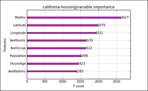
Feature importance should be used with some caution (for GBM and random forest as well). The feature importance metrics are purely based on the tree structure built on the specific model trained with the parameters of that model. This means that if we change the parameters of the model, the importance metrics, and some of the rankings, will change as well. Therefore, it's important to note that for any importance metric, they should not be taken as a generic variable conclusion that generalizes across models.

XGBoost streaming large datasets

In terms of accuracy/performance trade-off, this is simply the best desktop solution. We saw that, with the previous random forest example, we needed to perform subsampling in order to prevent overloading our main memory.

An often-overlooked capability of XGBoost is the method of streaming data through memory. This method parses data through the main memory in a stage-wise fashion to subsequently be parsed into XGBoost model training. This method is a prerequisite to train models on large datasets that are impossible to fit in the main memory. Streaming with XGBoost only works with LIBSVM files, which means that we first have to parse our dataset to the LIBSVM format and import it in the memory cache preserved for XGBoost. Another thing to note is that we use different methods to instantiate XGBoost models. The Scikit-learn-like interface for XGBoost only works on regular NumPy objects. So let's look at how this works.

First, we need to load our dataset in the LIBSVM format and split it into train and test sets before we proceed with preprocessing and training. Parameter tuning with gridsearch is unfortunately not possible with this XGBoost method. If you want to tune parameters, we need to transform the LIBSVM file into a Numpy object, which will dump the data from the memory cache to the main memory. This is unfortunately not scalable, so if you want to perform tuning on large datasets, I would suggest using the reservoir sampling tools we previously introduced and apply tuning to subsamples:

import urllib

from sklearn.datasets import dump_svmlight_file

from sklearn.datasets import load_svmlight_file

trainfile = urllib.URLopener()

trainfile.retrieve("http://www.csie.ntu.edu.tw/~cjlin/libsvmtools/datasets/multiclass/poker.bz2", "pokertrain.bz2")

X,y = load_svmlight_file('pokertrain.bz2')

dump_svmlight_file(X, y,'pokertrain', zero_based=True,query_id=None, multilabel=False)

testfile = urllib.URLopener()

testfile.retrieve("http://www.csie.ntu.edu.tw/~cjlin/libsvmtools/datasets/multiclass/poker.t.bz2", "pokertest.bz2")

X,y = load_svmlight_file('pokertest.bz2')

dump_svmlight_file(X, y,'pokertest', zero_based=True,query_id=None, multilabel=False)

del(X,y)

from sklearn.metrics import classification_report

import numpy as np

import xgboost as xgb

dtrain = xgb.DMatrix('/yourpath/pokertrain#dtrain.cache')

dtest = xgb.DMatrix('/yourpath/pokertest#dtestin.cache')

# For parallelisation it is better to instruct "nthread" to match the exact amount of cpu cores you want #to use.

param = {'max_depth':8,'objective':'multi:softmax','nthread':2,'num_class':10,'verbose':True}

num_round=100

watchlist = [(dtest,'eval'), (dtrain,'train')]

bst = xgb.train(param, dtrain, num_round,watchlist)

print bst

OUTPUT:

[89] eval-merror:0.228659 train-merror:0.016913

[90] eval-merror:0.228599 train-merror:0.015954

[91] eval-merror:0.227671 train-merror:0.015354

[92] eval-merror:0.227777 train-merror:0.014914

[93] eval-merror:0.226247 train-merror:0.013355

[94] eval-merror:0.225397 train-merror:0.012155

[95] eval-merror:0.224070 train-merror:0.011875

[96] eval-merror:0.222421 train-merror:0.010676

[97] eval-merror:0.221881 train-merror:0.010116

[98] eval-merror:0.221922 train-merror:0.009676

[99] eval-merror:0.221733 train-merror:0.009316

We can really experience a great speedup from in-memory XGBoost. We would need a lot more training time if we had used the internal memory version. In this example, we already included the test set as a validation round in the watchlist. However, if we want to predict values on unseen data, we can simply use the same prediction procedure as with any other model in Scikit-learn and XGBoost:

bst.predict(dtest)

OUTPUT:

array([ 0., 0., 1., ..., 0., 0., 1.], dtype=float32)

XGBoost model persistence

In the previous chapter, we covered how to store a GBMmodel to disk to later import and use it for predictions. XGBoost provides the same functionalities. So let's see how we can store and import the model:

import pickle

bst.save_model('xgb.model')

Now you can import the saved model from the directory that you previously specified:

imported_model = xgb.Booster(model_file='xgb.model')

Great, now you can use this model for predictions:

imported_model.predict(dtest)

OUTPUT array([ 9., 9., 9., ..., 1., 1., 1.], dtype=float32)

Out-of-core CART with H2O

Up until now, we have only dealt with desktop solutions for CART models. In Chapter 4, Neural Networks and Deep Learning, we introduced H2O for deep learning out of memory that provided a powerful scalable method. Luckily, H2O also provides tree ensemble methods utilizing its powerful parallel Hadoop ecosystem. As we covered GBM and random forest extensively in previous sections, let's get to it right away. For this exercise, we will use the spam dataset that we used before.

Random forest and gridsearch on H2O

Let's implement a random forest with gridsearch hyperparameter optimization. In this section, we first load the spam dataset from the URL source:

import pandas as pd

import numpy as np

import os

import xlrd

import urllib

import h2o

#set your path here

os.chdir('/yourpath/')

url = 'https://archive.ics.uci.edu/ml/machine-learning-databases/spambase/spambase.data'

filename='spamdata.data'

urllib.urlretrieve(url, filename)

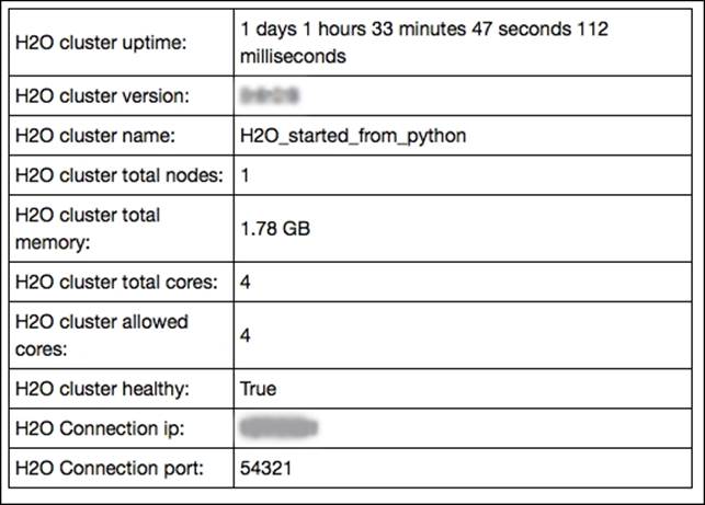
Now that we have loaded the data, we can initialize the H2O session:

h2o.init(max_mem_size_GB = 2)

OUTPUT:

Here, we preprocess the data where we split the data into train, validation, and test sets. We do this with an H2O function (.split_frame). Also note the important step where we convert the target vector C58 to a factor variable:

spamdata = h2o.import_file(os.path.realpath("/yourpath/"))

spamdata['C58']=spamdata['C58'].asfactor()

train, valid, test= spamdata.split_frame([0.6,.2], seed=1234)

spam_X = spamdata.col_names[:-1]

spam_Y = spamdata.col_names[-1]

In this part, we will set up the parameters that we will optimize with gridsearch. First of all, we set the number of trees in the model to a single value of 300. The parameters that are iterated with gridsearch are as follows:

· max_depth: The maximum depth of the tree

· balance_classes: Each iteration uses balanced classes for the target outcome

· sample_rate: This is the fraction of the rows that are sampled for each iteration

Now let's pass these parameters into a Python list to be used in our H2O gridsearch model:

hyper_parameters={'ntrees':[300], 'max_depth':[3,6,10,12,50],'balance_classes':['True','False'],'sample_rate':[.5,.6,.8,.9]}

grid_search = H2OGridSearch(H2ORandomForestEstimator, hyper_params=hyper_parameters)

grid_search.train(x=spam_X, y=spam_Y,training_frame=train)

print 'this is the optimum solution for hyper parameters search %s' % grid_search.show()

OUTPUT:

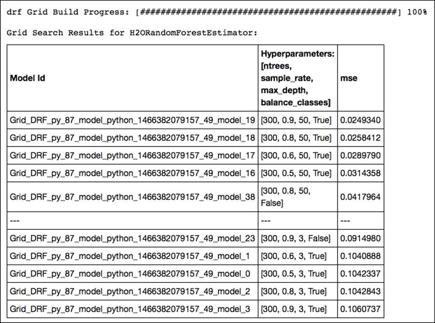
Of all the possible combinations, the model with a row sample rate of .9, a tree depth of 50, and balanced classes yields the highest accuracy. Now let's train a new random forest model with optimal parameters resulting from our gridsearch and predict the outcome on the test set:

final = H2ORandomForestEstimator(ntrees=300, max_depth=50,balance_classes=True,sample_rate=.9)

final.train(x=spam_X, y=spam_Y,training_frame=train)

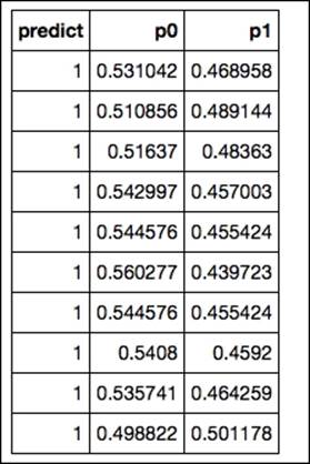
print final.predict(test)

The final output of the predictions in H2O results in an array with the first column containing the actual predicted classes and columns containing the class probabilities of each target label:

OUTPUT:

Stochastic gradient boosting and gridsearch on H2O

We have seen in previous examples that most of the time, a well-tuned GBM model outperforms random forest. So now let's perform a GBM with gridsearch in H2O and see if we can improve our score. For this session, we introduce the same random subsampling method that we used for the random forest model in H2O (sample_rate). Based on Jerome Friedman's article (https://statweb.stanford.edu/~jhf/ftp/stobst.pdf) from 1999, a method named stochastic gradient boosting was introduced. This stochasticity added to the model utilizes random subsampling without replacement from the data at each tree iteration that is considered to prevent overfitting and increase overall accuracy. In this example, we take this idea of stochasticity further by introducing random subsampling based on the features at each iteration.

This method of randomly subsampling features is also referred to as the random subspace method, which we have already seen in the Random forest and extremely randomized forest section of this chapter. We achieve this with the col_sample_rate parameter. So to summarize, in this GBM model, we are going to perform gridsearch optimization on the following parameters:

· max_depth: Maximum tree depth

· sample_rate: Fraction of the rows used at each iteration

· col_sample_rate: Fraction of the features used at each iteration

We use exactly the same spam dataset as the previous section so we can get right down to it:

hyper_parameters={'ntrees':[300],'max_depth':[12,30,50],'sample_rate':[.5,.7,1],'col_sample_rate':[.9,1],

'learn_rate':[.01,.1,.3],}

grid_search = H2OGridSearch(H2OGradientBoostingEstimator, hyper_params=hyper_parameters)

grid_search.train(x=spam_X, y=spam_Y, training_frame=train)

print 'this is the optimum solution for hyper parameters search %s' % grid_search.show()

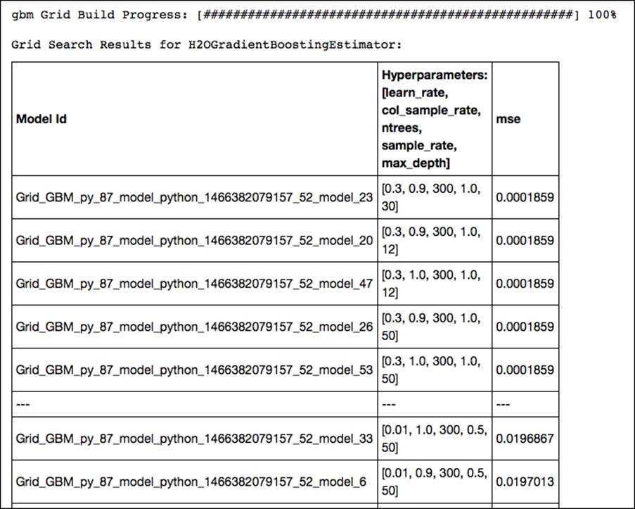
gbm Grid Build Progress: [##################################################] 100%

The upper part of our gridsearch output shows that we should use an exceptionally high learning rate of .3, a column sample rate of .9, and a maximum tree depth of 30. Random subsampling based on rows didn't increase performance, but subsampling based on features with a fraction of .9 was quite effective in this case. Now let's train a new GBM model with the optimal parameters resulting from our gridsearch optimization and predict the outcome on the test set:

spam_gbm2 = H2OGradientBoostingEstimator(

ntrees=300,

learn_rate=0.3,

max_depth=30,

sample_rate=1,

col_sample_rate=0.9,

score_each_iteration=True,

seed=2000000

)

spam_gbm2.train(spam_X, spam_Y, training_frame=train, validation_frame=valid)

confusion_matrix = spam_gbm2.confusion_matrix(metrics="accuracy")

print confusion_matrix

OUTPUT:

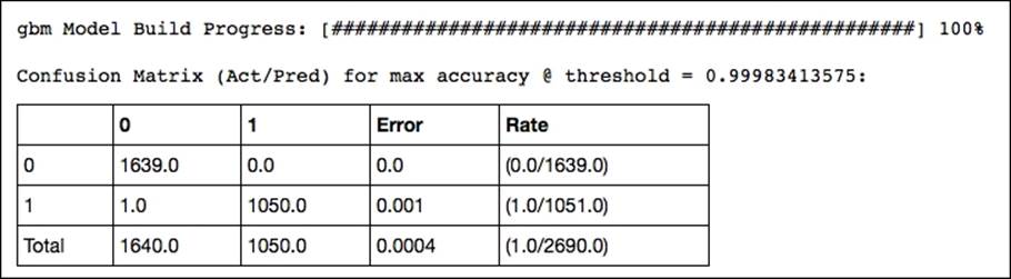
This delivers interesting diagnostics of the model's performance such as accuracy, rmse, logloss, and AUC. However, its output is too large to include here. Look at the output of your IPython notebook for the complete output.

You can utilize this with the following:

print spam_gbm2.score_history()

Of course, the final predictions can be achieved as follows:

print spam_gbm2.predict(test)

Great, we have been able to improve the accuracy of our model close to 100%. As you can see, in H2O, you might be less flexible in terms of modeling and munging your data, but the speed of processing and accuracy that can be achieved is unrivaled. To round off this session, you can do the following:

h2o.shutdown(prompt=False)

Summary

We saw that CART methods trained with ensemble routines are powerful when it comes to predictive accuracy. However, they can be computationally expensive and we have covered some techniques in speeding them up in sklearn's applications. We noticed that using extreme randomized forests tuned with randomized search could speed up by tenfold when used properly. For GBM, however, there is no parallelization implemented in sklearn, and this is exactly where XGBoost comes in.

XGBoost comes with an effective parallelized boosting algorithm speeding up the algorithm nicely. When we use larger files (>100k training examples), there is an out-of-core method that makes sure we don't overload our main memory while training models.

The biggest gains in speed and memory can be found with H2O; we saw powerful tuning capabilities together with an impressive training speed.