Large Scale Machine Learning with Python (2016)

Chapter 7. Unsupervised Learning at Scale

In the previous chapters, the focus of the problem was on predicting a variable, which could have been a number, class, or category. In this chapter, we will change the approach and try to create new features and variables at scale, hopefully better for our prediction purposes than the ones already included in the observation matrix. We will first introduce the unsupervised methods and illustrate three of them, which are able to scale to big data:

· Principal Component Analysis (PCA), an effective way to reduce the number of features

· K-means, a scalable algorithm for clustering

· Latent Dirichlet Allocation (LDA), a very effective algorithm able to extract topics from a series of text documents

Unsupervised methods

Unsupervised learning is a branch of machine learning whose algorithms reveal inferences from data without an explicit label (unlabeled data). The goal of such techniques is to extract hidden patterns and group similar data.

In these algorithms, the unknown parameters of interests of each observation (the group membership and topic composition, for instance) are often modeled as latent variables (or a series of hidden variables), hidden in the system of observed variables that cannot be observed directly, but only deduced from the past and present outputs of the system. Typically, the output of the system contains noise, which makes this operation harder.

In common problems, unsupervised methods are used in two main situations:

· With labeled datasets to extract additional features to be processed by the classifier/regressor down to the processing chain. Enhanced by additional features, they may perform better.

· With labeled or unlabeled datasets to extract some information about the structure of the data. This class of algorithms is commonly used during the Exploratory Data Analysis (EDA) phase of the modeling.

First of all, before starting with our illustration, let's import the modules that will be necessary along the chapter in our notebook:

In : import matplotlib

import numpy as np

import pandas as pd

import matplotlib.pyplot as plt

from matplotlib import pylab

%matplotlib inline

import matplotlib.cm as cm

import copy

import tempfile

import os

Feature decomposition – PCA

PCA is an algorithm commonly used to decompose the dimensions of an input signal and keep just the principal ones. From a mathematical perspective, PCA performs an orthogonal transformation of the observation matrix, outputting a set of linear uncorrelated variables, named principal components. The output variables form a basis set, where each component is orthonormal to the others. Also, it's possible to rank the output components (in order to use just the principal ones) as the first component is the one containing the largest possible variance of the input dataset, the second is orthogonal to the first (by definition) and contains the largest possible variance of the residual signal, and the third is orthogonal to the first two and it's built on the residual variance, and so on.

A generic transformation with PCA can be expressed as a projection to a space. If just the principal components are taken from the transformation basis, the output space will have a smaller dimensionality than the input one. Mathematically, it can be expressed as follows:

Here, X is a generic point of the training set of dimension N, T is the transformation matrix coming from PCA, and is the output vector. Note that the symbol indicates a dot product in this matrix equation. From a practical perspective, also note that all the features of X must be zero-centered before doing this operation.

Let's now start with a practical example; later, we will explain math PCA in depth. In this example, we will create a dummy dataset composed of two blobs of points—one cantered in (-5, 0) and the other one in (5, 5).Let's use PCA to transform the dataset and plot the output compared to the input. In this simple example, we will use all the features, that is, we will not perform feature reduction:

In:from sklearn.datasets.samples_generator import make_blobs

from sklearn.decomposition import PCA

X, y = make_blobs(n_samples=1000, random_state=101, \

centers=[[-5, 0], [5, 5]])

pca = PCA(n_components=2)

X_pca = pca.fit_transform(X)

pca_comp = pca.components_.T

test_point = np.matrix([5, -2])

test_point_pca = pca.transform(test_point)

plt.subplot(1, 2, 1)

plt.scatter(X[:, 0], X[:, 1], c=y, edgecolors='none')

plt.quiver(0, 0, pca_comp[:,0], pca_comp[:,1], width=0.02, \

scale=5, color='orange')

plt.plot(test_point[0, 0], test_point[0, 1], 'o')

plt.title('Input dataset')

plt.subplot(1, 2, 2)

plt.scatter(X_pca[:, 0], X_pca[:, 1], c=y, edgecolors='none')

plt.plot(test_point_pca[0, 0], test_point_pca[0, 1], 'o')

plt.title('After "lossless" PCA')

plt.show()

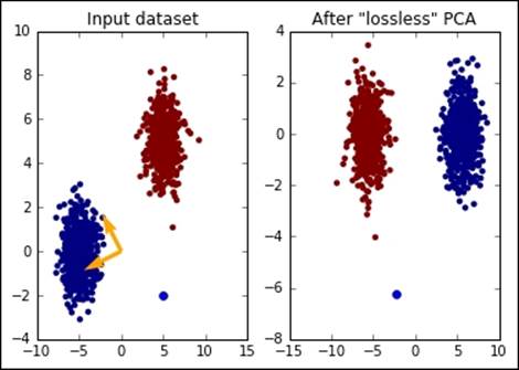
As you can see, the output is more organized than the original features' space and, if the next task is a classification, it would require just one feature of the dataset, saving almost 50% of the space and computation needed. In the image, you can clearly see the core of PCA: it's just a projection of the input dataset to the transformation basis drawn in the image on the left in orange. Are you unsure about this? Let's test it:

In:print "The blue point is in", test_point[0, :]

print "After the transformation is in", test_point_pca[0, :]

print "Since (X-MEAN) * PCA_MATRIX = ", np.dot(test_point - \

pca.mean_, pca_comp)

Out:The blue point is in [[ 5 -2]]

After the transformation is in [-2.34969911 -6.2575445 ]

Since (X-MEAN) * PCA_MATRIX = [[-2.34969911 -6.2575445 ]

Now, let's dig into the core problem: how is it possible to generate T from the training set? It should contain orthonormal vectors, and the vectors should be ranked according to the quantity of variance (that is, the energy or information carried by the observation matrix) that they can explain. Many solutions have been implemented, but the most common implementation is based on Singular Value Decomposition (SVD).

SVD is a technique that decomposes any matrix M into three matrixes with special properties and whose multiplication gives back M again:

Specifically, given M, a matrix of m rows and n columns, the resulting elements of the equivalence are as follows:

· U is a matrix m x m (square matrix), it's unitary, and its columns form an orthonormal basis. Also, they're named left singular vectors, or input singular vectors, and they're the eigenvectors of the matrix product .

· is a matrix m x n, which has only non-zero elements on its diagonal. These values are named singular values, are all non-negative, and are the eigenvalues of both and .

· W is a unitary matrix n x n (square matrix), its columns form an orthonormal basis, and they're named right (or output) singular vectors. Also, they are the eigenvectors of the matrix product .

Why is this needed? The solution is pretty easy: the goal of PCA is to try and estimate the directions where the variance of the input dataset is larger. For this, we first need to remove the mean from each feature and then operate on the covariance matrix .

Given that, by decomposing the matrix X with SVD, we have the columns of the matrix W that are the principal components of the covariance (that is, the matrix T we are looking for), the diagonal of that contains the variance explained by the principal components, and the columns of U the principal components. Here's why PCA is always done with SVD.

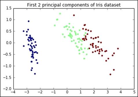
Let's see it now on a real example. Let's test it on the Iris dataset, extracting the first two principal components (that is, passing from a dataset composed by four features to one composed by two):

In:from sklearn import datasets

iris = datasets.load_iris()

X = iris.data

y = iris.target

print "Iris dataset contains", X.shape[1], "features"

pca = PCA(n_components=2)

X_pca = pca.fit_transform(X)

print "After PCA, it contains", X_pca.shape[1], "features"

print "The variance is [% of original]:", \

sum(pca.explained_variance_ratio_)

plt.scatter(X_pca[:, 0], X_pca[:, 1], c=y, edgecolors='none')

plt.title('First 2 principal components of Iris dataset')

plt.show()

Out:Iris dataset contains 4 features

After PCA, it contains 2 features

The variance is [% of original]: 0.977631775025

This is the analysis of the outputs of the process:

· The explained variance is almost 98% of the original variance from the input. The number of features has been halved, but only 2% of the information is not in the output, hopefully just noise.

· From a visual inspection, it seems that the different classes, composing the Iris dataset, are separated from each other. This means that a classifier working on such a reduced set will have comparable performance in terms of accuracy, but will be faster to train and run prediction.

As a proof of the second point, let's now try to train and test two classifiers, one using the original dataset and another using the reduced set, and print their accuracy:

In:from sklearn.linear_model import SGDClassifier

from sklearn.cross_validation import train_test_split

from sklearn.metrics import accuracy_score

def test_classification_accuracy(X_in, y_in):

X_train, X_test, y_train, y_test = \

train_test_split(X_in, y_in, random_state=101, \

train_size=0.50)

clf = SGDClassifier('log', random_state=101)

clf.fit(X_train, y_train)

return accuracy_score(y_test, clf.predict(X_test))

print "SGDClassifier accuracy on Iris set:", \

test_classification_accuracy(X, y)

print "SGDClassifier accuracy on Iris set after PCA (2 components):", \

test_classification_accuracy(X_pca, y)

Out:SGDClassifier accuracy on Iris set: 0.586666666667

SGDClassifier accuracy on Iris set after PCA (2 components): 0.72

As you can see, this technique not only reduces the complexity and space of the learner down in the chain, but also helps achieve generalization (exactly as a Ridge or Lasso regularization).

Now, if you are unsure how many components should be in the output, typically as a rule of thumb, choose the minimum number that is able to explain at least 90% (or 95%) of the input variance. Empirically, such a choice usually ensures that only the noise is cut off.

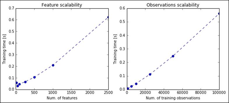
So far, everything seems perfect: we found a great solution to reduce the number of features, building some with very high predictive power, and we also have a rule of thumb to guess the right number of them. Let's now check how scalable this solution is: we're investigating how it scales when the number of observations and features increases. The first thing to note is that the SVD algorithm, the core piece of PCA, is not stochastic; therefore, it needs the whole matrix in order to be able to extract its principal components. Now, let's see how scalable PCA is in practice on some synthetic datasets with an increasing number of features and observations. We will perform a full (lossless) decomposition (the argument while instantiating the object PCA is None), as asking for a lower number of features doesn't impact the performance (it's just a matter of slicing the output matrixes of SVD).

In the following code, we first create matrixes with 10,000 points and 20, 50, 100, 250, 1,000, and 2,500 features to be processed by PCA. Then, we create matrixes with 100 features and 1, 5, 10, 25, 50, and 100 thousand observations to be processed with PCA:

In:import time

def check_scalability(test_pca):

pylab.rcParams['figure.figsize'] = (10, 4)

# FEATURES

n_points = 10000

n_features = [20, 50, 100, 250, 500, 1000, 2500]

time_results = []

for n_feature in n_features:

X, _ = make_blobs(n_points, n_features=n_feature, \

random_state=101)

pca = copy.deepcopy(test_pca)

tik = time.time()

pca.fit(X)

time_results.append(time.time()-tik)

plt.subplot(1, 2, 1)

plt.plot(n_features, time_results, 'o--')

plt.title('Feature scalability')

plt.xlabel('Num. of features')

plt.ylabel('Training time [s]')

# OBSERVATIONS

n_features = 100

n_observations = [1000, 5000, 10000, 25000, 50000, 100000]

time_results = []

for n_points in n_observations:

X, _ = make_blobs(n_points, n_features=n_features, \

random_state=101)

pca = copy.deepcopy(test_pca)

tik = time.time()

pca.fit(X)

time_results.append(time.time()-tik)

plt.subplot(1, 2, 2)

plt.plot(n_observations, time_results, 'o--')

plt.title('Observations scalability')

plt.xlabel('Num. of training observations')

plt.ylabel('Training time [s]')

plt.show()

check_scalability(PCA(None))

Out:

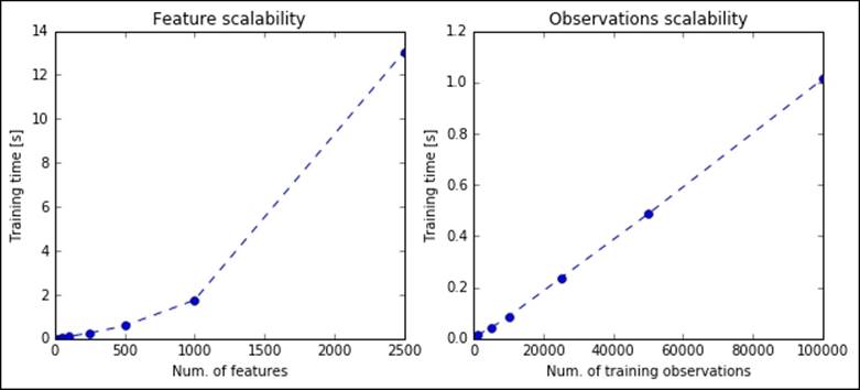
As you can clearly see, PCA based on SVD is not scalable: if the number of features increases linearly, the time needed to train the algorithm increases exponentially. Also, the time needed to process a matrix with a few hundred observations becomes too high and (not shown in the image) the memory consumption makes the problem unfeasible for a domestic computer (with 16 or fewer GB of RAM). It seems clear that a PCA based on SVD is not the solution for big data; fortunately, in recent years, many workarounds have been introduced. In the following sections, you'll find a short introduction for each of them.

Randomized PCA

The correct name of this technique should be PCA based on randomized SVD, but it has become popular with the name Randomized PCA. The core idea behind the randomization is the redundancy of all the principal components; in fact, if the goal of the method is dimension reduction, one should expect that only a few vectors are needed in the output (the K principal ones). By focusing on the problem of finding the best K principal vectors, the algorithm scales more. Note that in this algorithm, K—the number of principal components to be outputted—is a key parameter: set it too large and the performance won't be better than PCA; set it too low and the variance explained with the resulting vectors will be too low.

As in PCA, we want to find an approximation of the matrix containing observations X, such that ; we also want the matrix Q with K orthonormal columns (they will be called principal components). With SVD, we can now compute the decomposition of thesmall matrix . As we proved, it won't take a long time. As , by taking , we now have a truncated approximation of X based on a low rank SVD, .

Mathematically, it seems perfect, but there are still two missing points: what role does the randomization have? How to get the matrix Q? Both questions are answered here: a Gaussian random matrix is extracted, , and it's computed Y as . Then, Y is QR-decomposed, creating , and here is Q, the matrix of K orthonormal columns that we are looking for.

The math underneath this decomposition is pretty heavy, and fortunately everything has been implemented in Scikit-learn, so you don't need to figure out how to deal with Gaussian random variables and so on. Let's initially see how bad it performs when a full (lossless) decomposition is computed with randomized PCA:

In:from sklearn.decomposition import RandomizedPCA

check_scalability(RandomizedPCA(None))

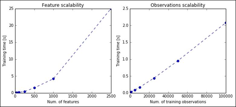
Performances are worse than the classic PCA; in fact, this transformation works very well when a reduced set of components is asked. Let's now see the performance when K=20:

In:check_scalability(RandomizedPCA(20))

As expected, the computations are very quick; in less than a second, the algorithm is able to perform the most complex factorizations.

Checking the results and the algorithm, we still notice something odd: the training dataset, X, must all fit in-memory in order to be decomposed, even in the case of the randomized PCA. Does an online version of PCA exist that is able to incrementally fit the principal vectors without having the whole dataset in-memory? Yes, there is—incremental PCA.

Incremental PCA

Incremental PCA, or mini-batch PCA, is the online version of Principal Component Analysis. The core of the algorithm is very simple: the batch of data is initially split into mini-batches with the same number of observations. (The only limitation is that the number of observations per mini-batch should be greater than the number of features.) Then, the first mini-batch is centered (the mean is removed) and its SVD decomposition is performed, storing the principal components. Then, when the next mini-batch enters the process, it's first centered and then stacked with the principal components extracted from the previous mini-batch (they're inserted as additional observations). Now, another SVD is performed and the principal components are overwritten with the new ones. The process goes till the last mini-batch: for each of them, first there is the centering, then the stacking, and finally the SVD. Doing so, instead of a big SVD, we're performing as many small SVD as the number of mini-batches.

As you can understand, this technique doesn't outperform randomized PCA, but its goal is to offer a solution (or the only solution) when PCA is needed on a dataset that doesn't fit in-memory. Incremental PCA doesn't run to win a speed challenge, but to limit memory consumption; the memory usage is constant throughout the training and can be tuned by setting the mini-batch size. As a rule of thumb, the memory footprint is approximately the same order of magnitude as the square of the size of the mini-batch.

As a code example, let's now check how incremental PCA is able to cope with a large dataset, which is, in our exemplification, composed of 10 million observations and 100 features. None of the previous algorithms are able to do so, unless you want to crash your computer (or witness an enormous amount of swap between memory and the storage disk). With incremental PCA, such a task turns into a piece of cake and, all things considered, the process is not all that slow (Note that we're doing a complete lossless decomposition with a stable amount of memory consumed):

In:from sklearn.decomposition import IncrementalPCA

X, _ = make_blobs(100000, n_features=100, random_state=101)

pca = IncrementalPCA(None, batch_size=1000)

tik = time.time()

for i in range(100):

pca.partial_fit(X)

print "PCA on 10M points run with constant memory usage in ", \

time.time() - tik, "seconds"

Out:PCA on 10M points run with constant memory usage in 155.642718077 seconds

Sparse PCA

Sparse PCA operates in a different way than the previous algorithms; instead of operating a feature reduction using an SVD applied on the covariance matrix (after being centered), it operates a feature selection-like operation of that matrix, finding the set of sparse components that best reconstruct the data. As in Lasso regularization, the amount of sparseness is controllable by a penalty (or constraint) on the coefficients.

With respect to PCA, sparse PCA doesn't guarantee that the resulting components will be orthogonal, but the result is more interpretable as principal vectors are actually a portion of the input dataset. Moreover, it's scalable in terms of the number of features: if PCA and its scalable versions are stuck when the number of features is getting larger (let's say, more than 1,000), sparse PCA is still an optimal solution in terms of speed thanks to the internal method to solve the Lasso problem, typically based on Lars or Coordinate Descent. (Remember that Lasso tries to minimize the L1 norm of the coefficients.) Moreover, it's great when the number of features is greater than the number of observations as, for example, some image datasets.

Let's now see how it works on a 25,000 observations dataset with 10,000 features. For this example, we're using the mini-batch version of the SparsePCA algorithm that ensures constant memory usage and is able to cope with massive datasets, eventually larger than the available memory (note that the batch version is named SparsePCA but doesn't support the online training):

In:from sklearn.decomposition import MiniBatchSparsePCA

X, _ = make_blobs(25000, n_features=10000, random_state=101)

tik = time.time()

pca = MiniBatchSparsePCA(20, method='cd', random_state=101, \

n_iter=1000)

pca.fit(X)

print "SparsePCA on matrix", X.shape, "done in ", time.time() - \

tik, "seconds"

Out:

SparsePCA on matrix (25000, 10000) done in 41.7692570686 seconds

In about 40 seconds, SparsePCA is able to produce a solution using a constant amount of memory.

PCA with H2O

We can also use the PCA implementation provided by H2O. (We've already seen H2O in the previous chapter and mentioned it along the book.)

With H2O, we first need to turn on the server with the init method. Then, we dump the dataset on a file (precisely, a CSV file) and finally run the PCA analysis. As the last step, we shut down the server.

We're trying this implementation on some of the biggest datasets seen so far—the one with 100K observations and 100 features and the one with 10K observations and 2,500 features:

In: import h2o

from h2o.transforms.decomposition import H2OPCA

h2o.init(max_mem_size_GB=4)

def testH2O_pca(nrows, ncols, k=20):

temp_file = tempfile.NamedTemporaryFile().name

X, _ = make_blobs(nrows, n_features=ncols, random_state=101)

np.savetxt(temp_file, np.c_[X], delimiter=",")

del X

pca = H2OPCA(k=k, transform="NONE", pca_method="Power")

tik = time.time()

pca.train(x=range(100), \

training_frame=h2o.import_file(temp_file))

print "H2OPCA on matrix ", (nrows, ncols), \

" done in ", time.time() - tik, "seconds"

os.remove(temp_file)

testH2O_pca(100000, 100)

testH2O_pca(10000, 2500)

h2o.shutdown(prompt=False)

Out:[...]

H2OPCA on matrix (100000, 100) done in 12.9560530186 seconds

[...]

H2OPCA on matrix (10000, 2500) done in 10.1429388523 seconds

As you can see, in both cases, H2O indeed performs very fast and is well-comparable (if not outperforming) to Scikit-learn.

Clustering – K-means

K-means is an unsupervised algorithm that creates K disjoint clusters of points with equal variance, minimizing the distortion (also named inertia).

Given only one parameter K, representing the number of clusters to be created, the K-means algorithm creates K sets of points S₁, S₂, …, S_K, each of them represented by its centroid: C₁, C₂, …, C_K. The generic centroid, C_i, is simply the mean of the samples of the points associated to the cluster Si in order to minimize the intra-cluster distance. The outputs of the system are as follows:

1. The composition of the clusters S₁, S₂, …, S_K, that is, the set of points composing the training set that are associated to the cluster number 1, 2, …, K.

2. The centroids of each cluster, C₁, C₂, …, C_K. Centroids can be used for future associations.

3. The distortion introduced by the clustering, computed as follows:

This equation denotes the optimization intrinsically done in the K-means algorithm: the centroids are chosen to minimize the intra-cluster distortion, that is, the sum of Euclidean norms of the distances between each input point and the centroid of the cluster to which the point is associated to. In other words, the algorithm tries to fit the best vectorial quantization.

The training phase of the K-means algorithm is also called Lloyd's algorithm, named after Stuart Lloyd, who first proposed the algorithm. It's an iterative algorithm composed of two phases iterated over and over till convergence (the distortion reaches a minimum). It's a variant of the generalized expectation-maximization (EM) algorithm as the first step creates a function for the expectation (E) of a score, and the maximization (M) step computes the parameters that maximize the score. (Note that in this formulation, we try to achieve the opposite, that is, the minimization of the distortion.) Here's its formulation:

· The expectation step: In this step, the points in the training set are assigned to the closest centroid:

This step is also named assignment or vectorial quantization.

· The maximization step: The centroid of each cluster is moved to the middle of the cluster by averaging the points composing it:

This step is also named update step.

These two steps are performed till convergence (points are stable in their cluster), or till the algorithm reaches a preset number of iterations. Note that, per composition, the distortion cannot increase throughout the training phase (unlike Stochastic Gradient Descent-based methods); therefore, in this algorithm, the more iterations, the better the result.

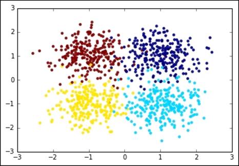
Let's now see how it looks like on a dummy two-dimensional dataset. We first create a set of 1,000 points concentrated in four locations symmetric with respect to the origin. Each cluster, per construction, has the same variance:

In:import matplotlib

import numpy as np

import pandas as pd

import matplotlib.pyplot as plt

%matplotlib inline

In:from sklearn.datasets.samples_generator import make_blobs

centers = [[1, 1], [1, -1], [-1, -1], [-1, 1]]

X, y = make_blobs(n_samples=1000, centers=centers,

cluster_std=0.5, random_state=101)

Let's now plot the dataset. To make things easier, we will color the clusters with different colors:

In:plt.scatter(X[:,0], X[:,1], c=y, edgecolors='none', alpha=0.9)

plt.show()

Let's now run K-means and inspect what's going on at each iteration. For this, we stop the iteration to 1, 2, 3, and 4 iterations and plot the points with their associated cluster (color-coded) as well as the centroid, distortion (in the title), and decision boundaries (also named Voronoi cells). The initial choice of the centroids is at random, that is, four training points are elected centroids in the first iteration during the expectation phase of the training:

In:pylab.rcParams['figure.figsize'] = (10.0, 8.0)

from sklearn.cluster import KMeans

for n_iter in range(1, 5):

cls = KMeans(n_clusters=4, max_iter=n_iter, n_init=1,

init='random', random_state=101)

cls.fit(X)

# Plot the voronoi cells

plt.subplot(2, 2, n_iter)

h=0.02

xx, yy = np.meshgrid(np.arange(-3, 3, h), np.arange(-3, 3, h))

Z = cls.predict(np.c_[xx.ravel(), \

yy.ravel()]).reshape(xx.shape)

plt.imshow(Z, interpolation='nearest', cmap=plt.cm.Accent, \

extent=(xx.min(), xx.max(), yy.min(), yy.max()), \

aspect='auto', origin='lower')

plt.scatter(X[:,0], X[:,1], c=cls.labels_, \

edgecolors='none', alpha=0.7)

plt.scatter(cls.cluster_centers_[:,0], \

cls.cluster_centers_[:,1], \

marker='x', color='r', s=100, linewidths=4)

plt.title("iter=%s, distortion=%s" %(n_iter, \

int(cls.inertia_)))

plt.show()

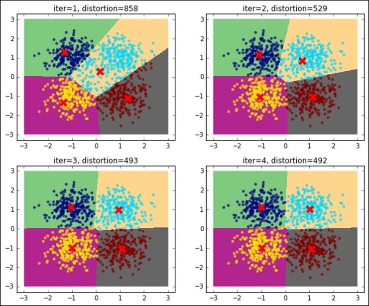
As you can see, the distortion is getting lower and lower as the number of iterations increases. For this dummy dataset, it seems that using a few iterations (five iterations), we've reached the convergence.

Initialization methods

Finding the global minimum of the distortion in K-means is a NP-hard problem; moreover, exactly as with Stochastic Gradient Descent, this method is prone to converge to local minima especially if the number of dimensions is high. In order to avoid such behavior and limit the maximum number of iterations, you can use the following countermeasures:

· Run the algorithm multiple times using different initial conditions. In Scikit-learn, the KMeans class has the n_init parameter that controls how many times the K-means algorithm will be run with different centroid seeds. At the end, the model that ensures the lower distortion is selected. If multiple cores are available, this process can be run in parallel by setting the n_jobs parameter to the number of desired jobs to spin off. Note that the memory consumption is linearly dependent on the number of parallel jobs.

· Prefer the k-means++ initialization (the KMeans class is the default) to the random choice of training points. K-means++ initialization selects points that are far among each other; this should ensure that the centroids are able to form clusters in uniform subspaces of the space. It's also proved that this fact ensures that it's more likely to find the best solution.

K-means assumptions

K-means relies on the assumptions that each cluster has a (hyper-) spherical shape, that is, it doesn't have an elongated shape (like an arrow), all the clusters have the same variance internally, and their size is comparable (or they are very far away).

All of these hypotheses can be guaranteed with a strong feature preprocessing step; PCA, KernelPCA, feature normalization, and sampling can be a good start.

Let's now see what happens when the assumptions behind K-means are not met:

In:pylab.rcParams['figure.figsize'] = (5.0, 10.0)

from sklearn.datasets import make_moons

# Oblong/elongated sets

X, _ = make_moons(n_samples=1000, noise=0.1, random_state=101)

cls = KMeans(n_clusters=2, random_state=101)

y_pred = cls.fit_predict(X)

plt.subplot(3, 1, 1)

plt.scatter(X[:, 0], X[:, 1], c=y_pred, edgecolors='none')

plt.scatter(cls.cluster_centers_[:,0], cls.cluster_centers_[:,1],

marker='x', color='r', s=100, linewidths=4)

plt.title("Elongated clusters")

# Different variance between clusters

centers = [[-1, -1], [0, 0], [1, 1]]

X, _ = make_blobs(n_samples=1000, cluster_std=[0.1, 0.4, 0.1],

centers=centers, random_state=101)

cls = KMeans(n_clusters=3, random_state=101)

y_pred = cls.fit_predict(X)

plt.subplot(3, 1, 2)

plt.scatter(X[:, 0], X[:, 1], c=y_pred, edgecolors='none')

plt.scatter(cls.cluster_centers_[:,0], cls.cluster_centers_[:,1],

marker='x', color='r', s=100, linewidths=4)

plt.title("Unequal Variance between clusters")

# Unevenly sized blobs

centers = [[-1, -1], [1, 1]]

centers.extend([[0,0]]*20)

X, _ = make_blobs(n_samples=1000, centers=centers,

cluster_std=0.28, random_state=101)

cls = KMeans(n_clusters=3, random_state=101)

y_pred = cls.fit_predict(X)

plt.subplot(3, 1, 3)

plt.scatter(X[:, 0], X[:, 1], c=y_pred, edgecolors='none')

plt.scatter(cls.cluster_centers_[:,0], cls.cluster_centers_[:,1],

marker='x', color='r', s=100, linewidths=4)

plt.title("Unevenly Sized Blobs")

plt.show()

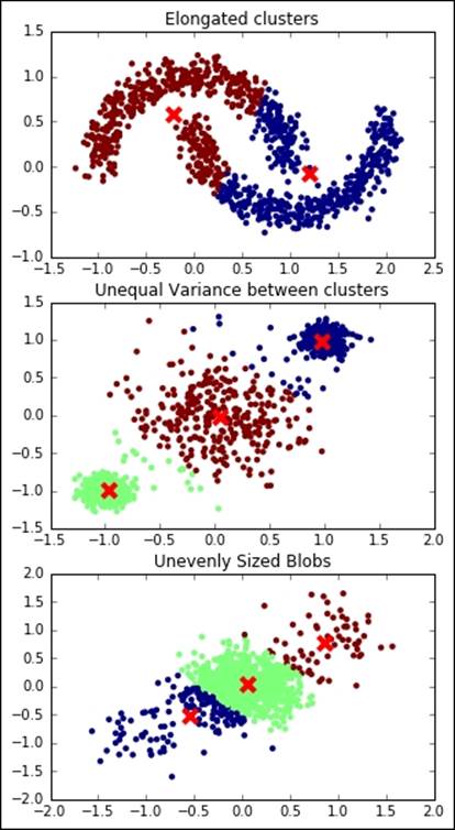
In all the preceding examples, the clustering operation is not perfect, outputting a wrong and unstable result.

So far, we've assumed to know exactly which is the exact K, the number of clusters that we're expecting to use in the clustering operation. Actually, in real-world problems, this is not always true. We often use an unsupervised learning method to discover the underlying structure of the data, including the number of clusters composing the dataset. Let's see what happens when we try to run K-means with a wrong K on a simple dummy dataset; we will try both a lower K and a higher one:

In:pylab.rcParams['figure.figsize'] = (10.0, 4.0)

X, _ = make_blobs(n_samples=1000, centers=3, random_state=101)

for K in [2, 3, 4]:

cls = KMeans(n_clusters=K, random_state=101)

y_pred = cls.fit_predict(X)

plt.subplot(1, 3, K-1)

plt.title("K-means, K=%s" % K)

plt.scatter(X[:, 0], X[:, 1], c=y_pred, edgecolors='none')

plt.scatter(cls.cluster_centers_[:,0], cls.cluster_centers_[:,1],

marker='x', color='r', s=100, linewidths=4)

plt.show()

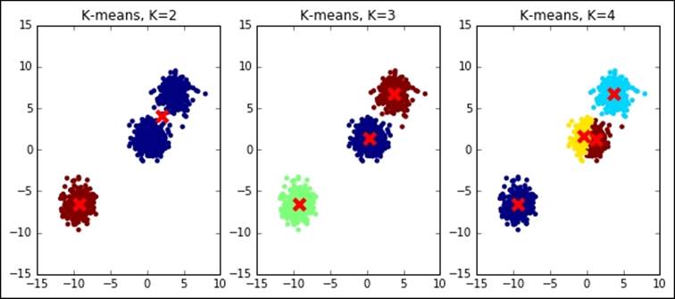
As you can see, the results are massively wrong in case the right K is not guessed, even for this simple dummy dataset. In the next section, we will explain some tricks to best select the K.

Selection of the best K

There are several methods to detect the best K if the assumptions behind K-means are met. Some of them are based on cross-validation and metrics on the output; they can be used on all clustering methods, but only when a ground truth is available (they're named supervised metrics). Some others are based on intrinsic parameters of the clustering algorithm and can be used independently by the presence or absence of the ground truth (also named unsupervised metrics). Unfortunately, none of them ensures 100% accuracy to find the correct result.

Supervised metrics require a ground truth (containing the true associations in sets) and they're usually combined with a gridsearch analysis to understand the best K. Some of these metrics are derived from equivalent classification ones, but they allow having a different number of unordered sets as predicted labels. The first one that we're going to see is named homogeneity; as you can expect, it gives a measure of how many of the predicted clusters contain just points of one class. It's a measure based on entropy, and it's the cluster equivalent of the precision in classification. It's a measure bound between 0 (worst) and 1 (best); its mathematical formulation is as follows:

Here, H(C|K) is the conditional entropy of the class distribution given the proposed clustering assignment, and H(C) is the entropy of the classes. H(C|K) is maximal and equals H(C) when the clustering provides no new information; it is zero when each cluster contains only a member of a single class.

Connected to it, as in precision and recall for classification, there is the completeness score: it gives a measure about how much all members of a class are assigned to the same cluster. Even this one is bound between 0 (worst) and 1 (best), and its mathematical formulation is deeply based on entropy:

Here, H(K|C) is the conditional entropy of the proposed cluster distribution given the class, and H(K) is the entropy of the clusters.

Finally, equivalent to the f1 score for the classification task, the V-measure is the harmonic mean of homogeneity and completeness:

Let's get back to the first dataset (four symmetric noisy clusters), and try to see how these scores operate and whether they are able to highlight the best K to use:

In:pylab.rcParams['figure.figsize'] = (6.0, 4.0)

from sklearn.metrics import homogeneity_completeness_v_measure

centers = [[1, 1], [1, -1], [-1, -1], [-1, 1]]

X, y = make_blobs(n_samples=1000, centers=centers,

cluster_std=0.5, random_state=101)

Ks = range(2, 10)

HCVs = []

for K in Ks:

y_pred = KMeans(n_clusters=K, random_state=101).fit_predict(X)

HCVs.append(homogeneity_completeness_v_measure(y, y_pred))

plt.plot(Ks, [el[0] for el in HCVs], 'r', label='Homogeneity')

plt.plot(Ks, [el[1] for el in HCVs], 'g', label='Completeness')

plt.plot(Ks, [el[2] for el in HCVs], 'b', label='V measure')

plt.ylim([0, 1])

plt.legend(loc=4)

plt.show()

In the plot, initially (K<4) completeness is high, but homogeneity is low; for K>4, it is the opposite: homogeneity is high, but completeness is low. In both cases, the V-measure is low. For K=4, instead, all the measure reaches their maximum, indicating that's the best value for K, the number of clusters.

Beyond these metrics that are supervised, there are others named unsupervised that don't require a ground truth, but are just based on the learner itself.

The first that we're going to see in this section is the Elbow method, applied to the distortion. It's very easy and doesn't require any math: you just need to plot the distortion of many K-means models with different Ks, then select the one in which increasing K doesn't introduce much lower distortion in the solution. In Python, this is very simple to achieve:

In:Ks = range(2, 10)

Ds = []

for K in Ks:

cls = KMeans(n_clusters=K, random_state=101)

cls.fit(X)

Ds.append(cls.inertia_)

plt.plot(Ks, Ds, 'o-')

plt.xlabel("Value of K")

plt.ylabel("Distortion")

plt.show()

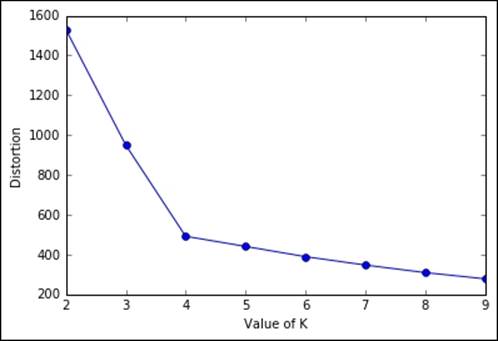
As you can expect, the distortion drops till K=4, then it decreases slowly. Here, the best-obtained K is 4.

Another unsupervised metric that we're going to see is the Silhouette. It's more complex, but also more powerful than the previous heuristics. At a very high level, it measures how close (similar) an observation is to the assigned cluster and how loosely (dissimilarly) it is matched to the data of nearby clusters. A Silhouette score of 1 indicates that all the data is in the best cluster, and -1 indicates a completely wrong cluster result. To obtain such a measure using Python code is very easy, thanks to the Scikit-learn implementation:

In:from sklearn.metrics import silhouette_score

Ks = range(2, 10)

Ds = []

for K in Ks:

cls = KMeans(n_clusters=K, random_state=101)

Ds.append(silhouette_score(X, cls.fit_predict(X)))

plt.plot(Ks, Ds, 'o-')

plt.xlabel("Value of K")

plt.ylabel("Silhouette score")

plt.show()

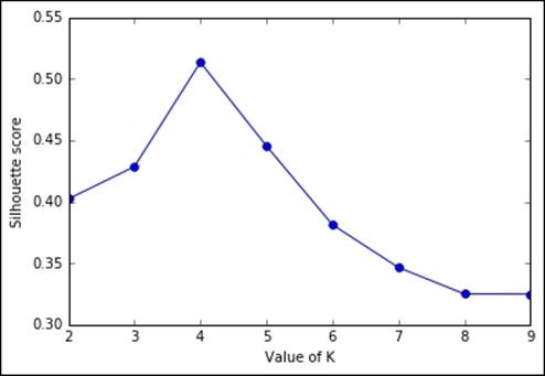
Even in this case, we've arrived at the same conclusion: the best value for K is 4 as the silhouette score is much lower with a lower and higher K.

Scaling K-means – mini-batch

Let's now test the scalability of K-means. From the website of UCI, we've selected an appropriate dataset for this task: the US Census 1990 Data. This dataset contains almost 2.5 million observations and 68 categorical (but already number-encoded) attributes. There is no missing data and the file is in the CSV format. Each observation contains the ID of the individual (to be removed before the clustering) and other information about gender, income, marital status, work, and so on.

Note

Further information about the dataset can be found at http://archive.ics.uci.edu/ml/datasets/US+Census+Data+%281990%29 or in the paper published in The Journal of Machine Learning Research by Meek, Thiesson, and Heckerman (2001) entitled The Learning Curve Method Applied to Clustering.

As the first thing to be done, you have to download the file containing the dataset and store it in a temporary directory. Note that it's 345MB in size, therefore its download might require a long time on slow connections:

In:import urllib

import os.path

url = "http://archive.ics.uci.edu/ml/machine-learning-databases/census1990-mld/USCensus1990.data.txt"

census_csv_file = "/tmp/USCensus1990.data.txt"

import os.path

if not os.path.exists(census_csv_file):

testfile = urllib.URLopener()

testfile.retrieve(url, census_csv_file)

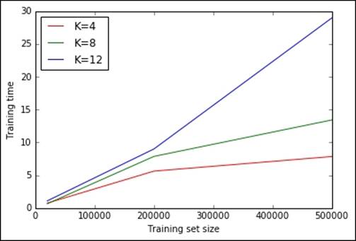
Now, let's run some tests clocking the times needed to train a K-means learner with K equal to 4, 8, and 12, and with a dataset containing 20K, 200K, and 0.5M observations. As we don't want to saturate the memory of the machine, consequently we will just read the first 500K lines and drop the column containing the identifier of the user. Finally, let's plot the training times for a complete performance evaluation:

In:piece_of_dataset = pd.read_csv(census_csv_file, iterator=True).get_chunk(500000).drop('caseid', axis=1).as_matrix()

time_results = {4: [], 8:[], 12:[]}

dataset_sizes = [20000, 200000, 500000]

for dataset_size in dataset_sizes:

print "Dataset size:", dataset_size

X = piece_of_dataset[:dataset_size,:]

for K in [4, 8, 12]:

print "K:", K

cls = KMeans(K, random_state=101)

timeit = %timeit -o -n1 -r1 cls.fit(X)

time_results[K].append(timeit.best)

plt.plot(dataset_sizes, time_results[4], 'r', label='K=4')

plt.plot(dataset_sizes, time_results[8], 'g', label='K=8')

plt.plot(dataset_sizes, time_results[12], 'b', label='K=12')

plt.xlabel("Training set size")

plt.ylabel("Training time")

plt.legend(loc=0)

plt.show()

Out:Dataset size: 20000

K: 4

1 loops, best of 1: 478 ms per loop

K: 8

1 loops, best of 1: 1.22 s per loop

K: 12

1 loops, best of 1: 1.76 s per loop

Dataset size: 200000

K: 4

1 loops, best of 1: 6.35 s per loop

K: 8

1 loops, best of 1: 10.5 s per loop

K: 12

1 loops, best of 1: 17.7 s per loop

Dataset size: 500000

K: 4

1 loops, best of 1: 13.4 s per loop

K: 8

1 loops, best of 1: 48.6 s per loop

K: 12

1 loops, best of 1: 1min 5s per loop

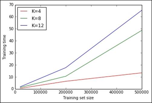
It seems clear that, given the plot and actual timings, the training time increases linearly with K and the training set size, but for large Ks and training sizes, such a relation becomes nonlinear. Doing an exhaustive search with the whole training set for many Ks does not seem scalable.

Fortunately, there's an online version of K-means based on mini-batches, already implemented in Scikit-learn and named MiniBatchKMeans. Let's try it on the slowest case of the previous cell, that is, with K=12. With the classic K-means, the training on 500,000 samples (circa 20% of the full dataset) took more than a minute; let's see the performance of the online mini-batch version, setting the batch size to 1,000 and importing chunks of 50,000 observations from the dataset. As an output, we plot the training time versus the number of chunks already passed thought the training phase:

In:from sklearn.cluster import MiniBatchKMeans

import time

cls = MiniBatchKMeans(12, batch_size=1000, random_state=101)

ts = []

tik = time.time()

for chunk in pd.read_csv(census_csv_file, chunksize=50000):

cls.partial_fit(chunk.drop('caseid', axis=1))

ts.append(time.time()-tik)

plt.plot(range(len(ts)), ts)

plt.xlabel('Training batches')

plt.ylabel('time [s]')

plt.show()

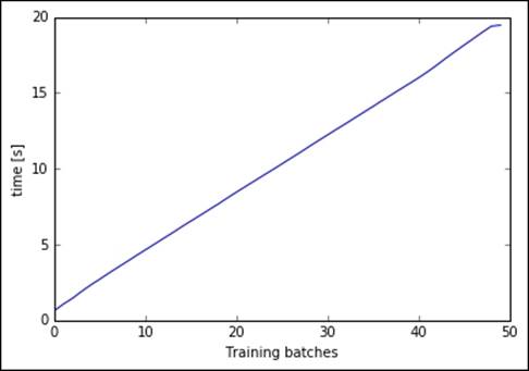
Training time is linear for each chunk, performing the clustering on the full 2.5 million observations dataset in nearly 20 seconds. With this implementation, we can run a full search to select the best K using the elbow method on the distortion. Let's do a gridsearch, with K spanning from 4 to 12, and plot the distortion:

In:Ks = list(range(4, 13))

ds = []

for K in Ks:

cls = MiniBatchKMeans(K, batch_size=1000, random_state=101)

for chunk in pd.read_csv(census_csv_file, chunksize=50000):

cls.partial_fit(chunk.drop('caseid', axis=1))

ds.append(cls.inertia_)

plt.plot(Ks, ds)

plt.xlabel('Value of K')

plt.ylabel('Distortion')

plt.show()

Out:

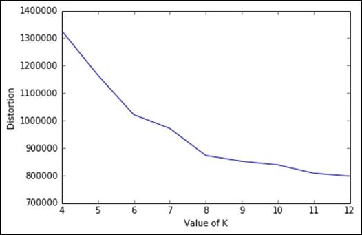
From the plot, the elbow seems in correspondence of K=8. Beyond the value, we would like to point out that in less than a couple of minutes, we've been able to perform this massive operation on a large dataset, thanks to the batch implementation; therefore remember never to use the plain vanilla K-means if the dataset is getting big.

K-means with H2O

Here, we're comparing the K-means implementation of H2O with Scikit-learn. More specifically, we will run the mini-batch experiment using H2OKMeansEstimator, the object for K-means available in H2O. The setup is similar to the one shown in the PCA with H2Osection, and the experiment is the same as seen in the preceding section:

In:import h2o

from h2o.estimators.kmeans import H2OKMeansEstimator

h2o.init(max_mem_size_GB=4)

def testH2O_kmeans(X, k):

temp_file = tempfile.NamedTemporaryFile().name

np.savetxt(temp_file, np.c_[X], delimiter=",")

cls = H2OKMeansEstimator(k=k, standardize=True)

blobdata = h2o.import_file(temp_file)

tik = time.time()

cls.train(x=range(blobdata.ncol), training_frame=blobdata)

fit_time = time.time() - tik

os.remove(temp_file)

return fit_time

piece_of_dataset = pd.read_csv(census_csv_file, iterator=True).get_chunk(500000).drop('caseid', axis=1).as_matrix()

time_results = {4: [], 8:[], 12:[]}

dataset_sizes = [20000, 200000, 500000]

for dataset_size in dataset_sizes:

print "Dataset size:", dataset_size

X = piece_of_dataset[:dataset_size,:]

for K in [4, 8, 12]:

print "K:", K

fit_time = testH2O_kmeans(X, K)

time_results[K].append(fit_time)

plt.plot(dataset_sizes, time_results[4], 'r', label='K=4')

plt.plot(dataset_sizes, time_results[8], 'g', label='K=8')

plt.plot(dataset_sizes, time_results[12], 'b', label='K=12')

plt.xlabel("Training set size")

plt.ylabel("Training time")

plt.legend(loc=0)

plt.show()

testH2O_kmeans(100000, 100)

h2o.shutdown(prompt=False)

Out:

Thanks to the H2O architecture, its implementation of K-means is very fast and scalable and able to perform the clustering of the 500K point datasets in less than 30 seconds for all the selected Ks.

LDA

LDA stands for Latent Dirichlet Allocation, and it's one of the widely-used techniques to analyze collections of textual documents.

Note

LDA is an acronym also used by another technique, Linear Discriminant Analysis, which is a supervised method for classification. Pay attention to how LDA is used as there's no connection between these two algorithms.

A full mathematical explanation of LDA would require the knowledge of probabilistic modeling, which is beyond the scope of this practical book. Here, instead, we will give you the most important intuitions behind the model and how to practically apply this model on a massive dataset.

First at all, LDA is used in a branch of data science named text mining, where the focus is on building learners to understand the natural language, for instance, based on textual examples. Specifically, LDA belongs to the category of topic-modeling algorithms as it tries to model the topics included in a document. Ideally, LDA is able to understand whether a document is about finance, politics, or religion, for example. However, differently from a classifier, it is also able to quantify the presence of topics in a document. For example, let's think about a Harry Potter novel, by Rowling. A classifier would be able to assess its category (fantasy novel); LDA, instead, is able to understand how much comedy, drama, mystery, romance, and adventure is in there. Moreover, LDA doesn't require any label; it's an unsupervised method and internally builds the output categories or topic and its composition (that is, given by the set of words composing a topic).

During the processing, LDA builds both a topics-per-document model and a words-per-topic model, modeled as Dirichlet distributions. Although the complexity is high, the processing time needed to output stable results is not all that long, thanks to an iterative Monte Carlo-like core function.

The LDA model is easy to understand: each document is modeled as a distribution of topics, and each topic is modeled as a distribution of words. Distributions assume to have a Dirichlet prior (with different parameters as the number of words per topic are usually different than the number of topics per document). Thanks to Gibbs sampling, distributions shouldn't be directly sampled, but an accurate approximate of it is obtained iteratively. Similar results can be obtained using the variational Bayes technique, where the approximation is generated with an Expectation-Maximization approach.

The resulting LDA model is generative (as happens with Hidden Markov Models, Naïve Bayes, and Restricted Boltzmann Machines), therefore each variable can be simulated and observed.

Let's now see how it works on a real-world dataset—the 20 Newsgroup dataset. It's composed of a collection of e-mails exchanged in 20 newsgroups. Let's initially load it, removing the e-mail headers, footers, and quotes from replied e-mails:

In:from sklearn.datasets import fetch_20newsgroups

documents = fetch_20newsgroups(remove=('headers', 'footers', \

'quotes'), random_state=101).data

Check the size of the dataset (that is, how many documents), and print one of them to see what one document is actually composed of:

In:len(documents)

Out:11314

In:document_num = 9960

print documents[document_num]

Out:Help!!!

I have an ADB graphicsd tablet which I want to connect to my

Quadra 950. Unfortunately, the 950 has only one ADB port and

it seems I would have to give up my mouse.

Please, can someone help me? I want to use the tablet as well as

the mouse (and the keyboard of course!!!).

Thanks in advance.

As in the example, one guy is looking for help for his video socket on his tablet.

Now, we import the Python packages needed to run LDA. The Gensim package is one of the best ones and, as you'll see at the end of the section, it is also very scalable:

In:import gensim

from gensim.utils import simple_preprocess

from gensim.parsing.preprocessing import STOPWORDS

from nltk.stem import WordNetLemmatizer, SnowballStemmer

np.random.seed(101)

As the first step, we should clean the text. A few steps are necessary, which is typical of any NLP text processing:

1. Tokenization is where the text is split into sentences and sentences are split into words. Finally, words are lowercased. At this point, punctuation (and accents) is removed.

2. Words composed of fewer than three characters are removed. (This step removes most of the acronyms, emoticons, and conjunctions.)

3. Words appearing in the list of English stopwords are removed. Words in this list are very common and have no predictive power (such as the, an, so, then, have, and so on).

4. Tokens are then lemmatized; words in third-person are changed to first-person, and verbs in past and future tenses are changed into present (for example, goes, went, and gone all become go).

5. Finally, stemming removes the inflection, reducing the word to its root (for example, shoes becomes shoe).

In the following piece of code, we will do exactly this: try to clean the text as much as possible and list the words composing each of them. At the end of the cell, we see how this operation changes the document seen previously:

In:lm = WordNetLemmatizer()

stemmer = SnowballStemmer("english")

def lem_stem(text):

return stemmer.stem(lm.lemmatize(text, pos='v'))

def tokenize_lemmatize(text):

return [lem_stem(token)

for token in gensim.utils.simple_preprocess(text)

if token not in gensim.parsing.preprocessing.STOPWORDS and len(token) > 3]

print tokenize_lemmatize(documents[document_num])

Out:[u'help', u'graphicsd', u'tablet', u'want', u'connect', u'quadra', u'unfortun', u'port', u'mous', u'help', u'want', u'tablet', u'mous', u'keyboard', u'cours', u'thank', u'advanc']

Now, as the next step, let's operate the cleaning steps on all the documents. After this, we have to build a dictionary containing how many times a word appears in the training set. Thanks to the Gensim package, this operation is straightforward:

In:processed_docs = [tokenize(doc) for doc in documents]

word_count_dict = gensim.corpora.Dictionary(processed_docs)

Now, as we want to build a generic and fast solution, let's remove all the very rare and very common words. For example, we can filter out all the words appearing less than 20 times (in total) and in no more than 20% of the documents:

In:word_count_dict.filter_extremes(no_below=20, no_above=0.2)

As the next step, with such a reduced set of words, we now build the bag-of-words model for each document; that is, for each document, we create a dictionary reporting how many words and how many times the words appear:

In:bag_of_words_corpus = [word_count_dict.doc2bow(pdoc) \

for pdoc in processed_docs]

As an example, let's have a peek at the bag-of-words model of the preceding document:

In:bow_doc1 = bag_of_words_corpus[document_num]

for i in range(len(bow_doc1)):

print "Word {} (\"{}\") appears {} time[s]" \

.format(bow_doc1[i][0], \

word_count_dict[bow_doc1[i][0]], bow_doc1[i][1])

Out:Word 178 ("want") appears 2 time[s]

Word 250 ("keyboard") appears 1 time[s]

Word 833 ("unfortun") appears 1 time[s]

Word 1037 ("port") appears 1 time[s]

Word 1142 ("help") appears 2 time[s]

Word 1543 ("quadra") appears 1 time[s]

Word 2006 ("advanc") appears 1 time[s]

Word 2124 ("cours") appears 1 time[s]

Word 2391 ("thank") appears 1 time[s]

Word 2898 ("mous") appears 2 time[s]

Word 3313 ("connect") appears 1 time[s]

Now, we have arrived at the core part of the algorithm: running LDA. As for our decision, let's ask for 12 topics (there are 20 different newsletters, but some are similar):

In:lda_model = gensim.models.LdaMulticore(bag_of_words_corpus, num_topics=10, id2word=word_count_dict, passes=50)

Note

If you get an error with such a code, try to mono-process the version with the gensim.models.LdaModel class instead of gensim.models.LdaMulticore.

Let's now print the topic composition, that is, the words appearing in each topic and their relative weight:

In:for idx, topic in lda_model.print_topics(-1):

print "Topic:{} Word composition:{}".format(idx, topic)

print

Out:

Topic:0 Word composition:0.015*imag + 0.014*version + 0.013*avail + 0.013*includ + 0.013*softwar + 0.012*file + 0.011*graphic + 0.010*program + 0.010*data + 0.009*format

Topic:1 Word composition:0.040*window + 0.030*file + 0.018*program + 0.014*problem + 0.011*widget + 0.011*applic + 0.010*server + 0.010*entri + 0.009*display + 0.009*error

Topic:2 Word composition:0.011*peopl + 0.010*mean + 0.010*question + 0.009*believ + 0.009*exist + 0.008*encrypt + 0.008*point + 0.008*reason + 0.008*post + 0.007*thing

Topic:3 Word composition:0.010*caus + 0.009*good + 0.009*test + 0.009*bike + 0.008*problem + 0.008*effect + 0.008*differ + 0.008*engin + 0.007*time + 0.006*high

Topic:4 Word composition:0.018*state + 0.017*govern + 0.015*right + 0.010*weapon + 0.010*crime + 0.009*peopl + 0.009*protect + 0.008*legal + 0.008*control + 0.008*drug

Topic:5 Word composition:0.017*christian + 0.016*armenian + 0.013*jesus + 0.012*peopl + 0.008*say + 0.008*church + 0.007*bibl + 0.007*come + 0.006*live + 0.006*book

Topic:6 Word composition:0.018*go + 0.015*time + 0.013*say + 0.012*peopl + 0.012*come + 0.012*thing + 0.011*want + 0.010*good + 0.009*look + 0.009*tell

Topic:7 Word composition:0.012*presid + 0.009*state + 0.008*peopl + 0.008*work + 0.008*govern + 0.007*year + 0.007*israel + 0.007*say + 0.006*american + 0.006*isra

Topic:8 Word composition:0.022*thank + 0.020*card + 0.015*work + 0.013*need + 0.013*price + 0.012*driver + 0.010*sell + 0.010*help + 0.010*mail + 0.010*look

Topic:9 Word composition:0.019*space + 0.011*inform + 0.011*univers + 0.010*mail + 0.009*launch + 0.008*list + 0.008*post + 0.008*anonym + 0.008*research + 0.008*send

Topic:10 Word composition:0.044*game + 0.031*team + 0.027*play + 0.022*year + 0.020*player + 0.016*season + 0.015*hockey + 0.014*leagu + 0.011*score + 0.010*goal

Topic:11 Word composition:0.075*drive + 0.030*disk + 0.028*control + 0.028*scsi + 0.020*power + 0.020*hard + 0.018*wire + 0.015*cabl + 0.013*instal + 0.012*connect

Unfortunately, LDA doesn't provide a name for each topic; we should do it manuall yourselves, based on our interpretation of the results of the algorithm. After having carefully examined the composition, we can name the discovered topics as follows:

Let's now try to understand what topics are represented in the preceding document and their weights:

In:

for index, score in sorted( \

lda_model[bag_of_words_corpus[document_num]], \

key=lambda tup: -1*tup[1]):

print "Score: {}\t Topic: {}".format(score, lda_model.print_topic(index, 10))

Out:Score: 0.938887758964 Topic: 0.022*thank + 0.020*card + 0.015*work + 0.013*need + 0.013*price + 0.012*driver + 0.010*sell + 0.010*help + 0.010*mail + 0.010*look

The highest score is associated with the topic PC Devices. Based on our previous knowledge of the collections of documents, it seems that the topic extraction has performed quite well.

Now, let's evaluate the model as a whole. The perplexity (or its logarithm) provides us with a metric to understand how well LDA has performed on the training dataset:

In:print "Log perplexity of the model is", lda_model.log_perplexity(bag_of_words_corpus)

Out:Log perplexity of the model is -7.2985188569

In this case, the perplexity is 2-7.298, and it's connected to the (log) likelihood that the LDA model is able to generate the documents in the test set, given the distribution of topics for those documents. The lower the perplexity, the better the model, because it basically means that the model can regenerate the text quite well.

Now, let's try to use the model on an unseen document. For simplicity, the document contains only the sentences, Golf or tennis? Which is the best sport to play?:

In:unseen_document = "Golf or tennis? Which is the best sport to play?"

bow_vector = word_count_dict.doc2bow(\

tokenize_lemmatize(unseen_document))

for index, score in sorted(lda_model[bow_vector], \

key=lambda tup: -1*tup[1]):

print "Score: {}\t Topic: {}".format(score, \

lda_model.print_topic(index, 5))

Out:Score: 0.610691655136 Topic: 0.044*game + 0.031*team + 0.027*play + 0.022*year + 0.020*player

Score: 0.222640440339 Topic: 0.018*state + 0.017*govern + 0.015*right + 0.010*weapon + 0.010*crime

As expected, the topic with a higher score is the one about "Games", followed by others with a relatively smaller score.

How does LDA scale with the size of the corpus? Fortunately, very well; the algorithm is iterative and allows online learning, similar to the mini-batch one. The key for the online process is the .update() method offered by LdaModel (or LdaMulticore).

We will do this test on a subset of the original corpus composed of the first 1,000 documents, and we will update our LDA model with batches of 50, 100, 200, and 500 documents. For each mini-batch updating the model, we will record the time and plot them on a graph:

In:small_corpus = bag_of_words_corpus[:1000]

batch_times = {}

for batch_size in [50, 100, 200, 500]:

print "batch_size =", batch_size

tik0 = time.time()

lda_model = gensim.models.LdaModel(num_topics=12, \

id2word=word_count_dict)

batch_times[batch_size] = []

for i in range(0, len(small_corpus), batch_size):

lda_model.update(small_corpus[i:i+batch_size], \

update_every=25, \

passes=1+500/batch_size)

batch_times[batch_size].append(time.time() - tik0)

Out:batch_size = 50

batch_size = 100

batch_size = 200

batch_size = 500

Note that we've set the update_every and passes parameters in the model update. This is necessary to make the model converge at each iteration and not return a non-converging model. Note that 500 has been chosen heuristically; if you set it lower, you'll have many warnings from Gensim about the non-convergence of the model.

Let's now plot the results:

In:plt.plot(range(50, 1001, 50), batch_times[50], 'g', \

label='size 50')

plt.plot(range(100, 1001, 100), batch_times[100], 'b', \

label='size 100')

plt.plot(range(200, 1001, 200), batch_times[200], 'k', \

label='size 200')

plt.plot(range(500, 1001, 500), batch_times[500], 'r', \

label='size 500')

plt.xlabel("Training set size")

plt.ylabel("Training time")

plt.xlim([0, 1000])

plt.legend(loc=0)

plt.show()

Out:

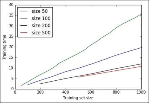
The bigger the batch, the faster the training. (Remember that big batches need fewer passes while updating the model.) On the other hand, the bigger the batch, the greater the amount of memory you need in order to store and process the corpora. Thanks to the mini-batches update method, LDA is able to scale to process a corpora of million documents. In fact, the implementation provided by the Gensim package is able to scale and process the whole of Wikipedia in a couple of hours on a domestic computer. If you're brave enough to try it yourself, here are the complete instructions to accomplish the task, provided by the author of the package:

https://radimrehurek.com/gensim/wiki.html

Scaling LDA – memory, CPUs, and machines

Gensim is very flexible and built to crunch big textual corpora; in fact, this library is able to scale without any modification or additional download:

1. With the number of CPUs, allowing parallel processes on a single node (with the classes, as seen in the first example).

2. With the number of observations, allowing online learning based on mini-batches. This can be achieved with the update method available in LdaModel and LdaMulticore (as shown in the previous example).

3. Running it on a cluster, distributing the workload across the nodes in the cluster, thanks to the Python library Pyro4 and the models.lda_dispatcher (as a scheduler) and models.lda_worker (as a worker process) objects, both provided by Gensim.

Beyond the classical LDA algorithm, Gensim also provides its hierarchical version, named Hierarchical Dirichlet Processing (HDP). Using this algorithm, topics follow a multilevel structure, enabling the user to understand complex corpora better (that is, where some documents are generic and some specific on a topic). This module is fairly new and, as of the end of 2015, not as scalable as the classic LDA.

Summary

In this chapter, we've introduced three popular unsupervised learners able to scale to cope with big data. The first, PCA, is able to reduce the number of features by creating ones containing the majority of variance (that is, the principal ones). K-means is a clustering algorithm able to group similar points together and associate them with a centroid. LDA is a powerful method to do topic modeling on textual data, that is, model the topics per document and the words appearing in a topic jointly.

In the next chapter, we will introduce some advanced and very recent methods of machine learning, still not part of the mainstream, naturally great for small datasets, but also suitable to process large scale machine learning.