Large Scale Machine Learning with Python (2016)
Chapter 8. Distributed Environments - Hadoop and Spark
In this chapter, we will introduce a new way to process data, scaling horizontally. So far, we've focused our attention primarily on processing big data on a standalone machine; here, we will introduce some methods that run on a cluster of machines.
Specifically, we will first illustrate the motivations and circumstances when we need a cluster to process big data. Then, we will introduce the Hadoop framework and all its components with a few examples (HDFS, MapReduce, and YARN), and finally, we will introduce the Spark framework and its Python interface—pySpark.
From a standalone machine to a bunch of nodes
The amount of data stored in the world is increasing exponentially. Nowadays, for a data scientist, having to process a few Terabytes of data a day is not an unusual request. To make things more complex, usually data comes from many different heterogeneous systems and the expectation of business is to produce a model within a short time.
Handling big data, therefore, is not just a matter of size, it's actually a three-dimensional phenomenon. In fact, according to the 3V model, systems operating on big data can be classified using three (orthogonal) criteria:
1. The first criterion is the velocity that the system archives to process the data. Although a few years ago, speed was indicating how quickly a system was able to process a batch; nowadays, velocity indicates whether a system can provide real-time outputs on streaming data.
2. The second criterion is volume, that is, how much information is available to be processed. It can be expressed in number of rows, features, or just a bare count of the bytes. To stream data, volume indicates the throughput of data arriving in the system.
3. The last criterion is variety, that is, the type of data sources. A few years ago, variety was limited by structured datasets; nowadays, data can be structured (tables, images, and so on), semi-structured (JSON, XML, and so on), and unstructured (webpages, social data, and so on). Usually, big data systems try to process as many relevant sources as possible, mixing all kinds of sources.
Beyond these criteria, many other Vs have appeared in the last years, trying to explain other features of big data. Some of these are as follows:
· Veracity (providing an indication of abnormality, bias, and noise contained in the data; ultimately, its accuracy)
· Volatility (indicating for how long the data can be used to extract meaningful information)
· Validity (the correctness of the data)
· Value (indicating the return over investment of the data)
In the recent years, all of the Vs have increased dramatically; now many companies have found that the data they retain has a huge value that can be monetized and they want to extract information out of it. The technical challenge has moved to have enough storage and processing power in order to be able to extract meaningful insights quickly, at scale, and using different input data streams.
Current computers, even the newest and most expensive ones, have a limited amount of disk, memory, and CPU. It looks very hard to process terabytes (or petabytes) of information per day, producing a quick model. Moreover, a standalone server containing both data and processing software needs to be replicated; otherwise, it could become the single point of failure of the system.
The world of big data has therefore moved to clusters: they're composed by a variable number of not very expensive nodes and sit on a high-speed Internet connection. Usually, some clusters are dedicated to storing data (a big hard disk, little CPU, and low amount of memory), and others are devoted to processing the data (a powerful CPU, medium-to-big amount of memory, and small hard disk). Moreover, if a cluster is properly set, it can ensure reliability (no single point of failure) and high availability.
Pay attention that, when we store data in a distributed environment (like a cluster), we should also consider the limitation of the CAP theorem; in the system, we can just ensure two out of the following three properties:
· Consistency: All the nodes are able to deliver the same data at the same time to a client
· Availability: A client requesting data is guaranteed to always receive a response, for both succeeded and failed requests
· Partition tolerance: If the network experiences failures and all the nodes cannot be in contact, the system is able to keep working
Specifically, the following are the consequences of the CAP theorem:
· If you give up on consistency, you'll create an environment where data is distributed across the nodes, and even though the network experiences some problems, the system is still able to provide a response to each request, although it is not guaranteed that the response to the same question is the same (it can be inconsistent). Typical examples of this configuration are DynamoDB, CouchDB, and Cassandra.
· If you give up on availability, you'll create a distributed system that can fail to respond to a query. Examples of this class are distributed-cache databases such as Redis, MongoDb, and MemcacheDb.
· Lastly, if you vice up on partition tolerance, you fall in the rigid schema of relational databases that don't allow the network to be split. This category includes MySQL, Oracle, and SQL Server.
Why do we need a distributed framework?
The easiest way to build a cluster is to use some nodes as storage nodes and others as processing ones. This configuration seems very easy as we don't need a complex framework to handle this situation. In fact, many small clusters are exactly built in this way: a couple of servers handle the data (plus their replica) and another bunch process the data.
Although this may appear as a great solution, it's not often used for many reasons:
· It just works for embarrassingly parallel algorithms. If an algorithm requires a common area of memory shared among the processing servers, this approach cannot be used.
· If one or many storage nodes die, the data is not guaranteed to be consistent. (Think about a situation where a node and its replica dies at the same time or where a node dies just after a write operation which has not yet been replicated.
· If a processing node dies, we are not able to keep track of the process that it was executing, making it hard to resume the processing on another node.
· If the network experiences failures, it's very hard to predict the situation after it's back to normality.
Let's now compute what the probability of a node failure is. Is it so rare that we can discard it? Is it something more concrete that we shall always take into consideration? The solution is easy: let's take into consideration a 100-node cluster, where each node has a probability of 1% of failure (cumulative of hardware and software crash) in the first year. What's the probability that all of the 100 will survive the first year? Under the hypothesis that every server is independent (that is, each node can crash independently of all the others), it's simply a multiplication:
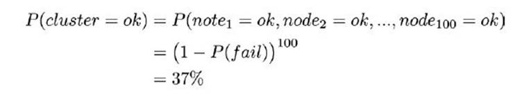
The result is very surprising at the beginning, but it explains why the big data community has put a lot of emphasis on the problem and developed many solutions for the cluster management in the past decade. From the formula's results, it seems that a crash event (or even more than one) is quite likely, a fact requiring that such an occurrence must be thought of in advance and handled properly to ensure the continuity of operations on the data. Furthermore, using cheap hardware or a bigger cluster, it looks almost certain that at least a node will fail.
Tip
The learning point here is that, once you go enterprise with big data, you must adopt enough countermeasures for node failures; it's the norm rather than the exception and should be handled properly to ensure the continuity of operations.
So far, the vast majority of cluster frameworks use the approach named divide et impera (split and conquer):
· There are modules specialized for the data nodes and some others specialized for data processing nodes (also named worker).
· Data is replicated across the data nodes, and one node is the master, ensuring that both the write and read operations succeed.
· The processing steps are split across the worker nodes. They don't share any state (unless stored in the data nodes) and their master ensures that all the tasks are performed positively and in the right order.
Note
Later on, we will introduce the Apache Hadoop framework in this chapter; although it is now a mature cluster management system, it still relies on solid foundations. Before that, let's set up the right working environment on our machines.
Setting up the VM
Setting up a cluster is a long and difficult operation; senior big data engineers earn their (high) salaries not just downloading and executing a binary application, but skillfully and carefully adapting the cluster manager to the desired working environment. It's a tough and complex operation; it may take a long time and if results are below the expectations, the whole business (including data scientists and software developers) won't be able to be productive. Data engineers must know every small detail of the nodes, data, operations that will be carried out, and network before starting to build the cluster. The output is usually a balanced, adaptive, fast, and reliable cluster, which can be used for years by all the technical people in the company.
Note
Is a cluster with a low number of very powerful nodes better than a cluster with many less powerful servers? The answer should be evaluated case-by-case, and it's highly dependent on the data, processing algorithms, number of people accessing it, speed at which we want the results, overall price, robustness of the scalability, network speed, and many other factors. Simply stated, it's not easy at all to decide for the best!
As setting up an environment is very difficult, we authors prefer to provide readers with a virtual machine image containing everything that you need in order to try some operations on a cluster. In the following sections, you'll learn how to set up a guest operating system on your machine, containing one node of a cluster with all the software you'd find on a real cluster.
Why only one node? As the framework that we've used is not lightweight, we decided to go for the atomic piece of a cluster ensuring that the environment you'll find in the node is exactly the same you'll find in a real-world situation. In order to run the virtual machine on your computer, you need two software: Virtualbox and Vagrant. Both of them are free of charge and open source.
VirtualBox
VirtualBox is an open source software used to virtualize one-to-many guest operative systems on Windows, macOS, and Linux host machines. From the user's point of view, a virtualized machine looks like another computer running in a window, with all its functionalities.
VirtualBox has become very popular because of its high performance, simplicity, and clean graphical user interface (GUI). Starting, stopping, importing, and terminating a virtual machine with VirtualBox is just a matter of a click.
Technically, VirtualBox is a hypervisor, which supports the creation and management of multiple virtual machines (VM) including many versions of Windows, Linux, and BSD-like distributions. The machine where VirtualBox runs is named host, while the virtualized machines are named guests. Note that there are no restrictions between the host and guests; for example, a Windows host can run Windows (the same version, a previous, or the most recent one) as well as any Linux and BSD distribution that is VirtualBox-compatible.
Virtualbox is often used to run software Operative-System specific; some software runs only on Windows or just a specific version of Windows, some is available only in Linux, and so on. Another application is to simulate new features on a cloned production environment; before trying the modifications in the live (production) environment, software developers usually test it on a clone, like one running on VirtualBox. Thanks to the guest isolation from the host, if something goes wrong in the guest (even formatting the hard disk), this doesn't impact the host. To have it back, just clone your machine before doing anything dangerous; you'll always be in time to recover it.
For those who want to start from scratch, VirtualBox supports virtual hard drives (including hard disks, CDs, DVDs, and floppy disks); this makes the installation of a new OS very simple. For example, if you want to install a plain vanilla version of Linux Ubuntu 14.04, you first download the .iso file. Instead of burning it on a CD/DVD, you can simply add it as a virtual drive to VirtualBox. Then, thanks to the simple step-by-step interface, you can select the hard drive size and the features of the guest machine (RAM, number of CPUs, video memory, and network connectivity). When operating with real bios, you can select the boot order: selecting the CD/DVD as a higher priority, you can start the process of the installation of Ubuntu as soon as you turn on the guest.
Now, let's download VirtualBox; remember to select the right version for your operating system.
Note
To install it on your computer, follow the instructions at https://www.virtualbox.org/wiki/Downloads.
At the time of writing this, the latest version is 5.1. Once installed, the graphical interface looks like the one in the following screenshot

We strongly advise you to take a look at how to set up a guest machine on your machine. Each guest machine will appear on the left-hand side of the window. (In the image, you can see that, on our computer, we have three stopped guests.) By clicking on each of them, on the right side will appear the detailed description of the virtualized hardware. In the example image, if the virtual machine named sparkbox_test (the one highlighted on the left) is turned on, it will be run on a virtual computer whose hardware is composed by a 4GB RAM, two processors, 40GB hard drive, and a video card with 12MB of RAM attached to the network with NAT.
Vagrant
Vagrant is a software that configures virtual environments at a high level. The core piece of Vagrant is the scripting capability, often used to create programmatically and automatically specific virtual environments. Vagrant uses VirtualBox (but also other virtualizers) to build and configure the virtual machines.
Note
To install it, follow the instructions at https://www.vagrantup.com/downloads.html.
Using the VM
With Vagrant and VirtualBox installed, you're now ready to run the node of a cluster environment. Create an empty directory and insert the following Vagrant commands into a new file named Vagrantfile:
Vagrant.configure("2") do |config|
config.vm.box = "sparkpy/sparkbox_test_1"
config.vm.hostname = "sparkbox"
config.ssh.insert_key = false
# Hadoop ResourceManager
config.vm.network :forwarded_port, guest: 8088, host: 8088, auto_correct: true
# Hadoop NameNode
config.vm.network :forwarded_port, guest: 50070, host: 50070, auto_correct: true
# Hadoop DataNode
config.vm.network :forwarded_port, guest: 50075, host: 50075, auto_correct: true
# Ipython notebooks (yarn and standalone)
config.vm.network :forwarded_port, guest: 8888, host: 8888, auto_correct: true
# Spark UI (standalone)
config.vm.network :forwarded_port, guest: 4040, host: 4040, auto_correct: true
config.vm.provider "virtualbox" do |v|
v.customize ["modifyvm", :id, "--natdnshostresolver1", "on"]
v.customize ["modifyvm", :id, "--natdnsproxy1", "on"]
v.customize ["modifyvm", :id, "--nictype1", "virtio"]
v.name = "sparkbox_test"
v.memory = "4096"
v.cpus = "2"
end
end
From top to bottom, the first lines download the right virtual machine (that we authors created and uploaded on a repository). Then, we set some ports to be forwarded to the guest machine; in this way, you'll be able to access some webservices of the virtualized machine. Finally, we set the hardware of the node.
Note
The configuration is set for a virtual machine with exclusive use of 4GB RAM and two cores. If your system can't meet these requirements, modify v.memory and v.cpus values to those good for your machine. Note that some of the following code examples may fail if the configuration that you set is not adequate.
Now, open a terminal and navigate to the directory containing the Vagrantfile. Here, launch the virtual machine with the following command:
$ vagrant up
The first time, this command will take a while as it downloads (it's an almost 2GB download) and builds the correct structure of the virtual machine. The next time, this command takes a smaller amount of time as there is nothing more to download.
After having turned on the virtual machine on your local system, you can access it as follows:
$ vagrant ssh
This command simulates an SSH access, and you'll be inside the virtualized machine finally.
Note
On Windows machines, this command may fail with an error due to the missing SSH executable. In such a situation, download and install an SSH client for Windows, such as Putty (http://www.putty.org/), Cygwin openssh (http://www.cygwin.com/), or Openssh for Windows (http://sshwindows.sourceforge.net/). Unix systems should not be affected by this problem.
To turn if off, you first need to exit the machine. From inside the VM, simply use the exit command to exit the SSH connection and then shut down the VM:
$ vagrant halt
Note
The virtual machine consumes resources. Remember to turn it off when you're done with the work with the vagranthalt command from the directory where the VM is located.
The preceding command shuts down the virtual machine, exactly as you would do with a server. To remove it and delete all its content, use the vagrant destroy command. Use it carefully: after having destroyed the machine, you won't be able to recover the files in there.
Here are the instructions to use IPython (Jupyter) Notebook inside the virtual machine:
1. Launch vagrant up and vagrant ssh from the folder containing the Vagrantfile. You should now be inside the virtual machine.
2. Now, launch the script:
3. vagrant@sparkbox:~$ ./start_hadoop.sh
4. At this point, launch the following shell script:
5. vagrant@sparkbox:~$ ./start_jupyter_yarn.sh
Open a browser on your local machine and point it to http://localhost:8888.
Here is the notebook that's backed by the cluster node. To turn the notebook and virtual machine off, perform the following steps:
1. To terminate the Jupyter console, press Ctrl + C (and then type Y for Yes).
2. Terminate the Hadoop framework as follows:
3. vagrant@sparkbox:~$ ./stop_hadoop.sh
4. Exit the virtual machine with the following command:
5. vagrant@sparkbox:~$ exit
6. Shut down the VirtualBox machine with vagrant halt.
The Hadoop ecosystem
Apache Hadoop is a very popular software framework for distributed storage and distributed processing on a cluster. Its strengths are in the price (it's free), flexibility (it's open source, and although being written in Java, it can by used by other programming languages), scalability (it can handle clusters composed by thousands of nodes), and robustness (it was inspired by a published paper from Google and has been around since 2011), making it the de facto standard to handle and process big data. Moreover, lots of other projects from the Apache foundation extend its functionalities.
Architecture
Logically, Hadoop is composed of two pieces: distributed storage (HDFS) and distributed processing (YARN and MapReduce). Although the code is very complex, the overall architecture is fairly easy to understand. A client can access both storage and processing through two dedicated modules; they are then in charge of distributing the job across all theorking nodes:
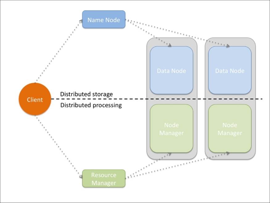
All the Hadoop modules run as services (or instances), that is, a physical or virtual node can run many of them. Typically, for small clusters, all the nodes run both distributed computing and processing services; for big clusters, it may be better to separate the two functionalities specializing the nodes.
We will see the functionalities offered by the two layers in detail.
HDFS
The Hadoop Distributed File System (HDFS) is a fault-tolerant distributed filesystem, designed to run on commodity low-cost hardware and able to handle very large datasets (in the order of hundred petabytes to exabytes). Although HDFS requires a fast network connection to transfer data across nodes, the latency can't be as low as in classic filesystems (it may be in the order of seconds); therefore, HDFS has been designed for batch processing and high throughput. Each HDFS node contains a part of the filesystem's data; the same data is also replicated in other instances and this ensures a high throughput access and fault-tolerance.
HDFS's architecture is master-slave. If the master (Name Node) fails, there is a secondary/backup one ready to take control. All the other instances are slaves (Data Nodes); if one of them fails, there's no problem as HDFS has been designed with this in mind.
Data Nodes contain blocks of data: each file saved in HDFS is broken up in chunks (or blocks), typically 64MB each, and then distributed and replicated in a set of Data Nodes.
The Name Node stores just the metadata of the files in the distributed filesystem; it doesn't store any actual data, but just the right indications on how to access the files in the multiple Data Nodes that it manages.
A client asking to read a file shall first contact the Name Node, which will give back a table containing an ordered list of blocks and their locations (as in Data Nodes). At this point, the client should contact the Data Nodes separately, downloading all the blocks and reconstructing the file (by appending the blocks together).
To write a file, instead, a client should first contact the Name Node, which will first decide how to handle the request, updating its records and then replying to the client with an ordered list of Data Nodes of where to write each block of the file. The client will now contact and upload the blocks to the Data Nodes, as reported in the Name Node reply.
Namespace queries (for example, listing a directory content, creating a folder, and so on) are instead completely handled by the Name Node by accessing its metadata information.
Moreover, Name Node is also responsible for handling a Data Node failure properly (it's marked as dead if no Heartbeat packets are received) and its data re-replication to other nodes.
Although these operations are long and hard to be implemented with robustness, they're completely transparent to the user, thanks to many libraries and the HDFS shell. The way you operate on HDFS is pretty similar to what you're currently doing on your filesystem and this is a great benefit of Hadoop: hiding the complexity and letting the user use it with simplicity.
Let's now take a look at the HDFS shell and later, a Python library.
Note
Use the preceding instructions to turn the VM on and launch the IPython Notebook on your computer.
Now, open a new notebook; this operation will take more time than usual as each notebook is connected to the Hadoop cluster framework. When the notebook is ready to be used, you'll see a flag saying Kernel starting, please wait … on the top right disappear.
The first piece is about the HDFS shell; therefore, all the following commands can be run at a prompt or shell of the virtualized machine. To run them in an IPython Notebook, all of them are anticipated by a question mark !, which is a short way to execute bash code in a notebook.
The common denominator of the following command lines is the executable; we will always run the hdfs command. It's the main interface to access and manage the HDFS system and the main command for the HDFS shell.
We start with a report on the state of HDFS. To obtain the details of the distributed filesystem (dfs) and its Data Nodes, use the dfsadmin subcommand:
In:!hdfs dfsadmin –report
Out:Configured Capacity: 42241163264 (39.34 GB)
Present Capacity: 37569168058 (34.99 GB)
DFS Remaining: 37378433024 (34.81 GB)
DFS Used: 190735034 (181.90 MB)
DFS Used%: 0.51%
Under replicated blocks: 0
Blocks with corrupt replicas: 0
Missing blocks: 0
-------------------------------------------------
Live datanodes (1):
Name: 127.0.0.1:50010 (localhost)
Hostname: sparkbox
Decommission Status : Normal
Configured Capacity: 42241163264 (39.34 GB)
DFS Used: 190735034 (181.90 MB)
Non DFS Used: 4668290330 (4.35 GB)
DFS Remaining: 37380775936 (34.81 GB)
DFS Used%: 0.45%
DFS Remaining%: 88.49%
Configured Cache Capacity: 0 (0 B)
Cache Used: 0 (0 B)
Cache Remaining: 0 (0 B)
Cache Used%: 100.00%
Cache Remaining%: 0.00%
Xceivers: 1
Last contact: Tue Feb 09 19:41:17 UTC 2016
The dfs subcommand allows using some well-known Unix commands to access and interact with the distributed filesystem. For example, list the content of the the root directory as follows:
In:!hdfs dfs -ls /
Out:Found 2 items
drwxr-xr-x - vagrant supergroup 0 2016-01-30 16:33 /spark
drwxr-xr-x - vagrant supergroup 0 2016-01-30 18:12 /user
The output is similar to the ls command provided by Linux, listing the permissions, number of links, user and group owning the file, size, timestamp of the last modification, and name for each file or directory.
Similar to the df command, we can invoke the -df argument to display the amount of available disk space in HDFS. The -h option will make the output more readable (using gigabytes and megabytes instead of bytes):
In:!hdfs dfs -df -h /
Out:Filesystem Size Used Available Use%
hdfs://localhost:9000 39.3 G 181.9 M 34.8 G 0%
Similar to du, we can use the -du argument to display the size of each folder contained in the root. Again, -h will produce a more human readable output:
In:!hdfs dfs -du -h /
Out:178.9 M /spark
1.4 M /user
So far, we've extracted some information from HDFS. Let's now do some operations on the distributed filesystem, which will modify it. We can start with creating a folder with the -mkdir option followed by the name. Note that this operation may fail if the directory already exists (exactly as in Linux, with the mkdir command):
In:!hdfs dfs -mkdir /datasets
Let's now transfer some files from the hard disk of the node to the distributed filesystem. In the VM that we've created, there is already a text file in the ../datasets directory; let's download a text file from the Internet. Let's move both of them to the HDFS directory that we've created with the previous command:
In:
!wget -q http://www.gutenberg.org/cache/epub/100/pg100.txt \
-O ../datasets/shakespeare_all.txt
!hdfs dfs -put ../datasets/shakespeare_all.txt \
/datasets/shakespeare_all.txt
!hdfs dfs -put ../datasets/hadoop_git_readme.txt \
/datasets/hadoop_git_readme.txt
Was the importing successful? Yes, we didn't have any errors. However, to remove any doubt, let's list the HDFS directory/datasets to see the two files:
In:!hdfs dfs -ls /datasets
Out:Found 2 items
-rw-r--r-- 1 vagrant supergroup 1365 2016-01-31 12:41 /datasets/hadoop_git_readme.txt
-rw-r--r-- 1 vagrant supergroup 5589889 2016-01-31 12:41 /datasets/shakespeare_all.txt
To concatenate some files to the standard output, we can use the -cat argument. In the following piece of code, we're counting the new lines appearing in a text file. Note that the first command is piped into another command that is operating on the local machine:
In:!hdfs dfs -cat /datasets/hadoop_git_readme.txt | wc –l
Out:30
Actually, with the -cat argument, we can concatenate multiple files from both the local machine and HDFS. To see it, let's now count how many newlines are present when the file stored on HDFS is concatenated to the same one stored on the local machine. To avoid misinterpretations, we can use the full Uniform Resource Identifier (URI), referring to the files in HDFS with the hdfs: scheme and to local files with the file: scheme:
In:!hdfs dfs -cat \
hdfs:///datasets/hadoop_git_readme.txt \
file:///home/vagrant/datasets/hadoop_git_readme.txt | wc –l
Out:60
In order to copy in HDFS, we can use the -cp argument:
In : !hdfs dfs -cp /datasets/hadoop_git_readme.txt \
/datasets/copy_hadoop_git_readme.txt
To delete a file (or directories, with the right option), we can use the –rm argument. In this snippet of code, we're removing the file that we've just created with the preceding command. Note that HDFS has the thrash mechanism; consequently, a deleted file is not actually removed from the HDFS but just moved to a special directory:
In:!hdfs dfs -rm /datasets/copy_hadoop_git_readme.txt
Out:16/02/09 21:41:44 INFO fs.TrashPolicyDefault: Namenode trash configuration: Deletion interval = 0 minutes, Emptier interval = 0 minutes.
Deleted /datasets/copy_hadoop_git_readme.txt
To empty the thrashed data, here's the command:
In:!hdfs dfs –expunge
Out:16/02/09 21:41:44 INFO fs.TrashPolicyDefault: Namenode trash configuration: Deletion interval = 0 minutes, Emptier interval = 0 minutes.
To obtain (get) a file from HDFS to the local machine, we can use the -get argument:
In:!hdfs dfs -get /datasets/hadoop_git_readme.txt \
/tmp/hadoop_git_readme.txt
To take a look at a file stored in HDFS, we can use the -tail argument. Note that there's no head function in HDFS as it can be done using cat and the result then piped in a local head command. As for the tail, the HDFS shell just displays the last kilobyte of data:
In:!hdfs dfs -tail /datasets/hadoop_git_readme.txt
Out:ntry, of
encryption software. BEFORE using any encryption software, please
check your country's laws, regulations and policies concerning the
import, possession, or use, and re-export of encryption software, to
see if this is permitted. See <http://www.wassenaar.org/> for more
information.
[...]
The hdfs command is the main entry point for HDFS, but it's slow and invoking system commands from Python and reading back the output is very tedious. For this, there exists a library for Python, Snakebite, which wraps many distributed filesystem operations. Unfortunately, the library is not as complete as the HDFS shell and is bound to a Name Node. To install it on your local machine, simply use pip install snakebite.
To instantiate the client object, we should provide the IP (or its alias) and the port of the Name Node. In the VM we provided, it's running on port 9000:
In:from snakebite.client import Client
client = Client("localhost", 9000)
To print some information about the HDFS, the client object has the serverdefaults method:
In:client.serverdefaults()
Out:{'blockSize': 134217728L,
'bytesPerChecksum': 512,
'checksumType': 2,
'encryptDataTransfer': False,
'fileBufferSize': 4096,
'replication': 1,
'trashInterval': 0L,
'writePacketSize': 65536}
To list the files and directories in the root, we can use the ls method. The result is a list of dictionaries, one for each file, containing information such as permissions, timestamp of the last modification, and so on. In this example, we're just interested in the paths (that is, the names):
In:for x in client.ls(['/']):
print x['path']
Out:/datasets
/spark
/user
Exactly as the preceding code, the Snakebite client has the du (for disk usage) and df (for disk free) methods available. Note that many methods (like du) return generators, which means that they need to be consumed (like an iterator or list) to be executed:
In:client.df()
Out:{'capacity': 42241163264L,
'corrupt_blocks': 0L,
'filesystem': 'hdfs://localhost:9000',
'missing_blocks': 0L,
'remaining': 37373218816L,
'under_replicated': 0L,
'used': 196237268L}
In:list(client.du(["/"]))
Out:[{'length': 5591254L, 'path': '/datasets'},
{'length': 187548272L, 'path': '/spark'},
{'length': 1449302L, 'path': '/user'}]
As for the HDFS shell example, we will now try to count the newlines appearing in the same file with Snakebite. Note that the .cat method returns a generator:
In:
for el in client.cat(['/datasets/hadoop_git_readme.txt']):
print el.next().count("\n")
Out:30
Let's now delete a file from HDFS. Again, pay attention that the delete method returns a generator and the execution never fails, even if we're trying to delete a non-existing directory. In fact, Snakebite doesn't raise exceptions, but just signals to the user in the output dictionary that the operation failed:
In:client.delete(['/datasets/shakespeare_all.txt']).next()
Out:{'path': '/datasets/shakespeare_all.txt', 'result': True}
Now, let's copy a file from HDFS to the local filesystem. Observe that the output is a generator, and you need to check the output dictionary to see if the operation was successful:
In:
(client
.copyToLocal(['/datasets/hadoop_git_readme.txt'],
'/tmp/hadoop_git_readme_2.txt')
.next())
Out:{'error': '',
'path': '/tmp/hadoop_git_readme_2.txt',
'result': True,
'source_path': '/datasets/hadoop_git_readme.txt'}
Finally, create a directory and delete all the files matching a string:
In:list(client.mkdir(['/datasets_2']))
Out:[{'path': '/datasets_2', 'result': True}]
In:client.delete(['/datasets*'], recurse=True).next()
Out:{'path': '/datasets', 'result': True}
Where is the code to put a file in HDFS? Where is the code to copy an HDFS file to another one? Well, these functionalities are not yet implemented in Snakebite. For them, we shall use the HDFS shell through system calls.
MapReduce
MapReduce is the programming model implemented in the earliest versions of Hadoop. It's a very simple model, designed to process large datasets on a distributed cluster in parallel batches. The core of MapReduce is composed of two programmable functions—a mapper that performs filtering and a reducer that performs aggregation—and a shuffler that moves the objects from the mappers to the right reducers.
Note
Google has published a paper in 2004 on Mapreduce, a few months after having been granted a patent on it.
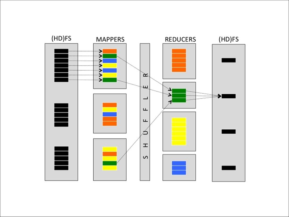
Specifically, here are the steps of MapReduce for the Hadoop implementation:
1. Data chunker. Data is read from the filesystem and split into chunks. A chunk is a piece of the input dataset, typically either a fixed-size block (for example, a HDFS block read from a Data Node) or another more appropriate split.
For example, if we want to count the number of characters, words, and lines in a text file, a nice split can be a line of text.
2. Mapper: From each chunk, a series of key-value pairs is generated. Each mapper instance applies the same mapping function on different chunks of data.
Continuing the preceding example, for each line, three key-value pairs are generated in this step—one containing the number of characters in the line (the key can simply be a chars string), one containing the number of words (in this case, the key must be different, let's say words), and one containing the number of lines, which is always one (in this case, the key can be lines).
3. Shuffler: From the key and number of available reducers, the shuffler distributes all the key-value pairs with the same key to the same reducers. Typically, this operation is the hash of the key, modulo the number of reducers. This should ensure a fair amount of keys for each reducer. This function is not user-programmable, but provided by the MapReduce framework.
4. Reducer: Each reducer receives all the key-value pairs for a specific set of keys and can produce zero or more aggregate results.
In the example, all the values connected to the words key arrive at a reducer; its job is just summing up all the values. The same happens for the other keys, resulting in three final values: the number of characters, number of words, and number of lines. Note that these results may be on different reducers.
5. Output writer: The outputs of the reducers are written on the filesystem (or HDFS). In the default Hadoop configuration, each reducer writes a file (part-r-00000 is the output of the first reducer, part-r-00001 of the second, and so on). To have a full list of results on a file, you should concatenate all of them.
Visually, this operation can be simply communicated and understood as follows:
There's also an optional step that can be run by each mapper instance after the mapping step—the combiner. It basically anticipates, if possible, the reducing step on the mapper and is often used to decrease the amount of information to shuffle, speeding up theprocess. In the preceding example, if a mapper processes more than one line of the input file, during the (optional) combiner step, it can pre-aggregate the results, outputting the smaller number of key-value pairs. For example, if the mapper processes 100 lines of text in each chunk, why output 300 key-value pairs (100 for the number of chars, 100 for words, and 100 for lines) when the information can be aggregated in three? That's actually the goal of the combiner.
In the MapReduce implementation provided by Hadoop, the shuffle operation is distributed, optimizing the communication cost, and it's possible to run more than one mapper and reducer per node, making full use of the hardware resources available on the nodes. Also, the Hadoop infrastructure provides redundancy and fault-tolerance as the same task can be assigned to multiple workers.
Let's now see how it works. Although the Hadoop framework is written in Java, thanks to the Hadoop Streaming utility, mappers and reducers can be any executable, including Python. Hadoop Streaming uses the pipe and standard inputs and outputs to stream the content; therefore, mappers and reducers must implement a reader from stdin and a key-value writer on stdout.
Now, turn on the virtual machine and open a new IPython notebook. Even in this case, we will first introduce the command line way to run MapReduce jobs provided by Hadoop, then introduce a pure Python library. The first example will be exactly what we've described: a counter of the number of characters, words, and lines of a text file.
First, let's insert the datasets into HDFS; we're going to use the Hadoop Git readme (a short text file containing the readme file distributed with Apache Hadoop) and the full text of all the Shakespeare books, provided by Project Gutenberg (although it's just 5MB, it contains almost 125K lines). In the first cell, we'll be cleaning up the folder from the previous experiment, then, we download the file containing the Shakespeare bibliography in the dataset folder, and finally, we put both datasets on HDFS:
In:!hdfs dfs -mkdir -p /datasets
!wget -q http://www.gutenberg.org/cache/epub/100/pg100.txt \
-O ../datasets/shakespeare_all.txt
!hdfs dfs -put -f ../datasets/shakespeare_all.txt /datasets/shakespeare_all.txt
!hdfs dfs -put -f ../datasets/hadoop_git_readme.txt /datasets/hadoop_git_readme.txt
!hdfs dfs -ls /datasets
Now, let's create the Python executable files containing the mapper and reducer. We will use a very dirty hack here: we're going to write Python files (and make them executable) using a write operation from the Notebook.
Both the mapper and reducer read from the stdin and write to the stdout (with simple print commands). Specifically, the mapper reads lines from the stdin and prints the key-value pairs of the number of characters (except the newline), the number of words (by splitting the line on the whitespace), and the number of lines, always one. The reducer, instead, sums up the values for each key and prints the grand total:
In:
with open('mapper_hadoop.py', 'w') as fh:
fh.write("""#!/usr/bin/env python
import sys
for line in sys.stdin:
print "chars", len(line.rstrip('\\n'))
print "words", len(line.split())
print "lines", 1
""")
with open('reducer_hadoop.py', 'w') as fh:
fh.write("""#!/usr/bin/env python
import sys
counts = {"chars": 0, "words":0, "lines":0}
for line in sys.stdin:
kv = line.rstrip().split()
counts[kv[0]] += int(kv[1])
for k,v in counts.items():
print k, v
""")
In:!chmod a+x *_hadoop.py
To see it at work, let's try it locally without using Hadoop. In fact, as mappers and reducers read and write to the standard input and output, we can just pipe all the things together. Note that the shuffler can be replaced by the sort -k1,1 command, which sorts the input strings using the first field (that is, the key):
In:!cat ../datasets/hadoop_git_readme.txt | ./mapper_hadoop.py | sort -k1,1 | ./reducer_hadoop.py
Out:chars 1335
lines 31
words 179
Let's now use the Hadoop MapReduce way to get the same result. First of all, we should create an empty directory in HDFS able to store the results. In this case, we create a directory named /tmp and we remove anything inside named in the same way as the job output (Hadoop will fail if the output file already exists). Then, we use the right command to run the MapReduce job. This command includes the following:
· The fact that we want to use the Hadoop Streaming capability (indicating the Hadoop streaming jar file)
· The mappers and reducers that we want to use (the –mapper and –reducer options)
· The fact that we want to distribute these files to each mapper as they're local files (with the –files option)
· The input file (the –input option) and the output directory (the –output option)
In:!hdfs dfs -mkdir -p /tmp
!hdfs dfs -rm -f -r /tmp/mr.out
!hadoop jar /usr/local/hadoop/share/hadoop/tools/lib/hadoop-streaming-2.6.4.jar \
-files mapper_hadoop.py,reducer_hadoop.py \
-mapper mapper_hadoop.py -reducer reducer_hadoop.py \
-input /datasets/hadoop_git_readme.txt -output /tmp/mr.out
Out:[...]
16/02/04 17:12:22 INFO mapreduce.Job: Running job: job_1454605686295_0003
16/02/04 17:12:29 INFO mapreduce.Job: Job job_1454605686295_0003 running in uber mode : false
16/02/04 17:12:29 INFO mapreduce.Job: map 0% reduce 0%
16/02/04 17:12:35 INFO mapreduce.Job: map 50% reduce 0%
16/02/04 17:12:41 INFO mapreduce.Job: map 100% reduce 0%
16/02/04 17:12:47 INFO mapreduce.Job: map 100% reduce 100%
16/02/04 17:12:47 INFO mapreduce.Job: Job job_1454605686295_0003 completed successfully
[...]
Shuffle Errors
BAD_ID=0
CONNECTION=0
IO_ERROR=0
WRONG_LENGTH=0
WRONG_MAP=0
WRONG_REDUCE=0
[...]
16/02/04 17:12:47 INFO streaming.StreamJob: Output directory: /tmp/mr.out
The output is very verbose; we just extracted three important sections in it. The first indicates the progress of the MapReduce job, and it's very useful to track and estimate the time needed to complete the operation. The second section highlights the errors, which may have occurred during the job, and the last section reports the output directory and timestamp of the termination. The whole process on the small file (of 30 lines) took almost half a minute! The reasons are very simple: first, Hadoop MapReduce has been designed for robust big data processing and contains a lot of overhead, and second, the ideal environment is a cluster of powerful machines, not a virtualized VM with 4GB of RAM. On the other hand, this code can be run on much bigger datasets and a cluster of a very powerful machine, without changing anything.
Let's not see the results immediately. First, let's take a peek at the output directory in HDFS:
In:!hdfs dfs -ls /tmp/mr.out
Out:Found 2 items
-rw-r--r-- 1 vagrant supergroup 0 2016-02-04 17:12 /tmp/mr.out/_SUCCESS
-rw-r--r-- 1 vagrant supergroup 33 2016-02-04 17:12 /tmp/mr.out/part-00000
There are two files: the first is empty and named _SUCCESS and indicates that the MapReduce job has finished the writing stage in the directory, and the second is named part-00000 and contains the actual results (as we're operating on a node with just one reducer). Reading this file will provide us with the final results:
In:!hdfs dfs -cat /tmp/mr.out/part-00000
Out:chars 1335
lines 31
words 179
As expected, they're the same as the piped command line shown previously.
Although conceptually simple, Hadoop Streaming is not the best way to run Hadoop jobs with Python code. For this, there are many libraries available on Pypy; the one we're presenting here is one of the most flexible and maintained open source one—MrJob. It allows you to run the jobs seamlessly on your local machine, your Hadoop cluster, or the same cloud cluster environments, such as Amazon Elastic MapReduce; it merges all the code in a standalone file even if multiple MapReduce steps are needed (think about iterative algorithms) and interprets Hadoop errors in the code. Also, it's very simple to install; to have the MrJob library on your local machine, simply use pip install mrjob.
Although MrJob is a great piece of software, it doesn't work very well with IPython Notebook as it requires a main function. Here, we need to write the MapReduce Python code in a separate file and then run a command line.
We start with the example that we've seen many times so far: counting characters, words, and lines in a file. First, let's write the Python file using the MrJob functionalities; mappers and reducers are wrapped in a subclass of MRJob. Inputs are not read from stdin, but passed as a function argument, and outputs are not printed, but yielded (or returned).
Thanks to MrJob, the whole MapReduce program becomes just a few lines of code:
In:
with open("MrJob_job1.py", "w") as fh:
fh.write("""
from mrjob.job import MRJob
class MRWordFrequencyCount(MRJob):
def mapper(self, _, line):
yield "chars", len(line)
yield "words", len(line.split())
yield "lines", 1
def reducer(self, key, values):
yield key, sum(values)
if __name__ == '__main__':
MRWordFrequencyCount.run()
""")
Let's now execute it locally (with the local version of the dataset).The MrJob library, beyond executing the mapper and reducer steps (locally, in this case), also prints the result and cleans up the temporary directory:
In:!python MrJob_job1.py ../datasets/hadoop_git_readme.txt
Out: [...]
Streaming final output from /tmp/MrJob_job1.vagrant.20160204.171254.595542/output
"chars" 1335
"lines" 31
"words" 179
removing tmp directory /tmp/MrJob_job1.vagrant.20160204.171254.595542
To run the same process on Hadoop, just run the same Python file, this time inserting the –r hadoop option in the command line, and automatically MrJob will execute it using Hadoop MapReduce and HDFS. In this case, remember to point the hdfs path of the input file:
In:
!python MrJob_job1.py -r hadoop hdfs:///datasets/hadoop_git_readme.txt
Out:[...]
HADOOP: Running job: job_1454605686295_0004
HADOOP: Job job_1454605686295_0004 running in uber mode : false
HADOOP: map 0% reduce 0%
HADOOP: map 50% reduce 0%
HADOOP: map 100% reduce 0%
HADOOP: map 100% reduce 100%
HADOOP: Job job_1454605686295_0004 completed successfully
[...]
HADOOP: Shuffle Errors
HADOOP: BAD_ID=0
HADOOP: CONNECTION=0
HADOOP: IO_ERROR=0
HADOOP: WRONG_LENGTH=0
HADOOP: WRONG_MAP=0
HADOOP: WRONG_REDUCE=0
[...]
Streaming final output from hdfs:///user/vagrant/tmp/mrjob/MrJob_job1.vagrant.20160204.171255.073506/output
"chars" 1335
"lines" 31
"words" 179
removing tmp directory /tmp/MrJob_job1.vagrant.20160204.171255.073506
deleting hdfs:///user/vagrant/tmp/mrjob/MrJob_job1.vagrant.20160204.171255.073506 from HDFS
You will see the same output of the Hadoop Streaming command line as seen previously, plus the results. In this case, the HDFS temporary directory, used to store the results, is removed after the termination of the job.
Now, to see the flexibility of MrJob, let's try running a process that requires more than one MapReduce Step. While done from the command line, this is a very difficult task; in fact, you have to run the first iteration of MapReduce, check the errors, read the results, and then launch the second iteration of MapReduce, check the errors again, and finally read the results. This sounds very time-consuming and prone to errors. Thanks to MrJob, this operation is very easy: within the code, it's possible to create a cascade of MapReduce operations, where each output is the input of the next stage.
As an example, let's now find the most common word used by Shakespeare (using, as input, the 125K lines file). This operation cannot be done in a single MapReduce step; it requires at least two of them. We will implement a very simple algorithm based on two iterations of MapReduce:
· Data chunker: Just as for the MrJob default, the input file is split on each line.
· Stage 1 – map: A key-map tuple is yielded for each word; the key is the lowercased word and the value is always 1.
· Stage 1 – reduce: For each key (lowercased word), we sum all the values. The output will tell us how many times the word appears in the text.
· Stage 2 – map: During this step, we flip the key-value tuples and put them as values of a new key pair. To force one reducer to have all the tuples, we assign the same key, None, to each output tuple.
· Stage 2 – reduce: We simply discard the only key available and extract the maximum of the values, resulting in extracting the maximum of all the tuples (count, word).
In:
with open("MrJob_job2.py", "w") as fh:
fh.write("""
from mrjob.job import MRJob
from mrjob.step import MRStep
import re
WORD_RE = re.compile(r"[\w']+")
class MRMostUsedWord(MRJob):
def steps(self):
return [
MRStep(mapper=self.mapper_get_words,
reducer=self.reducer_count_words),
MRStep(mapper=self.mapper_word_count_one_key,
reducer=self.reducer_find_max_word)
]
def mapper_get_words(self, _, line):
# yield each word in the line
for word in WORD_RE.findall(line):
yield (word.lower(), 1)
def reducer_count_words(self, word, counts):
# send all (num_occurrences, word) pairs to the same reducer.
yield (word, sum(counts))
def mapper_word_count_one_key(self, word, counts):
# send all the tuples to same reducer
yield None, (counts, word)
def reducer_find_max_word(self, _, count_word_pairs):
# each item of word_count_pairs is a tuple (count, word),
yield max(count_word_pairs)
if __name__ == '__main__':
MRMostUsedWord.run()
""")
We can then decide to run it locally or on the Hadoop cluster, obtaining the same result: the most common word used by William Shakespeare is the word the, used more than 27K times. In this piece of code, we just want the result outputted; therefore, we launch the job with the --quiet option:
In:!python MrJob_job2.py --quiet ../datasets/shakespeare_all.txt
Out:27801 "the"
In:!python MrJob_job2.py -r hadoop --quiet hdfs:///datasets/shakespeare_all.txt
Out:27801 "the"
YARN
With Hadoop 2 (the current branch as of 2016),a layer has been introduced on top of HDFS that allows multiple applications to run, for example, MapReduce is one of them (targeting batch processing). The name of this layer is Yet Another Resource Negotiator(YARN) and its goal is to manage the resource management in the cluster.
YARN follows the paradigm of master/slave and is composed of two services: Resource Manager and Node Manager.
The Resource Manager is the master and is responsible for two things: scheduling (allocating resources) and application management (handling job submission and tracking their status). Each Node Manager, the slaves of the architecture, is the per-worker framework running the tasks and reporting to the Resource Manager.
The YARN layer introduced with Hadoop 2 ensures the following:
· Multitenancy, that is, having multiple engines to use Hadoop
· Better cluster utilization as the allocation of the tasks is dynamic and schedulable
· Better scalability; YARN does not provide a processing algorithm, it's just a resource manager of the cluster
· Compatibility with MapReduce (the higher layer in Hadoop 1)
Spark
Apache Spark is an evolution of Hadoop and has become very popular in the last few years. Contrarily to Hadoop and its Java and batch-focused design, Spark is able to produce iterative algorithms in a fast and easy way. Furthermore, it has a very rich suite of APIs for multiple programming languages and natively supports many different types of data processing (machine learning, streaming, graph analysis, SQL, and so on).
Apache Spark is a cluster framework designed for quick and general-purpose processing of big data. One of the improvements in speed is given by the fact that data, after every job, is kept in-memory and not stored on the filesystem (unless you want to) as would have happened with Hadoop, MapReduce, and HDFS. This thing makes iterative jobs (such as the clustering K-means algorithm) faster and faster as the latency and bandwidth provided by the memory are more performing than the physical disk. Clusters running Spark, therefore, need a high amount of RAM memory for each node.
Although Spark has been developed in Scala (which runs on the JVM, like Java), it has APIs for multiple programming languages, including Java, Scala, Python, and R. In this book, we will focus on Python.
Spark can operate in two different ways:
· Standalone mode: It runs on your local machine. In this case, the maximum parallelization is the number of cores of the local machine and the amount of memory available is exactly the same as the local one.
· Cluster mode: It runs on a cluster of multiple nodes, using a cluster manager such as YARN. In this case, the maximum parallelization is the number of cores across all the nodes composing the cluster and the amount of memory is the sum of the amount of memory of each node.
pySpark
In order to use the Spark functionalities (or pySpark, containing the Python APIs of Spark), we need to instantiate a special object named SparkContext. It tells Spark how to access the cluster and contains some application-specific parameters. In the IPython Notebook provided in the virtual machine, this variable is already available and named sc (it's the default option when an IPython Notebook is started); let's now see what it contains.
First, open a new IPython Notebook; when it's ready to be used, type the following in the first cell:
In:sc._conf.getAll()
Out:[(u'spark.rdd.compress', u'True'),
(u'spark.master', u'yarn-client'),
(u'spark.serializer.objectStreamReset', u'100'),
(u'spark.yarn.isPython', u'true'),
(u'spark.submit.deployMode', u'client'),
(u'spark.executor.cores', u'2'),
(u'spark.app.name', u'PySparkShell')]
It contains multiple information: the most important is the spark.master, in this case set as a client in YARN, spark.executor.cores set to two as the number of CPUs of the virtual machine, and spark.app.name, the name of the application. The name of the app is particularly useful when the (YARN) cluster is shared; going to ht.0.0.1:8088, it is possible to check the state of the application:
The data model used by Spark is named Resilient Distributed Dataset (RDD), which is a distributed collection of elements that can be processed in parallel. An RDD can be created from an existing collection (a Python list, for example) or from an external dataset, stored as a file on the local machine, HDFS, or other sources.
Let's now create an RDD containing integers from 0 to 9. To do so, we can use the parallelize method provided by the SparkContext object:
In:numbers = range(10)
numbers_rdd = sc.parallelize(numbers)
numbers_rdd
Out:ParallelCollectionRDD[1] at parallelize at PythonRDD.scala:423
As you can see, you can't simply print the RDD content as it's split into multiple partitions (and distributed in the cluster). The default number of partitions is twice the number of CPUs (so, it's four in the provided VM), but it can be set manually using the second argument of the parallelize method.
To print out the data contained in the RDD, you should call the collect method. Note that this operation, while run on a cluster, collects all the data on the node; therefore, the node should have enough memory to contain it all:
In:numbers_rdd.collect()
Out:[0, 1, 2, 3, 4, 5, 6, 7, 8, 9]
To obtain just a partial peek, use the take method indicating how many elements you'd want to see. Note that as it's a distributed dataset, it's not guaranteed that elements are in the same order as when we inserted it:
In:numbers_rdd.take()
Out:[0, 1, 2, 3]
To read a text file, we can use the textFile method provided by the Spark Context. It allows reading both HDFS files and local files, and it splits the text on the newline characters; therefore, the first element of the RDD is the first line of the text file (using the firstmethod). Note that if you're using a local path, all the nodes composing the cluster should access the same file through the same path:
In:sc.textFile("hdfs:///datasets/hadoop_git_readme.txt").first()
Out:u'For the latest information about Hadoop, please visit our website at:'
In:sc.textFile("file:///home/vagrant/datasets/hadoop_git_readme.txt").first()
Out:u'For the latest information about Hadoop, please visit our website at:'
To save the content of an RDD on disk, you can use the saveAsTextFile method provided by the RDD. Here, you can use multiple destinations; in this example, let's save it in HDFS and then list the content of the output:
In:numbers_rdd.saveAsTextFile("hdfs:///tmp/numbers_1_10.txt")
In:!hdfs dfs -ls /tmp/numbers_1_10.txt
Out:Found 5 items
-rw-r--r-- 1 vagrant supergroup 0 2016-02-12 14:18 /tmp/numbers_1_10.txt/_SUCCESS
-rw-r--r-- 1 vagrant supergroup 4 2016-02-12 14:18 /tmp/numbers_1_10.txt/part-00000
-rw-r--r-- 1 vagrant supergroup 4 2016-02-12 14:18 /tmp/numbers_1_10.txt/part-00001
-rw-r--r-- 1 vagrant supergroup 4 2016-02-12 14:18 /tmp/numbers_1_10.txt/part-00002
-rw-r--r-- 1 vagrant supergroup 8 2016-02-12 14:18 /tmp/numbers_1_10.txt/part-00003
Spark writes one file for each partition, exactly as MapReduce, writing one file for each reducer. This way speeds up the saving time as each partition is saved independently, but on a 1-node cluster, it makes things harder to read.
Can we take all the partitions to 1 before writing the file or, generically, can we lower the number of partitions in an RDD? The answer is yes, through the coalesce method provided by the RDD, passing the number of partitions we'd want to have as an argument. Passing 1 forces the RDD to be in a standalone partition and, when saved, produces just one output file. Note that this happens even when saving on the local filesystem: a file is created for each partition. Mind that doing so on a cluster environment composed by multiple nodes won't ensure that all the nodes see the same output files:
In:
numbers_rdd.coalesce(1) \
.saveAsTextFile("hdfs:///tmp/numbers_1_10_one_file.txt")
In : !hdfs dfs -ls /tmp/numbers_1_10_one_file.txt
Out:Found 2 items
-rw-r--r-- 1 vagrant supergroup 0 2016-02-12 14:20 /tmp/numbers_1_10_one_file.txt/_SUCCESS
-rw-r--r-- 1 vagrant supergroup 20 2016-02-12 14:20 /tmp/numbers_1_10_one_file.txt/part-00000
In:!hdfs dfs -cat /tmp/numbers_1_10_one_file.txt/part-00000
Out:0
1
2
3
4
5
6
7
8
9
In:numbers_rdd.saveAsTextFile("file:///tmp/numbers_1_10.txt")
In:!ls /tmp/numbers_1_10.txt
Out:part-00000 part-00001 part-00002 part-00003 _SUCCESS
An RDD supports just two types of operations:
· Transformations transform the dataset into a different one. Inputs and outputs of transformations are both RDDs; therefore, it's possible to chain together multiple transformations, approaching a functional style programming. Moreover, transformations are lazy, that is, they don't compute their results straightaway.
· Actions return values from RDDs, such as the sum of the elements and the count, or just collect all the elements. Actions are the trigger to execute the chain of (lazy) transformations as an output is required.
Typical Spark programs are a chain of transformations with an action at the end. By default, all the transformations on the RDD are executed each time you run an action (that is, the intermediate state after each transformer is not saved). However, you can override this behavior using the persist method (on the RDD) whenever you want to cache the value of the transformed elements. The persist method allows both memory and disk persistency.
In the next example, we will square all the values contained in an RDD and then sum them up; this algorithm can be executed through a mapper (square elements) followed by a reducer (summing up the array). According to Spark, the map method is a transformer as it just transforms the data element by element; reduce is an action as it creates a value out of all the elements together.
Let's approach this problem step by step to see the multiple ways in which we can operate. First, start with the mapping: we first define a function that returns the square of the input argument, then we pass this function to the map method in the RDD, and finally we collect the elements in the RDD:
In:
def sq(x):
return x**2
numbers_rdd.map(sq).collect()
Out:[0, 1, 4, 9, 16, 25, 36, 49, 64, 81]
Although the output is correct, the sq function is taking a lot of space; we can rewrite the transformation more concisely, thanks to Python's lambda expression, in this way:
In:numbers_rdd.map(lambda x: x**2).collect()
Out:[0, 1, 4, 9, 16, 25, 36, 49, 64, 81]
Remember: why did we need to call collect to print the values in the transformed RDD? This is because the map method will not spring to action, but will be just lazily evaluated. The reduce method, on the other hand, is an action; therefore, adding the reduce step to the previous RDD should output a value. As for map, reduce takes as an argument a function that should have two arguments (left value and right value) and should return a value. Even in this case, it can be a verbose function defined with def or a lambda function:
In:numbers_rdd.map(lambda x: x**2).reduce(lambda a,b: a+b)
Out:285
To make it even simpler, we can use the sum action instead of the reducer:
In:numbers_rdd.map(lambda x: x**2).sum()
Out:285
So far, we've shown a very simple example of pySpark. Think about what's going on under the hood: the dataset is first loaded and partitioned across the cluster, then the mapping operation is run on the distributed environment, and then all the partitions are collapsed together to generate the result (sum or reduce), which is finally printed on the IPython Notebook. A huge task, yet made super simple by pySpark.
Let's now advance one step and introduce the key-value pairs; although RDDs can contain any kind of object (we've seen integers and lines of text so far), a few operations can be made when the elements are tuples composed by two elements: key and value.
To show an example, let's now first group the numbers in the RDD in odds and evens and then compute the sum of the two groups separately. As for the MapReduce model, it would be nice to map each number with a key (odd or even) and then, for each key, reduce using a sum operation.
We can start with the map operation: let's first create a function that tags the numbers, outputting even if the argument number is even, odd otherwise. Then, create a key-value mapping that creates a key-value pair for each number, where the key is the tag and the value is the number itself:
In:
def tag(x):
return "even" if x%2==0 else "odd"
numbers_rdd.map(lambda x: (tag(x), x) ).collect()
Out:[('even', 0),
('odd', 1),
('even', 2),
('odd', 3),
('even', 4),
('odd', 5),
('even', 6),
('odd', 7),
('even', 8),
('odd', 9)]
To reduce each key separately, we can now use the reduceByKey method (which is not a Spark action). As an argument, we should pass the function that we should apply to all the values of each key; in this case, we will sum up all of them. Finally, we should call the collect method to print the results:
In:
numbers_rdd.map(lambda x: (tag(x), x) ) \
.reduceByKey(lambda a,b: a+b).collect()
Out:[('even', 20), ('odd', 25)]
Now, let's list some of the most important methods available in Spark; it's not an exhaustive guide, but just includes the most used ones.
We start with transformations; they can be applied to an RDD and they produce an RDD:
· map(function): This returns an RDD formed by passing each element through the function.
· flatMap(function): This returns an RDD formed by flattening the output of the function for each element of the input RDD. It's used when each value at the input can be mapped to 0 or more output elements.
For example, to count the number of times that each word appears in a text, we should map each word to a key-value pair (the word would be the key, 1 the value), producing more than one key-value element for each input line of text in this way:
· filter(function): This returns a dataset composed by all the values where the function returns true.
· sample(withReplacement, fraction, seed): This bootstraps the RDD, allowing you to create a sampled RDD (with or without replacement) whose length is a fraction of the input one.
· distinct(): This returns an RDD containing distinct elements of the input RDD.
· coalesce(numPartitions): This decreases the number of partitions in the RDD.
· repartition(numPartitions): This changes the number of partitions in the RDD. This methods always shuffles all the data over the network.
· groupByKey(): This creates an RDD where, for each key, the value is a sequence of values that have that key in the input dataset.
· reduceByKey(function): This aggregates the input RDD by key and then applies the reduce function to the values of each group.
· sortByKey(ascending): This sorts the elements in the RDD by key in ascending or descending order.
· union(otherRDD): This merges two RDDs together.
· intersection(otherRDD): This returns an RDD composed by just the values appearing both in the input and argument RDD.
· join(otherRDD): This returns a dataset where the key-value inputs are joined (on the key) to the argument RDD.
Similar to the join function in SQL, there are available these methods as well: cartesian, leftOuterJoin, rightOuterJoin, and fullOuterJoin.
Now, let's overview what are the most popular actions available in pySpark. Note that actions trigger the processing of the RDD through all the transformers in the chain:
· reduce(function): This aggregates the elements of the RDD producing an output value
· count(): This returns the count of the elements in the RDD
· countByKey(): This returns a Python dictionary, where each key is associated with the number of elements in the RDD with that key
· collect(): This returns all the elements in the transformed RDD locally
· first(): This returns the first value of the RDD
· take(N): This returns the first N values in the RDD
· takeSample(withReplacement, N, seed): This returns a bootstrap of N elements in the RDD with or without replacement, eventually using the random seed provided as argument
· takeOrdered(N, ordering): This returns the top N element in the RDD after having sorted it by value (ascending or descending)
· saveAsTextFile(path): This saves the RDD as a set of text files in the specified directory
There are also a few methods that are neither transformers nor actions:
· cache(): This caches the elements of the RDD; therefore, future computations based on the same RDD can reuse this as a starting point
· persist(storage): This is the same as cache, but you can specify where to store the elements of RDD (memory, disk, or both)
· unpersist(): This undoes the persist or cache operation
Let's now try to replicate the examples that we've seen in the section about MapReduce with Hadoop. With Spark, the algorithm should be as follows:
1. The input file is read and parallelized on an RDD. This operation can be done with the textFile method provided by the Spark Context.
2. For each line of the input file, three key-value pairs are returned: one containing the number of chars, one the number of words, and the last the number of lines. In Spark, this is a flatMap operation as three outputs are generated for each input line.
3. For each key, we sum up all the values. This can be done with the reduceByKey method.
4. Finally, results are collected. In this case, we can use the collectAsMap method that collects the key-value pairs in the RDD and returns a Python dictionary. Note that this is an action; therefore, the RDD chain is executed and a result is returned.
In:
def emit_feats(line):
return [("chars", len(line)), \
("words", len(line.split())), \
("lines", 1)]
print (sc.textFile("/datasets/hadoop_git_readme.txt")
.flatMap(emit_feats)
.reduceByKey(lambda a,b: a+b)
.collectAsMap())
Out:{'chars': 1335, 'lines': 31, 'words': 179}
We can immediately note the enormous speed of this method compared to the MapReduce implementation. This is because all of the dataset is stored in-memory and not in HDFS. Secondly, this is a pure Python implementation and we don't need to call external command lines or libraries—pySpark is self-contained.
Let's now work on the example on the larger file, containing the Shakespeare texts, to extract the most popular word. In the Hadoop MapReduce implementation, it takes two map-reduce steps and therefore four write/read on HDFS. In pySpark, we can do all this in an RDD:
1. The input file is read and parallelized on an RDD with the textFile method.
2. For each line, all the words are extracted. For this operation, we can use the flatMap method and a regular expression.
3. Each word in the text (that is, each element of the RDD) is now mapped to a key-value pair: the key is the lowercased word and the value is always 1. This is a map operation.
4. With a reduceByKey call, we count how many times each word (key) appears in the text (RDD). The output is key-value pairs, where the key is a word and value is the number of times the word appears in the text.
5. We flip keys and values, creating a new RDD. This is a map operation.
6. We sort the RDD in descending order and extract (take) the first element. This is an action and can be done in one operation with the takeOrdered method.
In:import re
WORD_RE = re.compile(r"[\w']+")
print (sc.textFile("/datasets/shakespeare_all.txt")
.flatMap(lambda line: WORD_RE.findall(line))
.map(lambda word: (word.lower(), 1))
.reduceByKey(lambda a,b: a+b)
.map(lambda (k,v): (v,k))
.takeOrdered(1, key = lambda x: -x[0]))
Out:[(27801, u'the')]
The results are the same that we had using Hadoop and MapReduce, but in this case, the computation takes far less time. We can actually further improve the solution, collapsing the second and third steps together (flatMap-ing a key-value pair for each word, where the key is the lowercased word and value is the number of occurrences) and the fifth and sixth steps together (taking the first element and ordering the elements in the RDD by their value, that is, the second element of the pair):
In:
print (sc.textFile("/datasets/shakespeare_all.txt")
.flatMap(lambda line: [(word.lower(), 1) for word in WORD_RE.findall(line)])
.reduceByKey(lambda a,b: a+b)
.takeOrdered(1, key = lambda x: -x[1]))
Out:[(u'the', 27801)]
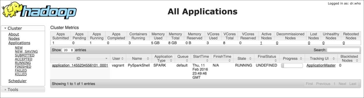
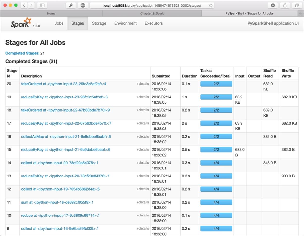
To check the state of the processing, you can use the Spark UI: it's a graphical interface that shows the jobs run by Spark step-by-step. To access the UI, you should first figure out what's the name of the pySpark IPython application, searching in the bash shell where you've launched the notebook by its name (typically, it is in the form application_<number>_<number>), and then point your browser to the page: http://localhost:8088/proxy/application_<number>_<number>
The result is similar to the one in the following image. It contains all the jobs run in spark (as IPython Notebook cells), and you can also visualize the execution plan as a directed acyclic graph (DAG):
Summary
In this chapter, we've introduced some primitives to be able to run distributed jobs on a cluster composed by multiple nodes. We've seen the Hadoop framework and all its components, features, and limitations, and then we illustrated the Spark framework.
In the next chapter, we will dig deep in to Spark, showing how it's possible to do data science in a distributed environment.
All materials on the site are licensed Creative Commons Attribution-Sharealike 3.0 Unported CC BY-SA 3.0 & GNU Free Documentation License (GFDL)
If you are the copyright holder of any material contained on our site and intend to remove it, please contact our site administrator for approval.
© 2016-2026 All site design rights belong to S.Y.A.