Hadoop MapReduce v2 Cookbook, Second Edition (2015)
Chapter 5. Analytics
In this chapter, we will cover the following recipes:
· Simple analytics using MapReduce
· Performing GROUP BY using MapReduce
· Calculating frequency distributions and sorting using MapReduce
· Plotting the Hadoop MapReduce results using gnuplot
· Calculating histograms using MapReduce
· Calculating Scatter plots using MapReduce
· Parsing a complex dataset with Hadoop
· Joining two datasets using MapReduce
Introduction
In this chapter, we will discuss how we can use Hadoop to process a dataset and to understand its basic characteristics. We will cover more complex methods like data mining, classification, clustering, and so on, in later chapters.
This chapter will show how you can calculate basic analytics using a given dataset. For the recipes in this chapter, we will use two datasets:
· The NASA weblog dataset available at http://ita.ee.lbl.gov/html/contrib/NASA-HTTP.html is a real-life dataset collected using the requests received by NASA web servers. You can find a description of the structure of this data at this link. A small extract of this dataset that can be used for testing is available inside the chapter5/resources folder of the code repository.
· List of e-mail archives of Apache Tomcat developers available from http://tomcat.apache.org/mail/dev/. These archives are in the MBOX format.
Note
The contents of this chapter are based on the Chapter 6, Analytics, of the previous edition of this book, Hadoop MapReduce Cookbook. That chapter was contributed by the coauthor Srinath Perera.
Tip
Sample code
The example code files for this book are available in GitHub at https://github.com/thilg/hcb-v2. The chapter5 folder of the code repository contains the sample source code files for this chapter.
Sample codes can be compiled by issuing the gradle build command in the chapter5 folder of the code repository. Project files for Eclipse IDE can be generated by running the gradle eclipse command in the main folder of the code repository. Project files for IntelliJ IDEA IDE can be generated by running the gradle idea command in the main folder of the code repository.
Simple analytics using MapReduce
Aggregate metrics such as mean, max, min, standard deviation, and so on, provide the basic overview of a dataset. You may perform these calculations, either for the whole dataset or to a subset or a sample of the dataset.
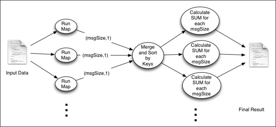
In this recipe, we will use Hadoop MapReduce to calculate the minimum, maximum, and average size of files served from a web server, by processing logs of the web server. The following figure shows the execution flow of this computation:
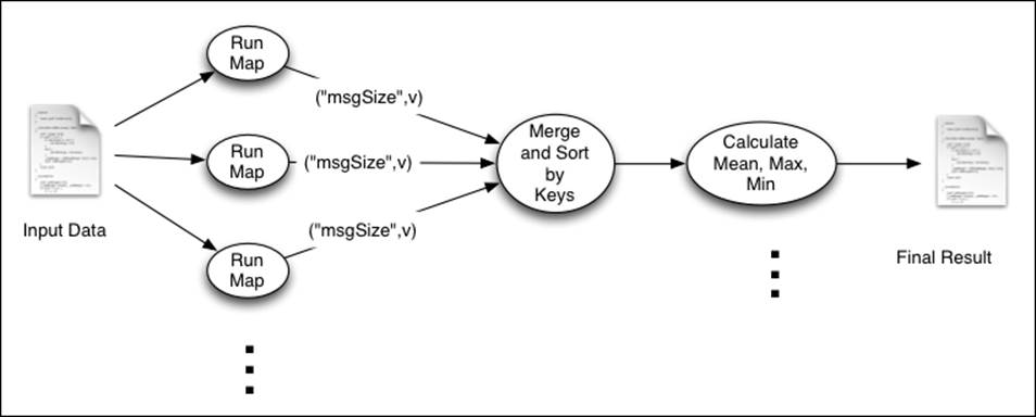
As shown in the figure, the Map function emits the size of the file as the value and the string msgSize as the key. We use a single Reduce task, and all the intermediate key-value pairs will be sent to that Reduce task. Then, the Reduce function calculates theaggregate values using the information emitted by the Map tasks.
Getting ready
This recipe assumes that you have a basic understanding of how the processing of Hadoop MapReduce works. If not, please follow the Writing a WordCount MapReduce application, bundling it, and running it using the Hadoop local mode and Setting up Hadoop YARN in a distributed cluster environment using Hadoop v2 recipes from Chapter 1, Getting Started with Hadoop v2. You need to have a working Hadoop installation as well.
How to do it...
The following steps describe how to use MapReduce to calculate simple aggregate metrics about the weblog dataset:
1. Download the weblog dataset from ftp://ita.ee.lbl.gov/traces/NASA_access_log_Jul95.gz and extract it. Let's call the extracted location as <DATA_DIR>.
2. Upload the extracted data to HDFS by running the following commands:
3. $ hdfs dfs -mkdir data
4. $ hdfs dfs -mkdir data/weblogs
5. $ hdfs dfs –copyFromLocal \
6. <DATA_DIR>/NASA_access_log_Jul95 \
7. data/weblogs
8. Compile the sample source code for this chapter by running the gradle build command from the chapter5 folder of the source repository.
9. Run the MapReduce job by using the following command:
10.$ hadoop jar hcb-c5-samples.jar \
11.chapter5.weblog.MsgSizeAggregateMapReduce \
12.data/weblogs data/msgsize-out
13. Read the results by running the following command:
14.$ hdfs dfs -cat data/msgsize-out/part*
15.….
16.Mean 1150
17.Max 6823936
18.Min 0
How it works...
You can find the source file for this recipe from chapter5/src/chapter5/weblog/MsgSizeAggregateMapReduce.java.
HTTP logs follow a standard pattern as follows. The last token is the size of the web page served:
205.212.115.106 - - [01/Jul/1995:00:00:12 -0400] "GET /shuttle/countdown/countdown.html HTTP/1.0" 200 3985
We will use the Java regular expressions to parse the log lines, and the Pattern.compile() method at the top of the class defines the regular expression. Regular expressions are a very useful tool while writing text-processing Hadoop computations:
public void map(Object key, Text value, Context context) … {
Matcher matcher = httplogPattern.matcher(value.toString());
if (matcher.matches()) {
int size = Integer.parseInt(matcher.group(5));
context.write(new Text("msgSize"), new IntWritable(size));
}
}
Map tasks receive each line in the log file as a different key-value pair. It parses the lines using regular expressions and emits the file size as the value with msgSize as the key.
Then, Hadoop collects all the output key-value pairs from the Map tasks and invokes the Reduce task. Reducer iterates all the values and calculates the minimum, maximum, and mean size of the files served from the web server. It is worth noting that by making the values available as an iterator, Hadoop allows us to process the data without storing them in memory, allowing the Reducers to scale to large datasets. Whenever possible, you should process the reduce function input values without storing them in memory:
public void reduce(Text key, Iterable<IntWritable> values,…{
double total = 0;
int count = 0;
int min = Integer.MAX_VALUE;
int max = 0;
Iterator<IntWritable> iterator = values.iterator();
while (iterator.hasNext()) {
int value = iterator.next().get();
total = total + value;
count++;
if (value < min)
min = value;
if (value > max)
max = value;
}
context.write(new Text("Mean"),
new IntWritable((int) total / count));
context.write(new Text("Max"), new IntWritable(max));
context.write(new Text("Min"), new IntWritable(min));
}
The main() method of the job looks similar to the WordCount example, except for the highlighted lines that have been changed to accommodate the output data types:
job.setOutputKeyClass(Text.class);
job.setOutputValueClass(IntWritable.class);
There's more...
You can learn more about Java regular expressions from the Java tutorial, http://docs.oracle.com/javase/tutorial/essential/regex/.
Performing GROUP BY using MapReduce
This recipe shows how we can use MapReduce to group data into simple groups and calculate metrics for each group. We will use the web server's log dataset for this recipe as well. This computation is similar to the select page, count(*) from weblog_table group by page SQL statement. The following figure shows the execution flow of this computation:
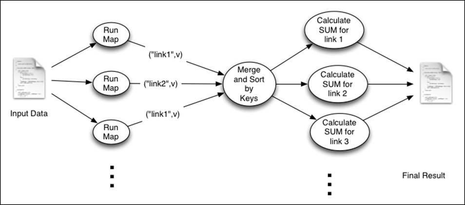
As shown in the figure, the Map tasks emit the requested URL path as the key. Then, Hadoop sorts and groups the intermediate data by the key. All values for a given key will be provided into a single Reduce function invocation, which will count the number of occurrences of that URL path.
Getting ready
This recipe assumes that you have a basic understanding of how Hadoop MapReduce processing works.
How to do it...
The following steps show how we can group web server log data and calculate analytics:
1. Download the weblog dataset from ftp://ita.ee.lbl.gov/traces/NASA_access_log_Jul95.gz and extract it. Let's call the extracted location as <DATA_DIR>
2. Upload the extracted data to HDFS by running the following commands:
3. $ hdfs dfs -mkdir data
4. $ hdfs dfs -mkdir data/weblogs
5. $ hdfs dfs –copyFromLocal \
6. <DATA_DIR>/NASA_access_log_Jul95 \
7. data/weblogs
8. Compile the sample source code for this chapter by running the gradle build command from the chapter5 folder of the source repository.
9. Run the MapReduce job using the following command:
10.$ hadoop jar hcb-c5-samples.jar \
11.chapter5.weblog.HitCountMapReduce \
12.data/weblogs data/hit-count-out
13. Read the results by running the following command:
14.$ hdfs dfs -cat data/hit-count-out/part*
You will see that it will print the results as follows:
/base-ops/procurement/procurement.html 28
/biomed/ 1
/biomed/bibliography/biblio.html 7
/biomed/climate/airqual.html 4
/biomed/climate/climate.html 5
/biomed/climate/gif/f16pcfinmed.gif 4
/biomed/climate/gif/f22pcfinmed.gif 3
/biomed/climate/gif/f23pcfinmed.gif 3
/biomed/climate/gif/ozonehrlyfin.gif 3
How it works...
You can find the source for this recipe from chapter5/src/chapter5/HitCountMapReduce.java.
As described in the earlier recipe, we will use a regular expression to parse the web server logs and to extract the requested URL paths. For example, /shuttle/countdown/countdown.html will get extracted from the following sample log entry:
205.212.115.106 - - [01/Jul/1995:00:00:12 -0400] "GET /shuttle/countdown/countdown.html HTTP/1.0" 200 3985
The following code segment shows the Mapper:
private final static IntWritable one = new IntWritable(1);
private Text word = new Text();
public void map(Object key, Text value, Context context) …… {
Matcher matcher = httplogPattern.matcher(value.toString());
if (matcher.matches()) {
String linkUrl = matcher.group(4);
word.set(linkUrl);
context.write(word, one);
}
}
Map tasks receive each line in the log file as a different key-value pair. Map tasks parse the lines using regular expressions and emit the link as the key and number one as the value.
Then, Hadoop collects all values for different keys (links) and invokes the Reducer once for each link. Then, each Reducer counts the number of hits for each link:
private IntWritable result = new IntWritable();
public void reduce(Text key, Iterable<IntWritable> values,… {
int sum = 0;
for (IntWritable val : values) {
sum += val.get();
}
result.set(sum);
context.write(key, result);
}
Calculating frequency distributions and sorting using MapReduce
Frequency distribution is the number of hits received by each URL sorted in ascending order. We already calculated the number of hits for each URL in the earlier recipe. This recipe will sort that list based on the number of hits.
Getting ready
This recipe assumes that you have a working Hadoop installation. This recipe will use the results from the Performing GROUP BY using MapReduce recipe of this chapter. Follow this recipe if you have not done so already.
How to do it...
The following steps show how to calculate frequency distribution using MapReduce:
1. Run the MapReduce job using the following command. We assume that the data/hit-count-out path contains the output of the HitCountMapReduce computation of the previous recipe:
2. $ bin/hadoop jar hcb-c5-samples.jar \
3. chapter5.weblog.FrequencyDistributionMapReduce \
4. data/hit-count-out data/freq-dist-out
5. Read the results by running the following command:
6. $ hdfs dfs -cat data/freq-dist-out/part*
You will see that it will print the results similar to the following:
/cgi-bin/imagemap/countdown?91,175 12
/cgi-bin/imagemap/countdown?105,143 13
/cgi-bin/imagemap/countdown70?177,284 14
How it works...
The Performing GROUP BY using MapReduce recipe of this chapter calculates the number of hits received by each URL path. MapReduce sorts the Map output's intermediate key-value pairs by their keys before invoking the reduce function. In this recipe, we use this sorting feature to sort the data based on the number of hits.
You can find the source for this recipe from chapter5/src/chapter5/FrequencyDistributionMapReduce.java.
The Map task outputs the number of hits as the key and the URL path as the value:
public void map(Object key, Text value, Context context) …… {
String[] tokens = value.toString().split("\\s");
context.write(new IntWritable(Integer.parseInt(tokens[1])),
new Text(tokens[0]));
}
The Reduce task receives the key-value pairs sorted by the key (number of hits):
public void reduce(IntWritable key, Iterable<Text> values, …… {
Iterator<Text> iterator = values.iterator();
while (iterator.hasNext()) {
context.write(iterator.next(), key);
}
}
We use only a single Reduce task in this computation in order to ensure a global ordering of the results.
There's more...
It's possible to achieve a global ordering even with multiple Reduce tasks, by utilizing the Hadoop TotalOrderPartitioner. Refer to the Hadoop intermediate data partitioning recipe of Chapter 4, Developing Complex Hadoop MapReduce Applications, for more information on the TotalOrderPartitioner.
Plotting the Hadoop MapReduce results using gnuplot
Although Hadoop MapReduce jobs can generate interesting analytics, making sense of those results and getting a detailed understanding about the data often requires us to see the overall trends in the data. The human eye is remarkably good at detecting patterns, and plotting the data often yields a deeper understanding of the data. Therefore, we often plot the results of Hadoop jobs using a plotting program.
This recipe explains how to use gnuplot, which is a free and powerful plotting program used to plot Hadoop results.
Getting ready
This recipe assumes that you have followed the previous recipe, Calculating frequency distributions and sorting using MapReduce. If you have not done this, follow this recipe. Install the gnuplot plotting program by following the instructions inhttp://www.gnuplot.info/.
How to do it...
The following steps show how to plot Hadoop job results using gnuplot:
1. Download the results of the previous recipe to a local computer by running the following command:
2. $ hdfs dfs -copyToLocal data/freq-dist-out/part-r-00000 2.data
3. Copy all the *.plot files from the chapter5/plots folder to the location of the downloaded data.
4. Generate the plot by running the following command:
5. $ gnuplot httpfreqdist.plot
6. It will generate a file called freqdist.png, which will look like the following:
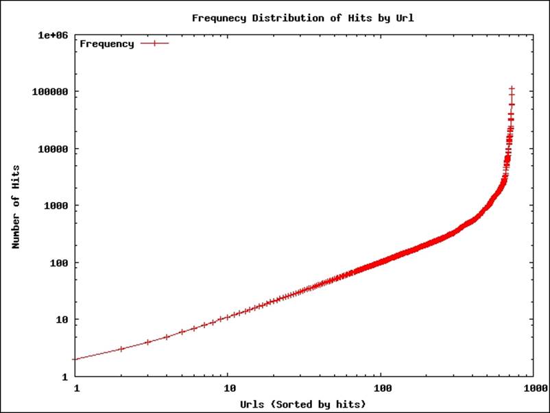
The preceding plot is plotted in log-log scale, and the first part of the distribution follows the zipf (power law) distribution, which is a common distribution seen in the Web. The last few most popular links have much higher rates than expected from a zipf distribution.
Discussion about more details on this distribution is out of the scope of this book. However, this plot demonstrates the kind of insights we can get by plotting the analytical results. In most of the future recipes, we will use gnuplot to plot and analyze the results.
How it works...
The following steps describe how plotting with gnuplot works:
· You can find the source for the gnuplot file from chapter5/plots/httpfreqdist.plot. The source for the plot will look like the following:
· set terminal png
· set output "freqdist.png"
·
· set title "Frequnecy Distribution of Hits by Url";
· set ylabel "Number of Hits";
· set xlabel "Urls (Sorted by hits)";
· set key left top
· set log y
· set log x
·
plot"2.data" using 2 title "Frequency" with linespoints
· Here, the first two lines define the output format. This example uses PNG, but the gnuplot supports many other terminals such as SCREEN, PDF, EPS, and so on.
· The next four lines define the axis labels and the title.
· The next two lines define the scale of each axis, and this plot uses log scale for both.
· The last line defines the plot. Here, it is asking gnuplot to read the data from the 2.data file, and use the data in the second column of the file via using 2 and to plot it using lines. Columns must be separated by whitespaces.
· Here, if you want to plot one column against another, for example, data from column 1 against column 2, you should write using 1:2 instead of using 2.
There's more...
You can learn more about gnuplot from http://www.gnuplot.info/.
Calculating histograms using MapReduce
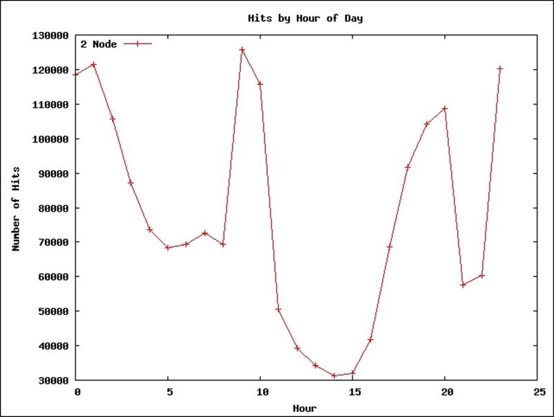
Another interesting view of a dataset is a histogram. A histogram makes sense only under a continuous dimension (for example, accessed time and file size). It groups the number of occurrences of an event into several groups in the dimension. For example, in this recipe, if we take the accessed time as the dimension, then we will group the accessed time by the hour.
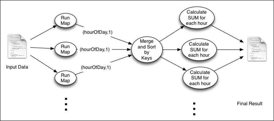
The following figure shows the execution summary of this computation. The Mapper emits the hour of the access as the key and 1 as the value. Then, each reduce function invocation receives all the occurrences of a certain hour of the day, and it calculates the total number of occurrences for that hour of the day.
Getting ready
This recipe assumes that you have a working Hadoop installation. Install gnuplot.
How to do it...
The following steps show how to calculate and plot a histogram:
1. Download the weblog dataset from ftp://ita.ee.lbl.gov/traces/NASA_access_log_Jul95.gz and extract it.
2. Upload the extracted data to HDFS by running the following commands:
3. $ hdfs dfs -mkdir data
4. $ hdfs dfs -mkdir data/weblogs
5. $ hdfs dfs –copyFromLocal \
6. <DATA_DIR>/NASA_access_log_Jul95 \
7. data/weblogs
8. Compile the sample source code for this chapter by running the gradle build command from the chapter5 folder of the source repository.
9. Run the MapReduce job using the following command:
10.$ hadoop jar hcb-c5-samples.jar \
11.chapter5.weblog.HistogramGenerationMapReduce \
12.data/weblogs data/histogram-out
13. Inspect the results by running the following command:
14.$ hdfs dfs -cat data/histogram-out/part*
15. Download the results to a local computer by running the following command:
16.$ hdfs dfs -copyToLocal data/histogram-out/part-r-00000 3.data
17. Copy all the *.plot files from the chapter5/plots folder to the location of the downloaded data.
18. Generate the plot by running the following command:
19.$gnuplot httphistbyhour.plot
20. It will generate a file called hitsbyHour.png, which will look like the following:
How it works...
You can find the source code for this recipe from chapter5/src/chapter5/weblog/HistogramGenerationMapReduce.java. Similar to the earlier recipes of this chapter, we use a regular expression to parse the log file and extract the access time from the log files.
The following code segment shows the map function:
public void map(Object key, Text value, Context context) … {
try {
Matcher matcher = httplogPattern.matcher(value.toString());
if (matcher.matches()) {
String timeAsStr = matcher.group(2);
Date time = dateFormatter.parse(timeAsStr);
Calendar calendar = GregorianCalendar.getInstance();
calendar.setTime(time);
int hour = calendar.get(Calendar.HOUR_OF_DAY);
context.write(new IntWritable(hour), one);
}
} ……
}
The map function extracts the access time for each web page access and extracts the hour of the day from the access time. It emits the hour of the day as the key and one as the value.
Then, Hadoop collects all key-value pairs, sorts them, and then invokes the Reduce function once for each key. Reduce tasks calculate the total page views for each hour:
public void reduce(IntWritable key, Iterable<IntWritable> values,..{
int sum = 0;
for (IntWritable val : values) {
sum += val.get();
}
context.write(key, new IntWritable(sum));
}
Calculating Scatter plots using MapReduce
Another useful tool while analyzing data is a Scatter plot, which can be used to find the relationship between two measurements (dimensions). It plots the two dimensions against each other.
For example, this recipe analyzes the data to find the relationship between the size of the web pages and the number of hits received by the web page.
The following image shows the execution summary of this computation. Here, the map function calculates and emits the message size (rounded to 1024 bytes) as the key and one as the value. Then, the Reducer calculates the number of occurrences for each message size:
Getting ready
This recipe assumes that you have a working Hadoop installation. Install gnuplot.
How to do it...
The following steps show how to use MapReduce to calculate the correlation between two datasets:
1. Download the weblog dataset from ftp://ita.ee.lbl.gov/traces/NASA_access_log_Jul95.gz and extract it.
2. Upload the extracted data to HDFS by running the following commands:
3. $ hdfs dfs -mkdir data
4. $ hdfs dfs -mkdir data/weblogs
5. $ hdfs dfs –copyFromLocal \
6. <DATA_DIR>/NASA_access_log_Jul95 \
7. data/weblogs
8. Compile the sample source code for this chapter by running the gradle build command from the chapter5 folder of the source repository.
9. Run the MapReduce job using the following command:
10.$ hadoop jar hcb-c5-samples.jar \
11.chapter5.weblog.MsgSizeScatterMapReduce \
12.data/weblogs data/scatter-out
13. Inspect the results by running the following command:
14.$ hdfs dfs -cat data/scatter-out/part*
15. Download the results of the previous recipe to the local computer by running the following command from HADOOP_HOME:
16.$ hdfs dfs –copyToLocal data/scatter-out/part-r-00000 5.data
17. Copy all the *.plot files from the chapter5/plots folder to the location of the downloaded data.
18. Generate the plot by running the following command:
19.$ gnuplot httphitsvsmsgsize.plot
20. It will generate a file called hitsbymsgSize.png, which will look like the following image:
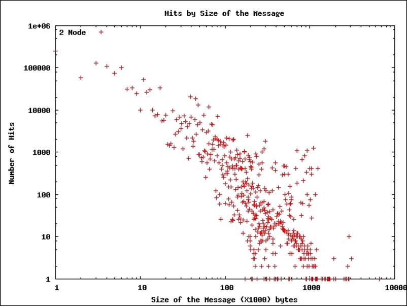
The plot shows a negative correlation between the number of hits and the size of the messages in the log scales.
How it works...
You can find the source for the recipe from chapter5/src/chapter5/MsgSizeScatterMapReduce.java.
The following code segment shows the map function:
public void map(Object key, Text value, Context context) …… {
Matcher matcher = httplogPattern.matcher(value.toString());
if (matcher.matches()) {
int size = Integer.parseInt(matcher.group(5));
context.write(new IntWritable(size / 1024), one);
}
}
Map tasks parse the log entries and emit the file size in kilobytes as the key and one as the value.
Each Reducer walks through the values and calculates the count of page accesses for each file size:
public void reduce(IntWritable key, Iterable<IntWritable> values,……{
int sum = 0;
for (IntWritable val : values) {
sum += val.get();
}
context.write(key, new IntWritable(sum));
}
Parsing a complex dataset with Hadoop
The datasets we used so far contained a data item in a single line, making it possible for us to use Hadoop default parsing support to parse those datasets. However, some datasets have more complex formats, where a single data item may span multiple lines. In this recipe, we will analyze mailing list archives of Tomcat developers. In the archive, each e-mail consists of multiple lines of the archive file. Therefore, we will write a custom Hadoop InputFormat to process the e-mail archive.
This recipe parses the complex e-mail list archives, and finds the owner (the person who started the thread) and the number of replies received by each e-mail thread.
The following figure shows the execution summary of this computation. The Map function emits the subject of the mail as the key, and the sender's e-mail address combined with the date as the value. Then, Hadoop groups the data by the e-mail subject and sends all the data related to that thread to the same Reducer.
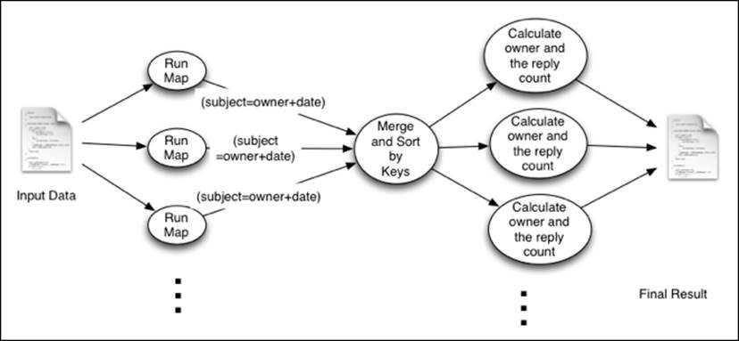
Then, the Reduce tasks identify the creator of each e-mail thread and the number of replies received by each thread.
Getting ready
This recipe assumes that you have a working Hadoop installation.
How to do it...
The following steps describe how to parse the Tomcat e-mail list dataset that has complex data format using Hadoop by writing an input formatter:
1. Download and extract the Apache Tomcat developer list e-mail archives for the year 2012 from http://tomcat.apache.org/mail/dev/. We call the destination folder as DATA_DIR.
2. Upload the extracted data to HDFS by running the following commands:
3. $ hdfs dfs -mkdir data
4. $ hdfs dfs -mkdir data/mbox
5. $ hdfs dfs –copyFromLocal \
6. <DATA_DIR>/* \
7. data/mbox
8. Compile the sample source code for this chapter by running the gradle build command from the chapter5 folder of the source repository.
9. Run the MapReduce job using the following command:
10.$ hadoop jar hcb-c5-samples.jar \
11.chapter5.mbox.CountReceivedRepliesMapReduce \
12.data/mbox data/count-replies-out
13. Inspect the results by running the following command:
14.$ hdfs dfs -cat data/count-replies-out/part*
How it works...
As explained before, this dataset has data items that span multiple lines. Therefore, we have to write a custom InputFormat and a custom RecordReader to parse the data. Source code files for this recipe are the CountReceivedRepliesMapReduce.java,MBoxFileInputFormat.java, and MBoxFileReader.java files in the chapter5/src/chapter5/mbox directory of the source code archive.
We add the new InputFormat to the Hadoop job via the Hadoop driver program as highlighted in the following code snippet:
Job job = Job.getInstance(getConf(), "MLReceiveReplyProcessor");
job.setJarByClass(CountReceivedRepliesMapReduce.class);
job.setMapperClass(AMapper.class);
job.setReducerClass(AReducer.class);
job.setNumReduceTasks(numReduce);
job.setOutputKeyClass(Text.class);
job.setOutputValueClass(Text.class);
job.setInputFormatClass(MBoxFileInputFormat.class);
FileInputFormat.setInputPaths(job, new Path(inputPath));
FileOutputFormat.setOutputPath(job, new Path(outputPath));
int exitStatus = job.waitForCompletion(true) ? 0 : 1;
As shown in the following code, the new formatter creates a RecordReader, which is used by Hadoop to read the key-value pair input to the Map tasks:
public class MboxFileFormat extends FileInputFormat<Text, Text>{
private MBoxFileReaderboxFileReader = null;
public RecordReader<Text, Text> createRecordReader(
InputSplit inputSplit, TaskAttemptContext attempt) …{
fileReader = new MBoxFileReader();
fileReader.initialize(inputSplit, attempt);
return fileReader;
}
}
The following code snippets show the functionality of the RecordReader:
public class MBoxFileReader extends RecordReader<Text, Text> {
public void initialize(InputSplitinputSplit, … {
Path path = ((FileSplit) inputSplit).getPath();
FileSystem fs = FileSystem.get(attempt.getConfiguration());
FSDataInputStream fsStream = fs.open(path);
reader = new BufferedReader(new InputStreamReader(fsStream));
}
public Boolean nextKeyValue() ……{
if (email == null) {
return false;
}
count++;
while ((line = reader.readLine()) != null) {
Matcher matcher = pattern1.matcher(line);
if (!matcher.matches()) {
email.append(line).append("\n");
} else {
parseEmail(email.toString());
email = new StringBuffer();
email.append(line).append("\n");
return true;
}
}
parseEmail(email.toString());
email = null;
return true;
}
………
The nextKeyValue() method of the RecordReader parses the file, and generates key-value pairs for the consumption by the Map tasks. Each value has the from, subject, and time of each e-mail separated by a # character.
The following code snippet shows the Map task source code:
public void map(Object key, Text value, Context context) …… {
String[] tokens = value.toString().split("#");
String from = tokens[0];
String subject = tokens[1];
String date = tokens[2].replaceAll(",", "");
subject = subject.replaceAll("Re:", "");
context.write(new Text(subject), new Text(date + "#" + from));
}
The Map task receives each e-mail in the archive files as a separate key-value pair. It parses the lines by breaking it by the #, and emits the subject as the key, and time and from as the value.
Then, Hadoop collects all key-value pairs, sorts them, and then invokes the Reducer once for each key. Since we use the e-mail subject as the key, each Reduce function invocation will receive all the information about a single e-mail thread. Then, the Reduce function will analyze all the e-mails of a thread and find out who sent the first e-mail and how many replies have been received by each e-mail thread as follows:
public void reduce(Text key, Iterable<Text> values, …{
TreeMap<Long, String>replyData = new TreeMap<Long, String>();
for (Text val : values) {
String[] tokens = val.toString().split("#");
if(tokens.length != 2)
throw new IOException("Unexpected token "+ val.toString());
String from = tokens[1];
Date date = dateFormatter.parse(tokens[0]);
replyData.put(date.getTime(), from);
}
String owner = replyData.get(replyData.firstKey());
Int replyCount = replyData.size();
Int selfReplies = 0;
for(String from: replyData.values()){
if(owner.equals(from)){
selfReplies++;
}
}
replyCount = replyCount - selfReplies;
context.write(new Text(owner),
new Text(replyCount+"#" + selfReplies));
}
There's more...
Refer to the Adding support for new input data formats – implementing a custom InputFormat recipe of Chapter 4, Developing Complex Hadoop MapReduce Applications, for more information on implementing custom InputFormats.
Joining two datasets using MapReduce
As we have already observed, Hadoop is very good at reading through a dataset and calculating the analytics. However, we will often have to merge two datasets to analyze the data. This recipe will explain how to join two datasets using Hadoop.
As an example, this recipe will use the Tomcat developer archives dataset. A common belief among the open source community is that the more a developer is involved with the community (for example, by replying to e-mail threads in the project's mailing lists and helping others and so on), the more quickly they will receive responses to their queries. In this recipe, we will test this hypothesis using the Tomcat developer mailing list.
To test this hypothesis, we will run the MapReduce jobs as explained in the following figure:
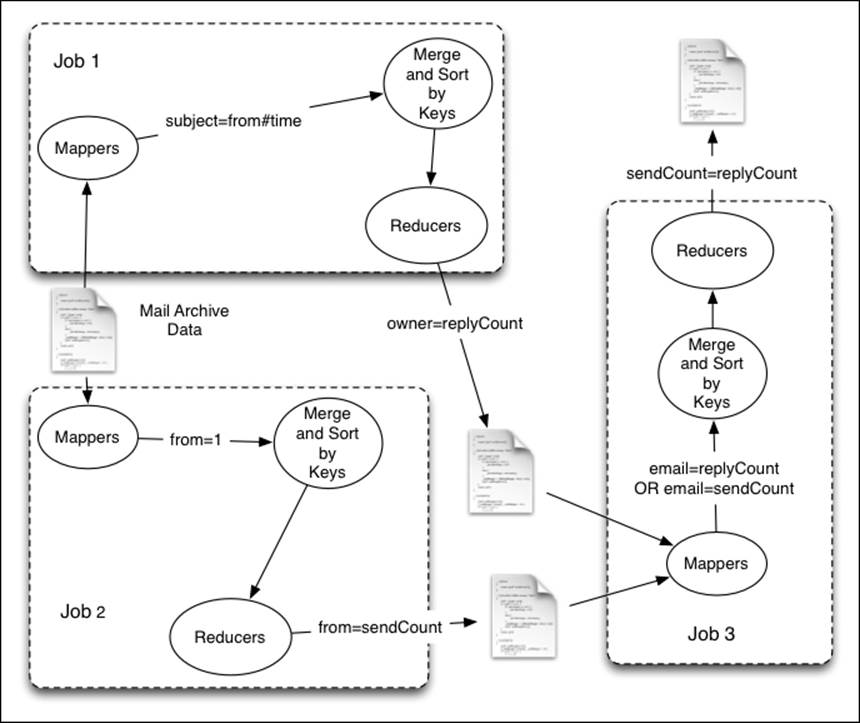
We will use the MBOX-formatted e-mail archives and use the custom InputFormat and RecordReader explained in the earlier recipe to parse them. Map tasks will receive the sender of the e-mail (from), the e-mail subject, and the time the e-mail was sent, as inputs.
1. In the first job, the map function will emit the subject as the key, and the sender's e-mail address and time as the value. Then, the Reducer step will receive all the values with the same subject and it will output the subject as the key, and the owner and reply count as the value. We executed this job in the previous recipe.
2. In the second job, the map function emits the sender's e-mail address as the key and one as the value. Then, the Reducer step will receive all the e-mails sent from the same address to the same Reducer. Using this data, each Reducer will emit the e-mail address as the key and the number of e-mails sent from that e-mail address as the value.
3. Finally, the third job reads both the outputs from the preceding two jobs, joins the results, and emits the number of e-mails sent by each e-mail address and the number of replies received by each e-mail address as the output.
Getting ready
This recipe assumes that you have a working Hadoop installation. Follow the Parsing a complex dataset with Hadoop recipe. We will use the input data and the output data of that recipe in the following steps.
How to do it...
The following steps show how to use MapReduce to join two datasets:
1. Run the CountReceivedRepliesMapReduce computation by following the Parsing a complex dataset with Hadoop recipe.
2. Run the second MapReduce job using the following command:
3. $ hadoop jar hcb-c5-samples.jar \
4. chapter5.mbox.CountSentRepliesMapReduce \
5. data/mbox data/count-emails-out
6. Inspect the results by using the following command:
7. $ hdfs dfs -cat data/count-emails-out/part*
8. Create a new folder join-input and copy both the results from the earlier jobs to that folder in HDFS:
9. $ hdfs dfs -mkdir data/join-input
10.$ hdfs dfs -cp \
11.data/count-replies-out/part-r-00000 \
12.data/join-input/1.data
13.$ hdfs dfs -cp \
14.data/count-emails-out/part-r-00000 \
15.data/join-input/2.data
16. Run the third MapReduce job using the following command:
17.$ hadoop jar hcb-c5-samples.jar \
18.chapter5.mbox.JoinSentReceivedReplies \
19.data/join-input data/join-out
20. Download the results of step 5 to the local computer by running the following command:
21.$ hdfs dfs -copyToLocal data/join-out/part-r-00000 8.data
22. Copy all the *.plot files from the chapter5/plots folder to the location of the downloaded data.
23. Generate the plot by running the following command:
24.$ gnuplot sendvsreceive.plot
25. It will generate a file called sendreceive.png, which will look like the following:
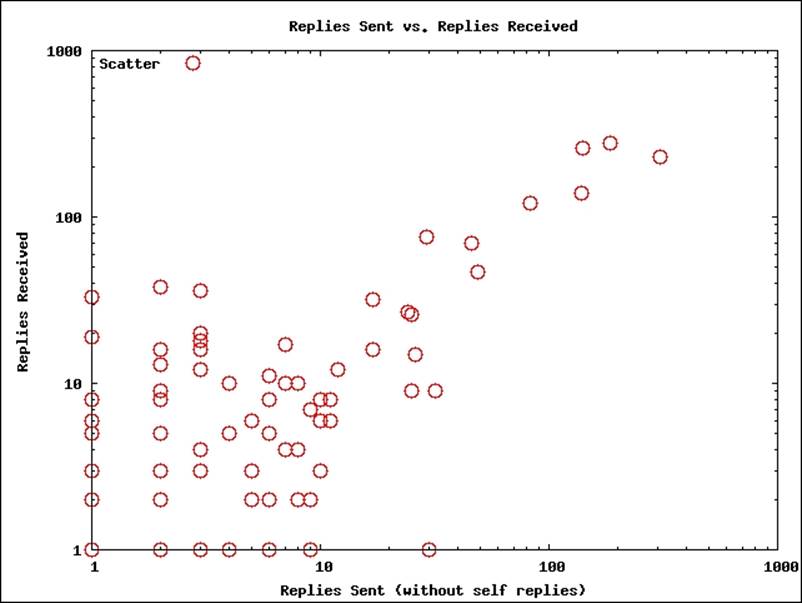
The graph confirms our hypothesis, and like before, the data approximately follows a power law distribution.
How it works...
You can find the source code for this recipe from chapter5/src/chapter5/mbox/CountSentRepliesMapReduce.java and chapter5/src/chapter5/mbox/JoinSentReceivedReplies.java. We have already discussed the first job in the earlier recipe.
The following code snippet shows the map function for the second job. It receives the sender's e-mail, subject, and time separated by # as the input, which parses the input and outputs the sender's e-mail as the key, and the time the e-mail was sent as the value:
public void map(Object key, Text value, Context context) ……{
String[] tokens = value.toString().split("#");
String from = tokens[0];
String date = tokens[2];
context.write(new Text(from), new Text(date));
}
The following code snippet shows the reduce function for the second job. Each reduce function invocation receives the time of all the e-mails sent by one sender. The Reducer counts the number of replies sent by each sender, and outputs the sender's name as the key, and the number of replies sent as the value:
public void reduce(Text key, Iterable<Text> values, ……{
int sum = 0;
for (Text val : values) {
sum = sum +1;
}
context.write(key, new IntWritable(sum));
}
The following code snippet shows the map function for the third job. It reads the outputs of the first and second jobs, and outputs them as the key-value pairs:
public void map(Object key, Text value, …… {
String[] tokens = value.toString().split("\\s");
String from = tokens[0];
String replyData = tokens[1];
context.write(new Text(from), new Text(replyData));
}
The following code snippet shows the reduce function for the third job. Since both the outputs of the first and the second job have the same key, the number of replies sent and the number of replies received by a given user will be processed by the same Reducer. The reduce function removes self-replies and outputs the number of replies sent and the number of replies received as the key and value, thus joining the two datasets:
public void reduce(Text key, Iterable<Text> values, …… {
StringBuffer buf = new StringBuffer("[");
try {
int sendReplyCount = 0;
int receiveReplyCount = 0;
for (Text val : values) {
String strVal = val.toString();
if(strVal.contains("#")){
String[] tokens = strVal.split("#");
int repliesOnThisThread =Integer.parseInt(tokens[0]);
int selfRepliesOnThisThread = Integer.parseInt(tokens[1]);
receiveReplyCount = receiveReplyCount + repliesOnThisThread;
sendReplyCount = sendReplyCount–selfRepliesOnThisThread;
}else{
sendReplyCount = sendReplyCount + Integer.parseInt(strVal);
}
}
context.write(new IntWritable(sendReplyCount),
new IntWritable(receiveReplyCount));
buf.append("]");
} …
}
The final job is an example of using the MapReduce to join two datasets. The idea is to send all the values that need to be joined under the same key to the same Reducer, and join the data there.
All materials on the site are licensed Creative Commons Attribution-Sharealike 3.0 Unported CC BY-SA 3.0 & GNU Free Documentation License (GFDL)
If you are the copyright holder of any material contained on our site and intend to remove it, please contact our site administrator for approval.
© 2016-2026 All site design rights belong to S.Y.A.