Minitab Cookbook (2014)

Chapter 11. Macro Writing

In this chapter, we will cover the following recipes:

· Exec macros to repeat simple commands

· Building a Global macro to create a custom graph layout

· Obtaining input from the session window with a Global macro

· Creating a Local macro

· Local macros with subcommands, submacros, and control statements

Introduction

Minitab does have a macro language that can be used to automate simple tasks or run more sophisticated functions. Here, we will explore the three different types of macro in Minitab. The recipes follow a set of commands that are used to create a panel of charts. In each recipe, we will build on the previous example until we get to the final, complicated, but sophisticated, Local macro. This will show you the differences between the macro types and why you may want to use one type over another.

The macro language in Minitab shares a lot of similarities with Fortran, and here Minitab shows its pedigree. The first version was written in Fortran at Penn State University in 1972!

Minitab also has an Application Programming Interface (API) that can be programmed to use Visual Basic and other languages. Anyone looking to use the API will find Minitab type libraries and references that they can use as part of the installation of Minitab. Programming the API, though, goes beyond the scope of this book.

What is the difference between the macro types?

Exec macros are just the command language in a text file. When Minitab reads this command language, it will run the steps in order. You cannot use any control statements, such as the IF statements or DO loops within an Exec. Execs, though, can be quite useful as a very quick way of repeating the same steps on new data. They work directly in the worksheet in Minitab. They use the *.MTB file extension.

Global macros are one step more advanced than Execs. They allow for the use of control statements. Like Exec files, they work directly from the worksheet in Minitab. Both Execs and Global macros will refer to columns in the worksheet either by column number, such as C10, or by a column name. Those columns must exist in the worksheet in the same format for the macros to run properly. They use the *.MAC file extension.

Local macros, when called, are told which columns, constants, or matrices to use, and they take this information into the macro. We have to specify the data types for columns and constants within these macros as we use them. Local macros are more typical of a programming language. They are more flexible to use, as by calling the macro, we identify which data to use from the worksheet. They can work on any worksheet and are not limited to using the same column, either by name or number. The *.MAC file extension is used for Local macros as well.

Furthermore, we can call macros from within other macros. These can be held in the same macro file or can call external macro files. In calling other macros, we have to be aware of which macro types can call other macro types. The following table can be used to see how macros can call other macros:

The rows show you the macro that is running, and the columns show you the macro being called.

Useful information for writing macros

The history folder in Minitab is an invaluable help in writing macros. Most of the commands that we use in the menus have text commands associated with them; as we run the commands in the Stat or Graph menus, this text is stored in the history folder.

We could, however, type the text commands directly into Minitab to create charts or studies without the use of the menus. For instance, the PLOT C1*C2 command will create a scatterplot of column 1 and column 2.

These commands can be entered either into the session window or the command-line editor. To enter commands in the session window, we need to enable the use of the command language. To achieve this, select the session window, go to the Editor menu, and select Enable Commands. This should switch on a MTB > command prompt in the session window. Commands can be entered after this prompt and you can then click on enter to run them. The command language for the session window is disabled by default, but we can change this within options and the section for the session window.

The command-line editor can be accessed from the Edit menu or by pressing Ctrl + L. The benefit of the command-line editor is that it remembers the previous commands that were used. We can also type several lines into the command-line editor and run them in one step by clicking on Submit Commands. This can be useful to test small sections of code.

Macros can be written in any text editor. Notepad is used here as it is freely available and offers a simple interface. The macros must be saved correctly though, and when using Save As… in Notepad, it will add a *.TXT file extension to every file unless we specify that the file type should be save as All files.

Notepad does not allow users to highlight syntax. To see the structure of the macro, spaces are used, which helps follow code, subcommands, and sections for If and Do loops. Other text editors will allow us to color the code.

When writing a macro, it is possible to use Minitab to generate as much of the syntax as possible. By running the command from the menus, we can go to the history folder and take the code from there.

The help files within Minitab also contain a great resource for most of the commands that we can use in macros. From the main help screen, we should select macros from the references section. Then, from the top of the Using Macros help page, select the See also link. The Alphabetical command list option is a great location to read up on most of Minitab's commands.

Preparing to run macros

To run Exec files, navigate to File | Other Files | Run an Exec…; or, we could enter the Execute command with the path and the file name to run the Exec. This is shown as follows:

Execute "C:\Users\...\Macros\Report.mtb" 1.

Macros are run by entering a % symbol in front of the path and filename, as shown in the following command:

%"C:\Users\...\Macros\montecarlo.mac"

This can be simplified by specifying the folder where macros are saved in Options…. Under the Tools menu, select Options…. The Macro location: section can be used to point to macros.

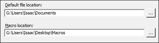
Macros saved in the macro location folder only need to be referred to with % and the filename. The recipes here will assume that we have set the macro location and that our macros are saved within this location.

Debugging

Many times, a macro will fail to run because of a small syntax error. Typically, a missing ; symbol or the incorrect use of " instead of ' can cause all sorts of problems. To help with debugging, the following commands prove invaluable:

· PLUG: This command is used to tell a macro to run and ignore errors in the code that would cause it to not run. It will run through the macro until it hits a problem.

· NOPLUG: This command turns PLUG off.

· ECHO: This command is used to print each line into the session window while it is run.

· NOECHO: This command turns Echo off.

· NOTE: This command is written after a note is printed in the session window. Using NOTE and a number, for instance, can tell where you have reached in the macro.

· #: This is used to enter notes into the macro. Anything written after # will not be read.

Exec macros to repeat simple commands

Exec macros are the simplest form of macros that can be written in Minitab. They are only session commands that are saved in a text file. Exec files must use the *.MTB file extension.

Here, we will use data in the Macro data.mtw worksheet to create an Exec file to automate the running of several charts. If we regularly work from a set of data in the same format each week or each month, then we can use a simple Exec such as this one to run all the commands that we would use in the menus.

The Exec file will generate probability, histogram, and time series plots and will then run 1 sample t-test and a 1 Variance test on the data.

We will run the tools from the menus in Minitab in sequence, before using the commands from the history folder to save them as an Exec file.

Getting ready

Open the Macro Data.MTW worksheet by going to the File menu and selecting Open worksheet….

How to do it…

The following instructions will use the history folder to build a simple Exec file to generate a series of graphs:

1. Go to the Graph menu and select Probability Plot….

2. Select the Single plot.

3. Enter Data in the Graph variables: section.

4. Click on OK.

5. Go to the Graph menu and select Time Series Plot….

6. Select the Simple chart.

7. Enter Data in the Series: section.

8. Click on OK.

9. Go to the Graph menu and select Histogram….

10. Select the With Fit and Groups option.

11. Enter Data in the Graph Variables: section.

12. Click on OK.

13. Navigate to Stat | Basic statistics and select 1-sample t-test.

14. Enter Data in the One or more samples, each in a column: section.

15. Check the option for Perform hypothesis test and enter 10 for Hypothesized mean:.

16. Click on OK.

17. Navigate to Stat | Basic statistics and select 1 Variance….

18. Enter Data in the One or more samples, each in a column: section.

19. Check the option for Perform hypothesis test.

20. Enter 2 in Value:.

21. Click on OK.

22. Go to the history folder, which is the yellow icon on the project manager toolbar, as shown in the following screenshot:

23. Highlight the commands from PPlot to the end of the OneVariance test, as shown in the following screenshot:

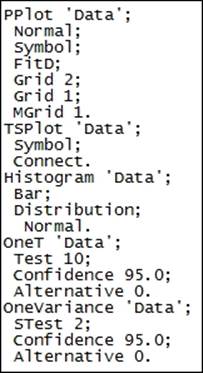
24. Right-click on the selected commands and go to Save As….

25. Name the file as Report and choose the Save as type: option as Exec Files – ANSI (*.MTB).

26. Navigate to the macro directory and click on Save.

27. To run the macro, go to the File menu and select Other Files and Run an Exec….

28. Click on Select File.

29. Navigate to the macro folder and select the Report.mtb file.

30. Click on Open to run the Exec file.

How it works…

The Exec file is only a text file and can be edited by opening it in Notepad or any other text editor. Exec files can be created by writing or pasting the commands directly into Notepad as well as saving them directly from the history folder. The ANSI denomination on the file is short for American National Standards Institute. Typically, saving the Exec file as an ANSI formatted text should avoid any issues with compatibility.

Minitab will run commands in the order that they are saved in the Exec file. In this manner, they can be created very quickly and simply by using the menus to generate the desired output and then selecting the commands from the history folder.

After following the previous steps, the Exec will always look for a column labeled Data to generate the output. If a worksheet does not contain a column of this name, the Exec file will not work. As an alternative, we can use the column references, C, and the column number to point to a specific column.

The Number of times to execute: field allows an iterative Exec to be run. This can be useful as a simple way to run a simulation. If we want to estimate a parameter with a Monte Carlo simulation, we can use the number of times the file is executed as a way of taking multiple sample points.

There's more…

There are several commands that can be added to help an output in Minitab. The XWORD command will output the charts and session window to Word, and XPPOINT will output to PowerPoint. Adding either of these to the end of the Exec file will send everything in the session window and all charts directly into either application.

Graphs can be sent into the Report pad within Minitab by use of the GMANAGER command with an APPEND subcommand. This works only for graphs in the project and not for results in the session window.

We can use the Exec file to split the worksheet, subset the worksheet, and more. These data tools generate new worksheets. The macro will continue running within the active worksheet after splitting or subsetting it. Should we need to swap to a different worksheet, then the Worksheet command used with the worksheet name can be used to swap between worksheets in a project. Constants, columns, and matrices remain unique to a worksheet; storing a constant in one worksheet will not be available in a second worksheet.

See also

· The Using probability plots to check the distribution of two sets of data recipe in Chapter 2, Tables and Graphs

· The Creating a time series plot recipe in Chapter 2, Tables and Graphs

· The Comparing the population mean to a target with a 1-Sample t-test recipe in Chapter 3, Basic Statistical Tools

Building a Global macro to create a custom graph layout

In this recipe, we will generate a custom layout of graphs. We will convert the previous recipe's Exec file into a Global macro and place all the charts on one page.

Global macros are similar to Exec files in that they look at the worksheet for the datasets. Like Exec files, they will use column names or references to identify the data to be used.

A benefit of Global macros over Execs is the ability to specify control statements such as DO and IF.

We will edit the report.MTB file generated in the previous example to place the histogram, probability, and time series plot into a single graphical layout. We will also edit the time series chart, add specification limits, and adjust the color and type of the reference line.

Getting ready

Open the Macro Data.MTW worksheet in Minitab and open the Exec file created in the previous recipe or the catch-up report.MTB file in Notepad.

How to do it…

The following steps will convert the Exec file created in the previous recipe into a Global macro. We will also place the graphs into a single graph page:

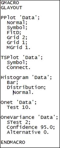
1. In the Report.MTB Exec file, add GMACRO to the top line in Notepad and as a second line, add GLAYOUT.

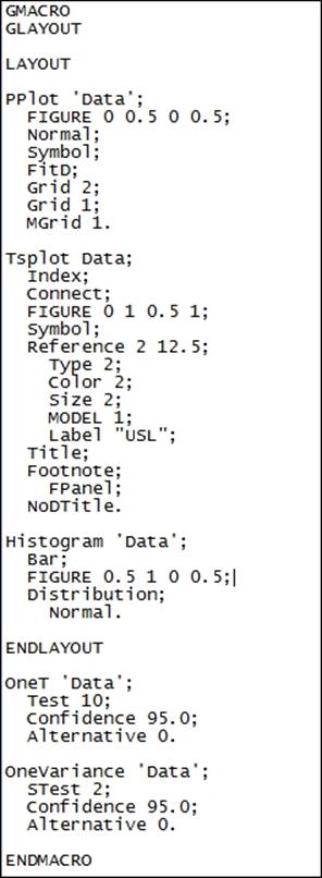
2. On the last line, add ENDMACRO so the macro looks like the following screenshot:

3. Save the file in the macro directory with the name Glayout.mac.

4. Press Ctrl + L to bring up the command-line editor. Enter the %glayout command and click on the Submit command.

Note

It is good practice to test macros as they are being worked on to see if they still run. If the macro fails to run, check if the macro directory is specified correctly. Also check if there is a column named Data in the worksheet.

5. Select the time series plot that the macro generated and right-click on the chart. From the right-click menu, go to Add and then select Add Reference Lines….

6. In the Show reference lines at Y values: section, enter 12.5 and click on OK.

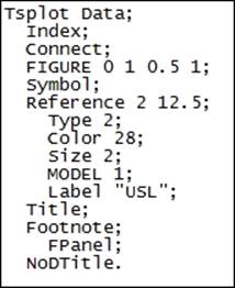
7. Double-click on the reference line that is generated and change the line to a Custom type. Select a dashed line, a red color, and make the size of the line 2.

8. Click on OK.

9. Double-click on the label of 12.5 on the reference line.

10. Change the Text: value to USL and click on OK.

11. Go to the Editor menu and select the Copy Command Language option.

The Editor menu is context specific and will only show options that are relevant to the selected window. If the Copy Command Language option is not available, left-click on the chart and go back to the Editor menu.

Return to the macro in Notepad.

Delete the text for the time series plot. This should start with TSPlot Data; and continue to the line Connect;.

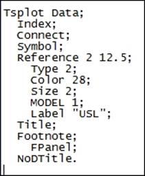
Paste the copied commands into the section where the old TSPlot command was. The command for the time series plot should now look like the following screenshot:

12. To start a graph layout, enter Layout before the PPlot probability plot command.

13. To finish the graph layout, enter Endlayout after the Histogram command.

14. The graphs will need to be positioned on the layout page. For the PPlot command, add the Figure 0 0.5 0 0.5; line as a subcommand.

15. For a histogram, add the Figure 0.5 1 0 0.5; command-line.

16. For the time series plot, add Figure 0 1 0.5 1; to ensure that the macro looks similar to the following screenshot:

17. Save the macro and test it to see if it works by going back to Minitab.

18. Press Ctrl + L to open the command-line editor and enter %glayout and click on Submit Commands to run the macro.

How it works…

Global macros use the GMacro header to identify whether they are Global macros. They also require the second line to be a name for the macro. Finally, macros must finish with the EndMacro command.

The macro's name is relevant only if several macros are used in the same file; for an example, see the Local macros with subcommands, submacros, and control statements recipe. The name of the macro is used to call that macro. To invoke a macro saved in the same file, we would use the Call Macroname command. If we are invoking a macro saved as a separate file, we would use the %Macroname command.

The copy command language functionality is an excellent method to edit charts visually and then obtain the text of those commands to use them in a macro.

Copy command language is a function that works only for the updating graphs in Minitab. This includes only the charts that we create from the Graph menu and the control charts. Most graphs created from the Stat menu do not update and have fewer subcommands. The Figure subcommand that we have used here, for instance, is only available for updating charts.

For a list of the subcommands that can be used by charts in either the Stat or the Graph menu, see the Help section and the Alphabetical command list, as discussed in the Introduction section.

The command and subcommand structure is defined by the use of full stops and semicolons. A full stop is used to end a command and a semicolon continues the command on the next line with a new subcommand. Any command that is only run on one line does not need the full stop to end the command. The following is an example of such a command line:

Plot C1*C2

If we were to include a regression fit to the scatterplot, the command would then need to be as follows:

Plot C1*C2;

Regress.

The Figure commands in this example used a semicolon to continue the subcommands. If the Figure commands are the last line of the command, they should be followed by a full stop.

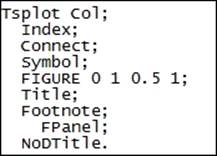
Subcommands do not have any requirement to be placed in a specific order. Figure could be entered as the first or the last subcommand, or anywhere in between. Although, it must be noted that subcommands of subcommands must be included in the relevant section, as shown in the following screenshot:

The reference subcommand for the time series plot places the reference line on the y axis, and the subcommands, such as Type, Color, and Size, all detail properties of that line. If Type does not follow the reference section, the Tsplot command will generate an error.

In the preceding code, Index, Connect, Symbol, and Reference could be entered in any order. Type, Color, Size, Model, and Label refer to the Reference subcommand and must appear with a reference.

The Layout command has two parts. Layout starts a graphical layout; any new chart that is created will be held waiting until the Endlayout command is given. All graphs created between those two commands are placed on the same page. If we do not position the graphs with the Figure subcommand, they would all be placed on top of each other. The Figure command defines the page position in the following way:

Figure X1 X2 Y1 Y2

Here, 0 0 0 0 defines the bottom-left corner of the chart and 1 1 1 1 is the top-right corner.

There's more…

In general, spaces, tabs, and capitalization do not make any difference to how the macro runs. The commands are not case sensitive and while spaces are used to separate values as in Figure X1 X2 Y1 Y2 or Reference Axis Value, if we included two or more spaces, it would not affect the macro. The preceding time series plot code could remove all the leading spaces on each line and would work exactly the same as if it had been entered with spacing.

The commands that we copy across from the history folder or from Copy Command Language automatically space out subcommands. This is not essential for Minitab to understand the macro. It is convenient for us to identify subcommands while creating the macro. Similarly, it is recommended that we space out the commands in a Do loop or an If statement to ensure ease of reading the macro, when using control statements later.

Spaces are used to separate items and are only essential to pay attention to when used with functions such as greater than or equal to. This is entered as >=, with a space between the two, which will recognize it as separate functions.

A fiddly method of overlaying different charts is to use the layout to drop all the charts on one page. But as graph and figure regions on the charts are shaded, all but the first chart must be set to use no fill; otherwise, the last graph hides all the previous graphs. The graphs are placed in sequence of first to last and back to front. This is a tricky overlay method as care must be taken to position the axes of the data regions correctly.

The command language that is outputted to the history folder includes the full command text. Minitab only really needs to use the first four letters of any command. We could use a command of Histogram or Hist and both will run the same function.

See also

· The Exec macros to repeat simple commands recipe

· The Obtaining input from the session window with a Global macro recipe

Obtaining input from the session window with a Global macro

In the previous recipe, the macro used a fixed specification limit of 12.5. Here, we will add commands to ask for the specification and then group the points on the time series plot. This grouping is used to color points based on whether they are inside or outside the specification.

Allowing input from the session window can be helpful when running a macro. This can be a great way to add some flexibility to the macro. This uses the Set command to ask for input from the session window.

Note

We can only use the Set command to read from the session window if commands are enabled. If the MTB> is not showing in the session window, re-enable this by going to the Editor menu and selecting Enable Commands.

Getting ready

We will need to open the macro from the previous recipe or the catch-up macro, Glayout.mac. Open this file in Notepad. Next, open the Macro Data.MTW worksheet.

How to do it…

The following steps will add a command to ask for input from the session window in Minitab. This is then used to identify if the data is above or below this number.

1. Rename the GLayout macro and save the file as GSession.mac.

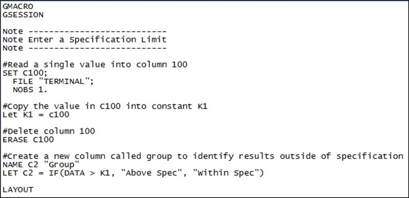
2. Add the following lines after the macro name and before the Layout command:

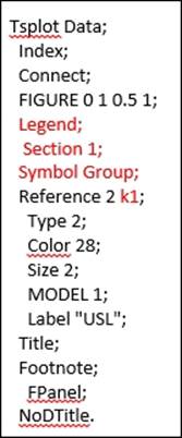
3. Find the Tsplot command in the macro. Change the Reference 2 12.5; line to Reference 2 K1;.

4. Add a Legend subcommand and a grouping symbol to the time series plot as shown in the following screenshot:

5. Save the macro and return to Minitab.

6. Press Ctrl + L to bring up the command-line editor and type %GSession and click on Submit Commands to run the macro.

How it works…

The Set command can be used to open data within ASCII files. Using the filename as a terminal, it specifies the session window as the data source. We could use a FORMAT subcommand with Set. The Format subcommand is used to set the format of the data; Fspecifies numeric values, A specifies the alphanumeric values, and DT specifies the date/time; more information on the format items can be found in Minitab's help section.

F5 tells Minitab to look for a five-digit number. Characters are included in that amount; for example, 12.5 is four characters. We could use the F3.1 format and it would read in three values, the last value being the first decimal place. For example, entering 123 with theF3.1 format would give us 12.3.

When the Format subcommand is not used, the Set command will only read in numeric values.

The last NObs subcommand is the number of observations. By fixing this to 1, we only look for one data entry. When the Set command is run, the session window will be given more focus and the prompt session will change to Data >; entering a value and pressingEnter will continue the macro.

The Set command can only read into columns, not constants. Because of this, we had to read into a column in the worksheet. It can be a safe practice to save the new data into columns that are away from the rest of the data to avoid any overwrites in new worksheets while storing data. The Let command then takes the value from C100 and enters this into the K1 constant. If there was more than one value in C100, we would specify the row with this syntax: C100[1].

We have used the # symbol to enter comments into the macro. Any text following a # is ignored by the macro. This can be in the line of the code as well.

We manually entered new subcommands to the time series plot command to group the symbols by the new group column. Alternatively, we could have made the changes on the graph and copied the command language. This is detailed in the previous recipe.

The Let command uses an IF statement as a calculator function. See the Calculator – using an if statement recipe in Chapter 1, Worksheet, Data Management, and the Calculator, to on how to calculate if statements. This is not the same as the IF session command that will be used in the Local macros with subcommands, submacros, and control statements recipe.

The Note command is a quick way to output notes into the session window. Any text that follows a note is printed to the session window. The Print command has a similar functionality but can also print columns or constants. The Print "Hello world" command will output text to the session window within the double quotes. The Print K1 command will print the value in the K1 constant.

There's more…

The reference line has been updated in this activity to take user input from the session window. Alternatively, we could place a reference line from the mean of the data. To do this, we would need to store the mean in a constant and use this constant for the reference line. The Column Statistics… tools under the Calc menu can be used to store values directly into constants.

Most of the Stat menu tools also offer us the ability to store values in the worksheet. These will be stored in the columns of the worksheet. This way, we can use many of the generated values and report them out on a new graphical page.

We may want the value that is generated by a function from a capability analysis such as Cpk, but may not want to generate the typical set of charts. In those cases, we can use the BRIEF command.

The BRIEF command can be used to limit or expand the output from results in Minitab. BRIEF 0 is no output; BRIEF 2 is the default level of output. The level of BRIEF relates to the options available in the results of many tools.

Some tools also have the NOCHART subcommand to suppress the graphical output.

See also

· The Calculator – using an if statement recipe in Chapter 1, Worksheet, Data Management, and the Calculator

· The Local macros with subcommands, submacros, and control statements recipe

Creating a Local macro

Local macros help create more general functions than Global macros or Execs. Rather than running from column references in the worksheet, we send data to a Local macro. This is run internally. On running a Local macro, we identify the data to be sent into the macro. We also need to declare the data type of variables used within the macro.

Here, we will convert the GSession macro from the previous recipe into a Local macro. This will allow us to tell the macro to use a column instead of looking for a specific column name or reference.

At this step, we will also simplify the function by removing the commands for the one sample t-test and one variance test.

Getting ready

Open the Macro data.MTW worksheet by using an open worksheet in the file menu. Then open the Gsession.mac file, which was created in Notepad in the previous recipe. Or, open the provided catch-up file.

How to do it…

The following commands will convert the Global macro from the previous recipe into a Local macro.

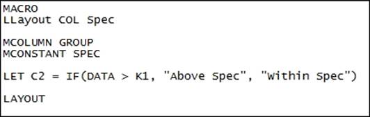
1. Go to the GSession.mac file. To prepare the file for our changes, save it as LLayout.mac in the macro directory.

2. In Notepad, remove the G from the start of GMACRO.

3. On the second line, change the name of the macro to LLAYOUT Col Spec.

4. Delete the commands associated with reading the data from the session window and replace these with the MColumn Col Group and MConstant Spec declarations. The initial lines of the macro till Layout should look as follows:

5. Replace all references of Data or 'Data' with Col.

6. Replace all references of K1 with Spec.

7. Replace any references of C2 with Group.

8. Delete the commands for the Onet One Sample t-test, and the OneVariance One Variance test.

9. Check if the macro looks similar to the following screenshot:

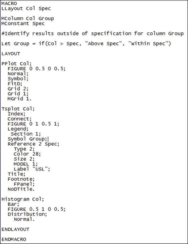
10. Save the macro and then go back to Minitab.

11. Press Ctrl + L to call up the command-line editor.

12. Enter %LLayout c1 12.5 into the command-line editor and click on Submit Commands to run the macro.

How it works…

The variables on the name line of the macro define how many items we need to specify when we run the macro; or rather, what information is passed to the macro. The Col command is the first value to be passed to the macro and Spec, the second.

Any variable used in the macro has to be declared. The MColumn command declares columns; MConstant is used for Spec to declare a constant. There are also MFree and MMatrix. The MFree command will allow the variable to be defined when the macro is invoked and is dependent on the variable type passed to the macro.

Variables can have any name as long as they do not clash with any of the commands in Minitab.

There's more…

Here, we have a macro that creates a panel of charts for any column that we send to the macro:

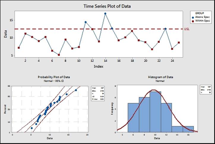
We can improve on this macro by allowing any number of columns to be used and making specifications optional.

The one sample t-test and one variance test were removed from the macro to simplify the example. If we wanted to keep the two tests, we could pass variables for the hypothesized mean and variance into the macro. When calling the macro, we would specify the data column, the specification, the mean, and the variance.

Another option to handle a lot of extra variables is to use subcommands on the macro name. Means and variances could be supplied as an optional command. If they are not used, the tests are not run; if they are supplied, then we would run the two tests. See the next recipe for an example of subcommands on the macro name.

See also

· The Local macros with subcommands, submacros, and control statements recipe

Local macros with subcommands, submacros, and control statements

This recipe will create a complicated macro using control statements and subcommands on the main macro command.

The following macro will be able to accept any number of columns on the main command line and generate a layout for each column. Specifications can be optional; they can be entered as a column or a single value. We will use a column for the specifications to allow different specifications for each column of data, or a constant to use the same specification for each column. The macro will be able to choose between the layout with or without specifications and perform an error check to see if the right number of specifications have been entered. This will cover several nested IF statements and DO loops.

Finally, we will copy the Llayout macro from the previous recipe into Notepad twice and edit this macro to create two submacros. One will be used to generate a layout for specifications and we will edit the other to create a layout when no specifications are used.

Getting ready

We will need the Llayout.mac file from the Creating a Local macro recipe or the catch-up file, Llayout.mac.

How to do it…

The following steps will convert the Llayout macro to use any number of columns as an input. We will also add a subcommand to use specifications as either a constant or a column:

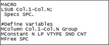
1. Open a new Notepad and save the file as LSub.mac in the macro folder.

2. Enter the values shown in the following screenshot into Notepad for the macro name, subcommand, and variables to be defined.

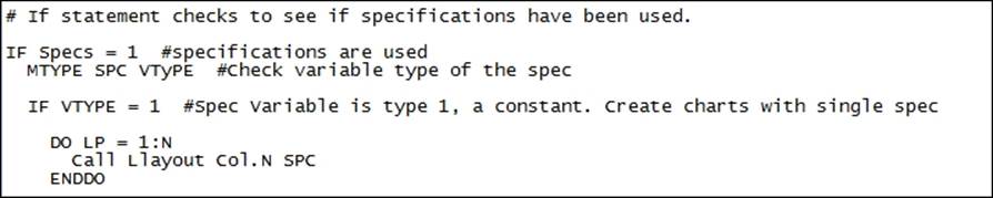
3. Enter the first part of the IF statements as a way to check if the specification subcommand has been used and to identify if it is a constant.

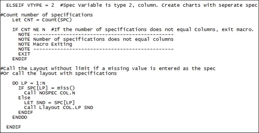
4. Enter the next section for the specifications that have been used as a column and to check if the number of specifications and the number of columns are the same.

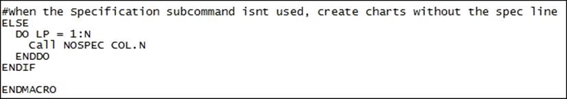
5. Finish the macro by entering the next section for no specifications used and ending the macro.

6. Copy the entire Llayout macro and paste this after ENDMACRO.

7. Paste the Llayout macro a second time.

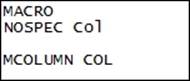
8. For the second Llayout commands, change the macro name to NOSPEC.

9. Delete all references to SPEC and GROUP from the NOSPEC macro.

10. Change the header section and declarations to the commands shown in the following screenshot:

11. Change the TSPLOT commands by removing the GROUP and Reference subcommands. Ensure that the TSPLOT command appears as follows:

12. Save the macro.

13. Return to Minitab and test the macro by first generating random data. Go to the Calc menu, then Random Data, and then select Normal….

14. In Number of rows of data to generate:, enter 30.

15. In the Store in column(s): section, enter c1-c5.

16. For the Mean: section, enter 10.

17. Click on OK.

18. In the worksheet, create a new column called Specifications.

19. Enter 11 11.5 * 12.5 13 in the Specifications column.

20. Press Ctrl + L to open the command-line editor.

21. Enter the %LSub c1-c5; command and press Enter to go to the next line.

22. Enter Specs c6. and click on Submit Commands.

How it works…

Subcommands that are entered on the macro name line allow optional commands to be entered. When running the macro, we can decide whether we want to use specifications or not.

The use of the Mfree command here allows a single specification to be entered as a constant; if separate specifications are desired, we can enter a column from the worksheet because Mfree will set its variable type based on the variable that is being passed to the macro. The Mtype command is then used to ask what variable type we have in SPC.

The first IF statement checks if the SPECS subcommand was used. If it was, then we check if the specifications were entered as a constant or column. If they are entered as a column, then we check if the number of specifications match the number of columns with the count of SPC compared to N.

To avoid rewriting the graph code several times, we store this in two separate macros: Llayout and Nospecs. If we want to remove excess code, we could further tidy this by placing the Pplot and the Histogram command in a third macro. As these commands haven't used specifications, using a third submacro could reduce the number of lines used.

The Miss() function is used to identify the missing values in the worksheet. It has been used here to identify when missing values have been entered for specifications. This allows us to not include a specification for some columns.

There's more…

The Default command can be used to fix the values of constants in subcommands. This allows us to set a value for these constants if they have not been specified when calling the macro. The Default command, though, must come directly after the declaration statements.