Neo4j High Performance (2015)
Chapter 2. Querying and Indexing in Neo4j
From what we learned in the previous chapter, we can say that while a relational database can be used to obtain the average age of all the people in a room, a graph database can indicate who is most likely to buy a drink. So, the utility of graph databases in the information age is vital.
In this chapter, we are going to take a look at the querying and indexing features of Neo4j and focus on the following areas:
· The Neo4j web interface
· Cypher queries and their optimization
· Introduction to Gremlin
· Indexing in Neo4j
· Migration techniques for SQL users
The Neo4j interface
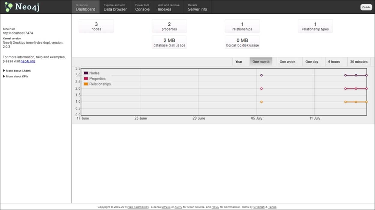
Neo4j comes with a browser-based web interface with the ability to manage your database, run queries in Cypher or REST, as well as visualization support for graphs. You can view the status of your database with a node and the relationship count and disk usage stats under dashboard. The data browser helps you to run queries and visualize the results in the form of a graph. You can use the console option to run queries on the database. Cypher and REST are supported in the console of the web interface. Gremlin support was deprecated in the recent version but you can always use it as a powerful external tool. Overall, the web interface provides developers with an easy-to-use system with a frontend for monitoring and querying.
Running Cypher queries
The default page when you open Neo4j is http://localhost:7474/browser/, and it is an interactive shell in the browser to execute your queries in a single or multiline format. You can also view the results locally in the timeline format along with tables or visualizations depending upon the query. Queries can be saved using the star button in the pane and the current content in the editor will be saved. Drag and drop of scripts for stored queries or data import is also possible in this interface.

For administrative purposes, you can redirect to the webadmin interface at http://localhost:7474/webadmin/, which houses several features and functions that can be used to manage and monitor your database system.
The Neo4j webadmin interface
Visualization of results
The most fascinating way of interacting with graphs is visualization. When you run Cypher queries, the result set is generally made up of nodes and relationships that are viewed in the data browser. Clicking on a node or a relationship in the visualizations will show a popup that contains the properties of that entity.
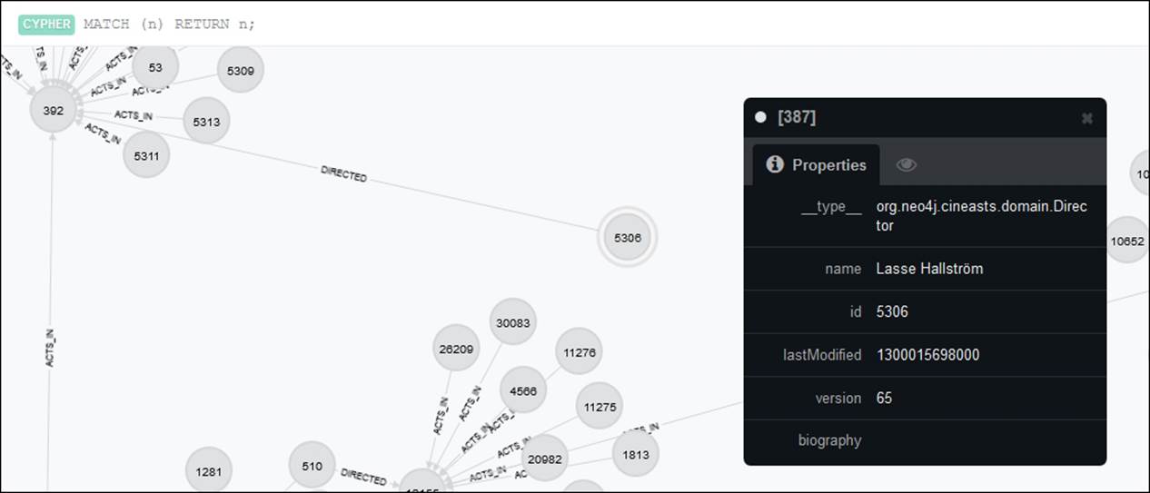
Visualization of results
You can also customize the content and colors, based on the label or type of relationship. A label is a named graph construct that is used to group nodes or relationships into sets; all nodes labeled with the same label belong to the same set. A type refers to different types of relationships that are present in the graph. (This is different from __type__, which is a property in Spring Data Neo4j used to map objects to nodes/relationships.) The elegance and design of Neo4j comes from the fact that every interaction that we have with it is a demonstration. It not only has a fluid and interactive UI but also a high-end administrative functionality.
Introduction to Cypher
Cypher is a graph query language that is declarative in nature. It supports expressive, efficient execution of queries and the updating of data on graph data stores. Cypher has a simple query construct but its power lies in the fact that we can express very complicated queries in a simple visual manner. This helps a developer to focus on the problem domain rather than worry about access issues of the database.
Cypher as a query language is humane by design. It is developer friendly as well as easily usable by an operations professional. Cypher's goal is making simple things easy and complex things possible; it bases its constructs on basic English prose, which makes queries increasingly self-explanatory. Since it is declarative in nature, Cypher emphasizes on expressing clearly what data has to be fetched from a graph, rather than how it is to be fetched, unlike most scripting and imperative languages such as Gremlin, or general-purpose programming languages such as Ruby or Java. In this approach, the optimization of queries becomes an implementation issue instead of going for the on-the-fly "updation" of traversals when the underlying structure or indexing of a database changes.
The Cypher syntax has been inspired by some well-established approaches for efficient querying. Some keywords in Cypher such as ORDER BY and WHERE are similar in functionality to those used in SQL. SPARQL-like (a primitive graph query language by Google) approaches for the matching of patterns have been adopted in Cypher; languages such as Python and Haskell have also inspired certain semantics.
Cypher graph operations
Cypher is a whiteboard-friendly language. Like the data on which it is used, queries in Cypher follow a diagrammatic approach in their syntax. This helps to target the use of graph databases to a greater variety of audience including database admins, developers, corporate professionals, and even the common folk. Let's take a look at some Cypher queries before diving into the best practices and optimizations for Cypher.
The following pattern shown depicts three entities interrelated through a relationship denoting the NEEDS dependency. It is represented in the form of an ASCII art:
(A)-[:NEEDS]->(B)-[:NEEDS]->(C), (A)-[:NEEDS]->(C)
The previous statement is in the form of a path that links entity A to B, then B to C, and finally A to C. The directed relation is denoted with the -> operator. As it is evident, patterns denoted in Cypher are a realization of how graphs are represented on a whiteboard. It is worth noting that although a graph can be constructed with edges in both directions, the query-processing languages operate in one direction, for example, from left to right as in the preceding case. This is handled using a list of patterns that are separated with commas. Cypher queries fundamentally make use of patterns of the ASCII art. What a cypher query does is hold on to some initiating part of the graph with a section of its pattern and then use the remaining parts of the pattern to search for local matching entities in the graph.
Cypher clauses
Being a language for querying data, Cypher consists of several clauses to perform different tasks. A simple basic operation with cypher makes use of the START clause to anchor to the source, which is succeeded by a MATCH clause that is used to conditionally traverse through desired nodes in the graph and finally a RETURN clause that outputs the matching values or some computable action result. In the following query, we find a connecting flight path for the city of Alabama using Cypher:
START city1=node:location(name='Alabama')
MATCH (city1)-[:CONNECTS]->(city2)-[:CONNECTS]->(city3), (city1)-[:CONNECTS]->(city3)
RETURN city2, city3
The preceding snippet contains the following three clauses:
· The START clause: This clause is used to indicate single or multiple starting points for the graph in consideration. The starting points in consideration can be nodes or relationships. We can look the start nodes up with the help of an index or occasionally accessed through the IDs of some node or relationship. In the previous query, we obtain the initial node with the help of an index called location that is asked to locate a place stored with the name property set to 'Alabama'. This statement returns a reference that we bind to an identifier called city1 in the previous example.
· The MATCH clause: These statements indicate that Cypher matches the pattern given with the initial identifier through the rest of the graph for find a match for the pattern. This way, we retrieve the data that we desire. Nodes are drawn with a set of parentheses and the relationships are indicated with the help of the --> and <-- symbols that also include the direction in which the relationship exists. Within the dashes in the previous symbols for relationships, we can insert the names of the relationships within a set of [ … ] and the name of the connecting relationship can be indicated after a colon.
Since the pattern in the MATCH clause can occur in many ways, and if the size of the dataset is increased manifold, we will get a very large set of matched results. To avoid this, we use anchoring for a part of the pattern with the help of the START clause.
The Cypher engine can then match the rest of the querying pattern in the graph surrounding the initiating points or nodes.
· The RETURN clause: The RETURN clause is used to specify the resulting nodes and connecting relationships that matched the pattern along with their properties in the form of identifiers, which in the previous example matched instances of city2 and city3. This follows a lazy binding approach for all the nodes that matched to some identifier that is specified in the query as the traversals take place in the graph.
More useful clauses
Some other essential clauses that Cypher supports for the construction of complex queries in the graph are listed as follows:
· CREATE: You can use this clause to define a new node or a new relationship. If you want only unique occurrences of nodes/relationships in the graphs, then you can use the CREATE UNIQUE clause to avoid the creation of duplicate entities.
· MERGE: This clause is equivalent to MATCH or CREATE. It can also be used with the help of indexes and unique constraints to find an existing entity or otherwise create a new one.
· WHERE: This clause provides a specification of conditions that can be used to filter nodes and relationships based on their stored properties.
· SET: This clause is used to assign values to properties of nodes or relationships.
· WITH: This clause is used to pipeline the output of one query in the form of input into the next query, thereby making the chaining of queries possible.
· UNION: This clause acts as a conjunction operation for queries in Cypher. You can combine the action of multiple queries on the data to produce a final result with the help of this clause.
· DELETE: It is used for the removal of any type of entities in the graph, be it nodes or relationships or their individual properties.
· FOREACH: This is an action clause that can be used to sequentially update the elements in a set of entities.
Some of these query clauses are radically similar to those in SQL. Cypher is intended to be simple enough so that it can be easily and quickly grasped by developers. Its clauses indicate that the operations are applied on graphs instead of relational data stores. We'll deal with some more clause-based examples in due course in the chapter.
Advanced Cypher tricks
Cypher is a highly efficient language that not only makes querying simpler but also strives to optimize the result-generation process to the maximum. A lot more optimization in performance can be achieved with the help of knowledge related to the data domain of the application being used to restructure queries.
Query optimizations
There are certain techniques you can adopt in order to get the maximum performance out of your Cypher queries. Some of them are:
· Avoid global data scans: The manual mode of optimizing the performance of queries depends on the developer's effort to reduce the traversal domain and to make sure that only the essential data is obtained in results. A global scan searches the entire graph, which is fine for smaller graphs but not for large datasets. For example:
· START n =node(*)
· MATCH (n)-[:KNOWS]-(m)
· WHERE n.identity = "Batman"
RETURN m
Since Cypher is a greedy pattern-matching language, it avoids discrimination unless explicitly told to. Filtering data with a start point should be undertaken at the initial stages of execution to speed up the result-generation process.
Note
In Neo4j versions greater than 2.0, the START statement in the preceding query is not required, and unless otherwise specified, the entire graph is searched.
The use of labels in the graphs and in queries can help to optimize the search process for the pattern. For example:
START n =node(*)
MATCH (n:superheroes)-[:KNOWS]-(m)
WHERE n.identity = "Batman"
RETURN m
Using the superheroes label in the preceding query helps to shrink the domain, thereby making the operation faster. This is referred to as a label-based scan.
· Indexing and constraints for faster search: Searches in the graph space can be optimized and made faster if the data is indexed, or we apply some sort of constraint on it. In this way, the traversal avoids redundant matches and goes straight to the desired index location. To apply an index on a label, you can use the following:
CREATE INDEX ON: superheroes(identity)
Otherwise, to create a constraint on the particular property such as making the value of the property unique so that it can be directly referenced, we can use the following:
CREATE CONSTRAINT ON n:superheroes
ASSERT n.identity IS UNIQUE
We will learn more about indexing, its types, and its utilities in making Neo4j more efficient for large dataset-based operations in the next sections.
· Avoid Cartesian Products Generation: When creating queries, we should include entities that are connected in some way. The use of unspecific or nonrelated entities can end up generating a lot of unused or unintended results. For example:
MATCH (m:Game), (p:Player)
This will end up mapping all possible games with all possible players and that can lead to undesired results. Let's use an example to see how to avoid Cartesian products in queries:
MATCH ( a:Actor), (m:Movie), (s:Series)
RETURN COUNT(DISTINCT a), COUNT(DISTINCT m), COUNT(DISTINCTs)
This statement will find all possible triplets of the Actor, Movie, and Series labels and then filter the results. An optimized form of querying will include successive counting to get a final result as follows:
MATCH (a:Actor)
WITH COUNT(a) as actors
MATCH (m:Movie)
WITH COUNT(m) as movies, actors
MATCH (s:Series)
RETURN COUNT(s) as series, movies, actors
This increases the 10x improvement in the execution time of this query on the same dataset.
· Use more patterns in MATCH rather than WHERE: It is advisable to keep most of the patterns used in the MATCH clause. The WHERE clause is not exactly meant for pattern matching; rather it is used to filter the results when used with START and WITH. However, when used with MATCH, it implements constraints to the patterns described. Thus, the pattern matching is faster when you use the pattern with the MATCH section. After finding starting points—either by using scans, indexes, or already-bound points—the execution engine will use pattern matching to find matching subgraphs. As Cypher is declarative, it can change the order of these operations. Predicates in WHERE clauses can be evaluated before, during, or after pattern matching.
· Split MATCH patterns further: Rather than having multiple match patterns in the same MATCH statement in a comma-separated fashion, you can split the patterns in several distinct MATCH statements. This process considerably decreases the query time since it can now search on smaller or reduced datasets at each successive match stage.
When splitting the MATCH statements, you must keep in mind that the best practices include keeping the pattern with labels of the smallest cardinality at the head of the statement. You must also try to keep those patterns generating smaller intermediate result sets at the beginning of the match statements block.
· Profiling of queries: You can monitor your queries' processing details in the profile of the response that you can achieve with the PROFILE keyword, or setting profile parameter to True while making the request. Some useful information can be in the form of_db_hits that show you how many times an entity (node, relationship, or property) has been encountered.
Returning data in a Cypher response has substantial overhead. So, you should strive to restrict returning complete nodes or relationships wherever possible and instead, simply return the desired properties or values computed from the properties.
· Parameters in queries: The execution engine of Cypher tries to optimize and transform queries into relevant execution plans. In order to optimize the amount of resources dedicated to this task, the use of parameters as compared to literals is preferred. With this technique, Cypher can re-utilize the existing queries rather than parsing or compiling the literal-hbased queries to build fresh execution plans:
· MATCH (p:Player) –[:PLAYED]-(game)
· WHERE p.id = {pid}
RETURN game
When Cypher is building execution plans, it looks at the schema to see whether it can find useful indexes. These index decisions are only valid until the schema changes, so adding or removing indexes leads to the execution plan cache being flushed.
Add the direction arrowhead in cases where the graph is to be queries in a directed manner. This will reduce a lot of redundant operations.
Graph model optimizations
Sometimes, the query optimizations can be a great way to improve the performance of the application using Neo4j, but you can incorporate some fundamental practices while you define your database so that it can make things easier and faster for usage:
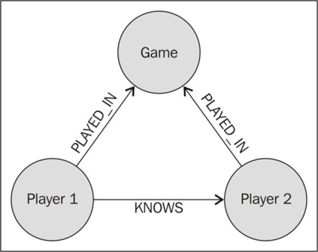
· Explicit definition: If the graph model we are working upon contains implicit relationships between components. A higher efficiency in queries can be achieved when we define these relations in an explicit manner. This leads to faster comparisons but it comes with a drawback that now the graph would require more storage space for an additional entity for all occurrences of data. Let's see this in action with the help of an example.
In the following diagram, we see that when two players have played in the same game, they are most likely to know each other. So, instead of going through the game entity for every pair of connected players, we can define the KNOWS relationship explicitly between the players.
· Property refactoring: This refers to the situation where complex time-consuming operations in the WHERE or MATCH clause can be included directly as properties in the nodes of the graph. This not only saves computation time resulting in much faster queries but it also leads to more organized data storage practices in the graph database for utility. For example:
· MATCH (m:Movie)
· WHERE m.releaseDate >1343779201 AND m.releaseDate< 1369094401
RETURN m
This query is to compare whether a movie has been released in a particular year; it can be optimized if the release year of the movie is inherently stored in the properties of the movie nodes in the graph as the year range 2012-2013. So, for the new format of the data, the query will now change to this:
MATCH (m:Movie)-[:CONTAINS]->(d)
WHERE s.name = "2012-2013"
RETURN g
This gives a marked improvement in the performance of the query in terms of its execution time.
Gremlin – an overview
Gremlin is basically a wrapper to Groovy. It provides some nice constructs that make the traversal of graphs efficient. It is an expressive language written by Marko Rodriguez and uses connected operations for the traversal of a graph. Gremlin can be consideredTuring complete and has simple and easy-to-understand syntax.
Note
Groovy is a powerful, optionally typed, and dynamic language, with static typing and static compilation capabilities for the Java platform aimed at multiplying developers' productivity thanks to a concise, familiar, and easy-to-learn syntax. It integrates smoothly with any Java program and immediately delivers to your application powerful features, including scripting capabilities, domain-specific language authoring, runtime and compile-time meta-programming, and functional programming. Check it out at http://groovy-lang.org/.
Gremlin integrates well with Neo4j since it was mainly designed for use with property graphs. The earlier versions sported the Gremlin console on the web interface shell, but the latest version does away with it. Gremlin is generally used with an REPL or a command line to make traversals on a graph interactively.
Let's browse through some useful queries in Gremlin for graph traversals.
You can set up the Gremlin REPL to test out the queries. Download the latest build from https://github.com/tinkerpop/gremlin/wiki/Downloads and follow the setup instructions given on the official website. Now, in order to configure your Gremlin with your Neo4j installation, you need to first create a neo4j.groovy file with the path to your neo4j/data/graph.db directory and add the following lines:
// neo4j.groovy
import org.neo4j.kernel.EmbeddedReadOnlyGraphDatabase
db = new EmbeddedReadOnlyGraphDatabase('/path/to/neo4j/data/graph.db')
g = new Neo4jGraph(db)
When you start a new Gremlin REPL, you will need to load this file in order to use Gremlin commands with your Neo4j database:
$ cd /path/to/gremlin
$ ./gremlin.sh
\,,,/
(o o)
-----oOOo-(_)-oOOo-----
gremlin> load neo4j.groovy
gremlin>
You can now try out some of the Gremlin clauses mentioned in the following points:
· You can connect to an existing instance of a graph database such as Neo4j with the help of the following command at the Gremlin prompt:
· gremlin> g = new Neo4jGraph ("/path/to/database")
· If you want to view all the nodes or vertices and edges in the graph, you can use the following commands:
· gremlin> g.V
· gremlin> g.E
· To get a particular vertex that has been indexed, type the following command. It returns the vertex that has a property name "Bill Gates" as the name. Since the command returns an iterator, the >> symbol is used to pop the next item in the iterator and assign it to the variable in consideration:
· gremlin> v = g.idx(T.v)[[name: "Bill Gates"]] >> 1
· ==>v[165]
· To look at the properties on the particular vertex, you need the following command:
· gremlin> v.map
· ==> name = Bill Gates
· ==> age = 60
· ==> designation = CEO
· ==> company = Microsoft
To view the outgoing edges from that node, we use the following command. The result of that will print out all the outbound edges from that graph in the format that consists of the node indices:
e[212][165-knows->180]
==> v.outE
· You can also write very simple queries to retrieve the node at the other end of a relationship based on its label in the following manner:
· gremlin> v.outE[[label:'knows']].inV.name
· ==> Steve Jobs
· Gremlin also allows you to trace the path it takes to achieve a particular result with the help of an in-built property. All you need to do is append a .path to the end of the query whose path you want to view:
· gremlin> v.outE[[label:'knows']].inV.name.path
· ==> [v[165], e[212][ 165-knows->180], v[180], Steve Jobs]
· If we need to find the names of all the vertices in the graph that are known by the vertex with the ID 165 and that have exceeded 30 years. Note that conditions in the Gremlin statements are expressed in a pair of {} similar to that in Groovy:
· gremlin> v.outE{it.label=='knows'}.inV{it.age > 30}.name
· Finally, let's see how we can use collaborative filters on the vertex with the ID 165 to make calculations:
· gremlin> m = [:]
· gremlin> v.outE.inV.name.groupCount(m).back(2).loop(3){it.loops<4}
· gremlin> m.sort{a,b -> a.value <=> b.value}
The preceding statements first create a map in Groovy called m. Next, we find all the outgoing edges from v, the incoming vertices at the end of those edges, and then the name property. Since we cannot get the outgoing edges of the name, we go back two steps to the actual vertex and then loop back three times in the statement to go to the required entity. This maps the count retrieved from the looping to the ID of the vertex and then stores them in the m map. The final statement sorts the results in the map based on the count value. So, Gremlin is quite interesting for quick tinkering with graph data and constructing small complex queries for analysis. However, since it is a Groovy wrapper for the Pipes framework, it lacks scope for optimizations or abstractions.
Indexing in Neo4j
In earlier builds, Neo4j had no support for indexing and was a simple property graph. However, as the datasets scaled in size, it was inconvenient and error-prone to traverse the entire graph for even the smallest of queries, so the need to effectively define the starting point of the graph had to be found. Hence, the need for indexing arose followed by the introduction of manual and then automatic indexing. Current versions of Neo4j have extensive support for indexing as part of their fundamental graph schema.
Manual and automatic indexing
Manual indexing was introduced in the early versions of Neo4j and was achieved with the help of the Java API. Automatic indexing was introduced from Neo4j 1.4. It's a manual index under the hood that contains a fixed name (node_auto_index, relationship_auto_index) combined with TransactionEventHandler that mirrors changes on index property name configurations. Automatic indexing is typically set up in neo4j.properties. This technique removes lot of burden from the manual mirroring of changes to the index properties, and it permits Cypher statements to alter the index implicitly. Every index is bound to a unique name specified by the user and can be associated with either a node or a relationship. The default indexing service in Neo4j is provided by Lucene, which is an Apache project that is designed for high-performance text-search-based projects. The component in Neo4j that provides this service is known as neo4j-lucene-index and comes packaged with the default distribution of Neo4j. You can browse its features and properties at http://repo1.maven.org/maven2/org/neo4j/neo4j-lucene-index/. We will look at some basic indexing operations through the Java API of Neo4j.
Creating an index makes use of the IndexManager class using the GraphDatabaseService object. For a graph with games and players as nodes and playing or waiting as the relationships, the following operations occur:
//Create the index reference
IndexManager idx = graphDb.index();
//Index the nodes
Index<Node> players = idx.forNodes( "players" );
Index<Node> games = idx.forNodes( "games" );
//Index the relationships in the graph
RelationshipIndex played = idx.forRelationships( "played" );
For an existing graph, you can verify that an entity has been indexed:
IndexManager idx = graphDb.index();
boolean hasIndexing = idx.existsForNodes( "players" );
To add an entity to an index service, we use the add(entity_name) method, and then for complete removal of the entity from the index, we use the remove ("entity name") method. In general, indexes cannot be modified on the fly. When you need to change an index, you will need to get rid of the current index and create a new one:
IndexHits<Node> result = players.get( "name", "Ronaldo" );
Node data = result.getSingle();
The preceding lines are used to retrieve the nodes associated with a particular index. In this case, we get an iterator for all nodes indexed as players who have the name Ronaldo. Indexes in Neo4j are useful to optimize the queries. Several visual wrappers have been developed to view the index parameters and monitor their performance. One such tool is Luke, which you can view at https://code.google.com/p/luke/.
Having told Neo4j we want to auto-index relationships and nodes, you might expect it to be able to start searching nodes straightaway, but in fact, this is not the case. Simply switching on auto-indexing doesn't cause anything to actually happen. Some people find that counterintuitive and expect Neo4j to start indexing all node and relationship properties straight away. In larger datasets, indexing everything might not be practical since you are potentially increasing storage requirements by a factor of two or more with every value stored in the Neo4j storage as well as the index. Clearly, there will also be a performance overhead on every mutating operation from the extra work of maintaining the index. Hence, Neo4j takes a more selective approach to indexing, even with auto-indexing turned on; Neo4j will only maintain an index of node or relationship properties it is told to index. The strategy here is simple and relies on the key of the property. Using the config map programmatically requires the addition of two properties that contain a list of key names to index as shown below.
Schema-based indexing
Since Neo4j 2.0, there is extended support for indexing on graph data, based on the labels that are assigned to them. Labels are a way of grouping together one or more entities (both nodes and relationships) under a single name. Schema indexed refers to the process of automatically indexing the labeled entities based on some property or a combination of properties of those entities. Cypher integrates well with these new features to locate the starting point of a query easily.
To create a schema-based index on the name_of_player property for all nodes with the label, you can use the following Cypher query:
CREATE INDEX ON :Player(name_of_player)
When you run such a query on a large graph, you can compare the trace of the path that Neo4j follows to reach the starting node of the query with and without indexing enabled. This can be done by sending the query to the Neo4j endpoint in your database machine in a curl request with the profile flag set to true so that the trace is displayed.
curl http://localhost:7474/db/data/cypher?profile=true -H "Accept: application/json" -X POST -H "Content-type: application/json" --data '{"query" : "match pl:Player where pl.name_of_player! = \"Ronaldo\" return pl.name_of_player, pl.country"}'
The result that is returned from this will be in the form of a JSON object with a record of how the execution of the query took place along with the _db_hits parameter that tells us how many entities in the graph were encountered in the process.
The performance of the queries will be optimized only if the most-used properties in your queries are all indexed. Otherwise, Neo4j will have no utility for the indexing if it has one property indexed and the retrieval of another property match requires traversing all nodes. You can aggregate the properties to be used in searches into a single property and index it separately for improved performance. Also, when multiple properties are indexed and you want the index only on a particular property to be used, you can specify this using the following construct using the p:Player(name_of_player) index with schema indexes; we no longer have to specify the use of the index explicitly. If an index exists, it will be used to process the query. Otherwise, it will scan the whole domain. Constraints can be used with similar intent as the schema indexes. For example, the following query asserts that the name_of_player property in the nodes labeled as Player is unique:
CREATE CONSTRAINT ON (pl:Player) ASSERT player.name_of_player IS UNIQUE
Currently, schema indexes do not support the indexing of multiple properties of the label under a same index. You can, however, use multiple indexes on different properties of nodes under the same label.
Indexing takes up space in the database, so when you feel an index is no longer needed, it is good to relieve the database of the burden of such indexes. You can remove the index from all labeled nodes using the DROP INDEX clause:
DROP INDEX ON :Player(name_of_player)
The use of schema indices is much simpler in comparison to manual or auto-indexing, and this gives an equally efficient performance boost to transactions and operations.
Indexing benefits and trade-offs
Indexing does not come for free. Since the underlying application code is responsible for the management and use of indexes, the strategy that is followed should be thought over carefully. Inappropriate decisions or flaws in indexing result in decreased performance or unnecessary use of disk storage space.
High on the list of trade-offs for indexing is the fact that an index result uses storage, that is, the higher the number of entities that are indexed, the greater the disk usage. Creating indexes for the data is basically the process of creating small lookup maps or tables to allow rapid access to the data in the graph. So, for write operations such as INSERT or UPDATE, we write the data twice, once for the creation of the node and then to write it to the index mapping, which stores a pointer to the created node.
Moreover, with an elevated number of indexes, operations for insertions and updates will take a considerable amount of time since nearly as many operations are performed to index as compared to creating or updating entities. The code base will naturally scale since updates/inserts will now require the modification of the index for that entity and as is observed, if you profile the time of your query, the time to insert a node with indexes is roughly twice of that when inserted without indexes.
On the other hand, the benefit of indexing is that query performance is considerably improved since large sections of the graph are eliminated from the search domain.
Note that storing the Neo4j-generated IDs externally in order to enable fast lookup is not a good practice, since the IDs are subject to alterations. The ID of nodes and relationships is an internal representation method, and using them explicitly might lead to broken processes.
Therefore, the indexing scenario would be different for different applications. Those that require updation or creation more frequently than reading operations should be light in indexing entities, whereas applications dealing primarily with reads should generously use indexes to optimize performance.
Migration techniques for SQL users
Neo4j has been around for just a few years, while most organizations that are trying to move into business intelligence and analytics have their decades of data piled up in SQL databases. So, rather than moving or transforming the data, it is better to fit in a graph database along with the existing one in order to make the process a less disruptive one.
Handling dual data stores
The two databases in our system are arranged in a way that the already-in-place MySQL database will continue being the primary mode of storage. Neo4j acts as the secondary storage and works on small related subsets of data. This would be done in two specific ways:
· Online mode for transactions that are critical for essential business decisions that are needed in real time and are operated on current sets of data
· The system can also operate in batch mode in which we collect the required data and process it when feasible
This will require us to first tune our Neo4j system to get updated with the historical data already present in the primary database system and then adapt the system to sync between the two data stores.
We will try to avoid data export between the two data stores and design the system without making assumptions about the underlying data model.
Analyzing the model
Let's use a simple entity set of people buying cars sold by dealers to illustrate the process. You can fit in the process to your existing data setup. We outline the features of the objects in our domains as follows:
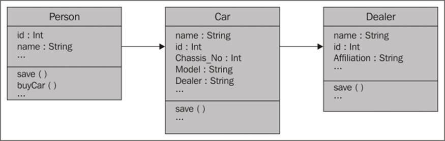
The SQL schema of an existing database
We can represent the corresponding model in Neo4j as a directed acyclic graph. The corresponding Neo4j acyclic graph handles the persistence with the database. Mutating Cypher is used to transform the data into a graph that contains nodes and relationships using the API of Neo4j in certain cases so that complex objects can be handled. Each entity relates back to the underlying database with the help of an ID that acts as the system's primary key and indexing operations are performed on this key. The corresponding graph model is as follows:
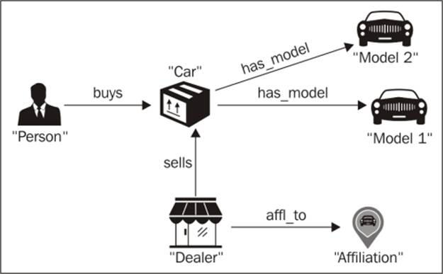
The corresponding representation in a graph database
When the graph modeling is complete, our application becomes independent of our primary data store.
Initial import
We now have to initiate the import of our data and store it after transformation into the form of our graph objects. We use SQL queries in order to obtain the required data by reading from the database, or requesting an existing API or previously exported set of data.
//Update a person node or create one. If created, its id is indexed.
SELECT name, id from person where
Person person=new Person(res.getString("name"), res.getInt("id"));
person.save();
//Update a car or create one. If created, its id is indexed.
SELECT name, id from car where
Car car=new Car(res.getString("name"),res.getInt("id"));
car.save();
//Update a dealer or create one. An "affiliation" node is created if not already existing. A relationship is created to the affiliation from the dealer. The ids of both dealer and affiliation are indexed.
SELECT name, id, affiliation from dealers where
Dealer dealer=new Dealer(res.getString("name"), res.getInt("id"));
dealer.setAffiliation(res.getString("affiliation"));
dealer.save();
//A relationship is created to the car from the person and we set the date of buying as a property of that relationship
SELECT person.id, car.id, buying_date from Purchase_Table
Person person=repository.getById(res.getInt("customer.id"));
person.buyCar(res.getInt("id"),res.getDate("buying_date");
Note that the preceding queries are abstract and will not run standalone. They illustrate the method of integrating with a relational database. You can change them according to your relational database schema.
Keeping data in sync
Having successfully imported data between the systems, we are now required to keep them in sync. For this purpose, we can schedule a cron job that will perform the previous operations in a periodic manner. You can also define an event-based trigger that will report on updates, such as cars being bought or new customers joining, in the primary system and incorporate them in the Neo4j application.
This can be implemented with simple concepts, such as message queues, where you can define the type of message required to be used by our secondary database system. Regardless of the content of the message, our system should be able to read and parse the message and use it for our business application logic.
The result
There is a loose coupling between the applications and we have used an efficient parsing approach to adapt the data between multiple formats. Although this technique works well for most situations, the import process might require a slightly longer time initially due to the transactional nature, but the initial import is not a process that occurs frequently. The sync based on events is a better approach in terms of performance.
You need an in-depth understanding of the data pattern in your application so that you can decide which technique is suitable. For single-time migrations of large datasets, there are several available tools such as the batch importer (https://github.com/jexp/batch-import) or the REST batch API on a database server that runs Neo4j.
Useful code snippets
Data storage and operations on data are essentially well framed and documented for Neo4j. When it comes to the analysis of data, it is much easier for the data scientists to get the data out of the database in a raw format, such as CSV and JSON, so that it can be viewed and analyzed in batches or as a whole.
Importing data to Neo4j
Cypher can be used to create graphs or include data in your existing graphs from common data formats such as CSV. Cypher uses the LOAD CSV command to parse CSV data into the form that can be incorporated in a Neo4j graph. In this section, we demonstrate this functionality with the help of an example.
We have three CSV files: one contains players, the second has a list of games, and the third has a list of which of these players played in each game. You can access the CSV files by keeping them on the Neo4j server and using file://, or by using FTP, HTTP, or HTTPS for remote access to the data.
Let's consider sample data about cricketers (players) and the matches (games) that were played by them. Your CSV file would look like this:
id,name
1,Adam Gilchrist
2,Sachin Tendulkar
3,Jonty Rhodes
4,Don Bradman
5,Brian Lara
You can now load the CSV data into Neo4j and create nodes out of them using the following commands, where the headers are treated as the labels of the nodes and the data from every line is treated as nodes:
LOAD CSV WITH HEADERS FROM "http://192.168.0.1/data/players.csv" AS LineOfCsv
CREATE (p:Person { id: toInt(LineOfCsv.id), name: LineOfCsv.name })
Now, let's load the games.csv file. The format of the game data will be in the following format where each line would have the ID, the name of the game, the country it was played in, and the year of the game:
id,game,nation,year
1,Ashes,Australia,1987
2,Asia Cup,India,1999
3,World Cup,London,2000
The query to import the data would now also have the code to create a country node and relate the game with that country:
LOAD CSV WITH HEADERS FROM " http://192.168.0.1/data/games.csv" AS LineOfCsv
MERGE (nation:Nation { name: LineOfCsv.nation })
CREATE (game:Game { id: toInt(LineOfCsv.id), game: LineOfCsv.game, year:toInt(LineOfCsv.year)})
CREATE (game)-[:PLAYED_IN]->(nation)
Now, we go for importing the relationship data between the players and the games to complete the graph. The association would be many to many in nature since a game is related to many players and a player has played in many games; hence, the relationship data is stored separately. The user-defined field id in players and games needs to be unique for faster access while relating and also to avoid conflicts due to common IDs in the two sets. Hence, we index the ID fields from both the previous imports:
CREATE CONSTRAINT ON (person:Person) ASSERT person.id IS UNIQUE
CREATE CONSTRAINT ON (movie:Movie) ASSERT movie.id IS UNIQUE
To import the relationships, we read a line from the CSV file, find the IDs in players and games, and create a relationship between them:
USING PERIODIC COMMIT
LOAD CSV WITH HEADERS FROM "http://path/to/your/csv/file.csv" AS csvLine
MATCH (player:Player { id: toInt(csvLine.playerId)}), (game:Game { id: toInt(csvLine.movieId)})
CREATE (player)-[:PLAYED {role: csvLine.role }]->(game)
The CSV file that is to be used for snippets such as the previous one will vary according to the dataset and operations at hand, a basic version of which is represented here:
playerId,gameId,role
1,1,Batsman
4,1,WicketKeeper
2,1,Batsman
4,2,Bowler
2,2,Bowler
5,3,All-Rounder
In the preceding query, the use of PERIODIC COMMIT indicates to the Neo4j system that the query can lead to the generation of inordinate amounts of transaction states and therefore would require to be committed periodically to the database instead of once at the end. Your graph is now ready. To improve efficiency, you can remove the indexing from the id fields and also the field themselves the nodes since they were only needed for the creation of the graph.
Exporting data from Neo4j
Inherently, Neo4j has no direct format to export data. For the purpose of relocation or backup, the Neo4j database as a .db file can be stored, which is located under the DATA directory of your Neo4j base installation directory.
Cypher query results are returned in the form of JSON documents, and we can directly export the json documents by using curl to query Neo4j with Cypher. A sample query format is as follows:
curl -o output.json -H accept:application/json -H content-type:application/json --data '{"query" : "your_query_here" }' http://127.0.0.1:7474/db/data/cypher
You can also use the structr graph application platform (http://structr.org) to export data in the CSV format. The following curl format is used to export all the nodes in the graph:
curl http://127.0.0.1:7474/structr/csv/node_interfaces/export
To export relationships using the structr interface, the following commands are used:
curl http://127.0.0.1:7474/structr/csv/node_interfaces/out
curl http://127.0.0.1:7474/structr/csv/node_interfaces/in
These store the incoming and outgoing relationships in the graph. Although the two sets of results overlap, this is necessary with respect to nodes in order to retrieve the graph. A lot more can be done with structr other than exporting data, which you can find at its official website. Apart from the previously mentioned techniques, you can always use the Java API for retrieval by reading the data by entity, transforming it into your required format (CSV/JSON), and writing it to a file.
Summary
In this chapter, you learned about Cypher queries, the clauses that give Cypher its inherent power, and how to optimize your queries and data model in order to make the query engine robust. We saw the best practices for improved performance using the types of indexing we can use on our data including manual, auto, and schema-based indexing practices.
In the next chapter, we will look at graph models and schema design patterns while working with Neo4j.
All materials on the site are licensed Creative Commons Attribution-Sharealike 3.0 Unported CC BY-SA 3.0 & GNU Free Documentation License (GFDL)
If you are the copyright holder of any material contained on our site and intend to remove it, please contact our site administrator for approval.
© 2016-2026 All site design rights belong to S.Y.A.