Joe Celko's Complete Guide to NoSQL: What Every SQL Professional Needs to Know about NonRelational Databases (2014)

Chapter 3. Graph Databases

Abstract

Graph databases model relationships, not data. Just as SQL and RDBMS are based on logic and set theory, graph databases are based on graph theory. The classic example of a popular graph problem is called the “Kevin Bacon problem” in the literature. Given actor Kevin Bacon, a graph database links him to anyone else in the movie industry either by a direct link (had some role in a movie with Kevin Bacon) or by a chain of links (had some role in a movie with someone who had some role in a movie with Kevin Bacon). However, other graph problems look for the shortest paths among a set of paths in a transportation network, the smallest set of nodes that cover a graph, and so forth. There is no ANSI/ISO standard language for graphs, but the most popular ones are Gremlin, Neo4j, and SPARQL. They tend to model their syntax after SQL and/or mathematics.

Keywords

graph theory; Gremlin; Kevin Bacon problem; Neo4j; SPARQL

Introduction

This chapter discusses graph databases, which are used to model relationships rather than traditional structured data. Graph databases have nothing to do with presentation graphics. Just as FORTRAN is based on algebra, and relational databases are based on sets, graph databases are based on graph theory, a branch of discrete mathematics. Here is another way we have turned a mind tool into a class of programming tools!

Graph databases are not network databases. Those were the prerelational databases that linked records with pointer chains that could be traversed record by record. IBM's Information Management System (IMS) is one such tool still in wide use; it is a hierarchical access model. Integrated Database Management System (IDMS), TOTAL, and other products use more complex pointer structures (e.g., single-link lists, double-linked lists, junctions, etc.) to allow more general graphs than just a tree. These pointer structures are “hardwired” so that they can be navigated; they are the structure in which the data sits.

In a graph database, we are not trying to do arithmetic or statistics. We want to see relationships in the data. Curt Monash the database expert and blogger (http://www.dbms2.com/, http://www.monash.com) coined the term for this kind of analysis: relationship analytics.

Programmers have had algebra in high school, and they may have had some exposure to naive set theory in high school or college. You can program FORTRAN and other procedural languages with high school–level algebra and only a math major needs advanced set theory, which deals with infinite sets (computers do not have infinite storage no matter what your boss thinks). But you cannot really understand RDBMS and SQL without naive set theory.

But only math majors seem to take a whole semester of graph theory. This is really too bad; naive graph theory has simple concepts and lots of everyday examples that anyone can understand. Oh, did I mention that it is also full of sudden surprises where simple things become nonpolynomial (NP)-complete problems? Let’s try to make up that gap in your education.

In computer science, we use the “big O” notation, O(n), to express how much effort it takes to run an algorithm as the size of the input, (n). For example, if we have a simple process that handles one record at a time, the O(n) is linear; add one more record and it takes one more unit of execution time. But some algorithms increase in more complex ways. For example, sorting a file can be done in O(n log₂(n)) time. Other algorithms can have a complexity that is a polynomial usually with squares and cubes. Then we get to the NP algorithms. They usually involve having to try all possible combinations to find a solution, so they have a factorial in their complexity, O(n!).

NP complexity shows up in many of the classic graph theory problems. Each new edge or node added to the graph can result in more and more combinations. We often find that we look for near-optimal solutions instead of practical reasons.

3.1 Graph Theory Basics

A graph has two things in it. There are edges (or arcs) and nodes (or vertices); the edges are drawn as lines that connect nodes, which are drawn as dots or circles. That is it! Two parts! Do not be fooled; binary numbers only have two parts and we build computers with them.

3.1.1 Nodes

Nodes are abstractions. They usually (not always) model what would be an entity in RDBMS. In fact, some of the power of graph theory is that a node can model a subgraph. A node may or may not have “something inside it” (electrical components) in the model; it can just sit there (bus stop) or simply be (transition state). A node is not an object. Objects have methods and local data inside them. In a complex graph query, we might be looking for an unknown or even nonexistent node. For example, a bus stop with a Bulgarian barbeque stand might not exist. But a bus stop with a barbeque in a Bulgarian neighborhood might exist, and we not do know it until we connect many factors together (e.g., riders getting off at the Bulgarian Culture Center bus stop, restaurants or Bulgarian churches within n blocks of the bus stop, etc.). Other examples of graphs you might have seen are:

◆ Schematic maps: the nodes are the bus stops, towns, and so forth.

◆ Circuit diagrams: the nodes are electrical components.

◆ State transitions: the nodes are the states (yes, this can be modeled in SQL).

3.1.2 Edges

Edges or arcs connect nodes. We draw them as lines that may or may not have an arrow head on them to show a direction of flow. In schematic maps, the edges are the roads. They can have a distance or time on them. In the circuit diagrams, the edges are the wires that have resistance, voltage, etc. Likewise, the abstract state transitions are connected by edges that model the legal transition paths.

In one way, edges are more fun than nodes in graph theory. In RDBMS models of data, we have an unspecified single relationship between tables in the form of a REFERENCES clause. In a graph database, we can have multiple edges of different kinds between nodes. These can be of various strengths that we know (e.g., “I am your father, Luke,” if you are a Star Wars fan; “is a pen pal of”) and ones that we establish from other sources (e.g., “subscribes to the Wall Street Journal”; “friend of a friend of a friend”; “son of a son of a sailor,” if you are a Jimmy Buffett fan).

At the highest level of abstraction an edge can be directed or undirected. In terms of maps, these are one-way streets; for state transitions, this is prior state–current state pairs and so forth. We tend to like undirected graphs since the math is easier and there is often an inverse relationship of some sort (e.g., “father–son” in the case of Luke Skywalker and Darth Vader).

Colored edges are literally colored lines on a display of a graph database. One color is used to show the same kind of edge, the classic “friend of a friend of a friend,.” or a Bacon(n) relationship (I will explain this shortly) used in social networks when they send you a “you might also know …” message and ask you to send an invitation to that person to make a direct connection.

Weighted edges have a measurement that can accumulate. In the case of a map—distances—the accumulation rule is additive; in the case of the Bacon(n) function it diminishes over distance (you may ask, “Who? Oh, I forgot about him!”).

3.1.3 Graph Structures

The bad news is that since graph theory is fairly new by mathematical standards, which means less than 500 years old, there are still lots of open problems and different authors will use different terminology. Let me introduce some basic terms that people generally agree on:

◆ A null graph is a set of nodes without any edges. A complete graph has an edge between every pair of nodes. Both of these extremes are pretty rare in graph databases.

◆ A walk is a sequence of edges that connect a set of nodes without repeating an edge.

◆ A connected graph is a set of nodes in which any two nodes can be reached by a walk.

◆ A path is a walk that goes through each node only once. If you have n nodes, you will have (n − 1) edges in the path.

◆ A cycle or circuit is a path that returns to where it started. In RDBMS, we do not like circular references because referential actions and data retrieval can hang in an endless loop. A Hamiltonian circuit is one that contains all nodes in a graph.

◆ A tree is a connected graph that has no cycles. I have a book on how to model trees and hierarchies in SQL (Celko, 2012). Thanks to hierarchical databases, we tend to think of a directed tree in which subordination starts at a root node and flows down to leaf nodes. But in graph databases, trees are not as obvious as an organizational chart, and finding them is a complicated problem. In particular, we can start at a node as the root and look for the minimal spanning tree. This is a subset of edges that give us the shortest path from the root we picked to each node in the graph.

Very often we are missing the edges we need to find an answer. For example, we might see that two people got traffic tickets in front of a particular restaurant, but this means nothing until we look at their credit card bills and see that these two people had a meal together.

3.2 RDBMS Versus Graph Database

As a generalization, graph databases worry about relationships, while RDBMSs worry about data. RDBMSs have difficulties with complex graph theoretical analysis. It’s easy to manage a graph where every path has length one; that is just a three-column table (node, edge, node). By doing self-joins, you can construct paths of length two, and so forth, called a breadth-first search. If you need a mental picture, think of an expanding search radius. You quickly get into Cartesian explosions for longer paths, and can get lost in an endless loop if there are cycles. Furthermore, it is extremely hard to write SQL for graph analysis if the path lengths are long, variable, or not known in advance.

3.3 Six Degrees of Kevin Bacon Problem

The game “Six Degrees of Kevin Bacon” was invented in 1994 by three Albright College students: Craig Fass, Brian Turtle, and Mike Ginelli. They were watching television movies when the film Footloose was followed by The Air Up There, which lead to the speculation that everyone in the movie industry was connected in some way to Kevin Bacon. Kevin Bacon himself was assigned the Bacon number 0; anyone who had been in a film with him has a Bacon number of 1; anyone who worked with that second person has a Bacon number of 2; and so forth. The goal is to look for the shortest path. As of mid-2011, the highest finite Bacon number reported by the Oracle of Bacon is 8.

This became a fad that finally resulted in the website “Oracle of Bacon” (http://oracleofbacon.org), which allows you to do online searches between any two actors in the Internet Movie Database (www.imdb.com). For example, Jack Nicholson was in A Few Good Menwith Kevin Bacon, and Michelle Pfeiffer was in Wolf with Jack Nicholson. I wrote a whitepaper for Cogito, Inc. of Draper, UT, in which I wrote SQL queries to the Kevin Bacon problem as a benchmark against their graph database. I want to talk about that in more detail.

3.3.1 Adjacency List Model for General Graphs

Following is a typical adjacency list model of a general graph with one kind of edge that is understood from context. Structure goes in one table and the nodes in a separate table, because they are separate kinds of things (i.e., entities and relationships). The SAG card number refers to the Screen Actors Guild membership identifier, but I am going to pretend that they are single letters in the following examples.

CREATE TABLE Actors

(sag_card CHAR(9) NOT NULL PRIMARY KEY

actor_name VARCHAR(30) NOT NULL);

CREATE TABLE MovieCasts

(begin_sag_card CHAR(9) NOT NULL

REFERENCES Nodes (sag_card)

ON UPDATE CASCADE

ON DELETE CASCADE,

end_sag_card CHAR(9) NOT NULL

REFERENCES Nodes (sag_card)

ON UPDATE CASCADE

ON DELETE CASCADE,

PRIMARY KEY (begin_sag_card, end_sag_card),

CHECK (begin_sag_card <> end_sag_card));

I am looking for a path from Kevin Bacon, who is 's' for “start” in the example data, to some other actor who has a length less than six. Actually, what I would really like is the shortest path within the set of paths between actors.

The advantage of SQL is that it is a declarative, set-oriented language. When you specify a rule for a path, you get all the paths in the set. That is a good thing—usually. However, it also means that you have to compute and reject or accept all possible candidate paths. This means the number of combinations you have to look at increases so fast that the time required to process them is beyond the computing capacity in the universe. It would be nice if there were some heuristics to remove dead-end searches, but there are not.

I made one decision that will be important later; I added self-traversal edges (i.e., an actor is always in a movie with himself) with zero length. I am going to use letters instead of actor names. There are a mere five actors called {'s', 'u', 'v', 'x', 'y'}:

INSERT INTO Movies – 15 edges

VALUES ('s', 's'), ('s', 'u'), ('s', 'x'),

('u', 'u'), ('u', 'v'), ('u', 'x'), ('v', 'v'), ('v', 'y'), ('x', 'u'),

('x', 'v'), ('x', 'x'), ('x', 'y'), ('y', 's'), ('y', 'v'), ('y', 'y');

I am not happy about this approach, because I have to decide the maximum number of edges in the path before I start looking for an answer. But this will work, and I know that a path will have no more than the total number of nodes in the graph. Let’s create a query of the paths:

CREATE TABLE Movies

(in_node CHAR(1) NOT NULL,

out_node CHAR(1) NOT NULL)

INSERT INTO Movies

VALUES ('s', 's'), ('s', 'u'), ('s', 'x'),

('u', 'u'), ('u', 'v'), ('u', 'x'), ('v', 'v'),

('v', 'y'), ('x', 'u'), ('x', 'v'), ('x', 'x'),

('x', 'y'), ('y', 's'), ('y', 'v', ('y', 'y');

CREATE TABLE Paths

(step1 CHAR(2) NOT NULL,

step2 CHAR(2) NOT NULL,

step3 CHAR(2) NOT NULL,

step4 CHAR(2) NOT NULL,

step5 CHAR(2) NOT NULL,

path_length INTEGER NOT NULL,

PRIMARY KEY (step1, step2, step3, step4, step5));

Let’s go to the query and load the table with all the possible paths of length five or less:

DELETE FROM Paths;

INSERT INTO Paths

SELECT DISTINCT M1.out_node AS s1, -- it is 's' in this example

M2.out_node AS s2,

M3.out_node AS s3,

M4.out_node AS s4,

M5.out_node AS s5,

(CASE WHEN M1.out_node NOT IN (M2.out_node, M3.out_node, M4.out_node, M5.out_node) THEN 1 ELSE 0 END

+ CASE WHEN M2.out_node NOT IN (M3.out_node, M4.out_node, M5.out_node) THEN 1 ELSE 0 END

+ CASE WHEN M3.out_node NOT IN (M2.out_node, M4.out_node, M5.out_node) THEN 1 ELSE 0 END

+ CASE WHEN M4.out_node NOT IN (M2.out_node, M3.out_node, M5.out_node) THEN 1 ELSE 0 END

+ CASE WHEN M5.out_node NOT IN (

M2.out_node, M3.out_node, M4.out_node) THEN 1 ELSE 0 END)

AS path_length

FROM Movies AS M1, Movies AS M2, Movies AS M3, Movies AS M4, Movies AS M5

WHERE M1.in_node = M2.out_node

AND M2.in_node = M3.out_node

AND M3.in_node = M4.out_node

AND M4.in_node = M5.out_node

AND 0 < (CASE WHEN M1.out_node NOT IN (M2.out_node, M3.out_node, M4.out_node, M5.out_node) THEN 1 ELSE 0 END

+ CASE WHEN M2.out_node NOT IN (M1.out_node, M3.out_node, M4.out_node, M5.out_node) THEN 1 ELSE 0 END

+ CASE WHEN M3.out_node NOT IN (M1.out_node, M2.out_node, M4.out_node, M5.out_node) THEN 1 ELSE 0 END

+ CASE WHEN M4.out_node NOT IN (M1.out_node, M2.out_node, M3.out_node, M5.out_node) THEN 1 ELSE 0 END

+ CASE WHEN M5.out_node NOT IN (M1.out_node, M2.out_node, M3.out_node, M4.out_node) THEN 1 ELSE 0 END);

SELECT * FROM Paths ORDER BY step1, step5, path_length;

The Paths. step1 column is where the path begins. The other columns of Paths are the second step, third step, fourth step, and so forth. The last step column is the end of the journey. The SELECT DISTINCT is a safety thing and the “greater than zero” is to clean out the zero-length start-to-start paths. This is a complex query, even by my standards.

The path length calculation is a bit harder. This sum of CASE expressions looks at each node in the path. If it is unique within the row, it is assigned a value of 1; if it is not unique within the row, it is assigned a value of 0.

There are 306 rows in the path table. But how many of these rows are actually the same path? SQL has to have a fixed number of columns in a table, but paths can be of different lengths. That is to say that (s, y, y, y, y) = (s, s, y, y, y) = (s, s, s, y, y) = (s, s, s, s, y). A path is not supposed to have cycles in it, so you need to filter the answers. The only places for this are in the WHERE clause or outside of SQL in a procedural language.

Frankly, I found it was easier to do the filtering in a procedural language instead of SQL. Load each row into a linked list structure and use recursive code to find cycles. If you do it in SQL, you need a predicate for all possible cycles of size 1, 2, and so forth, up to the number of nodes in the graph.

Internally, graph databases will also use a simple (node, edge, node) storage model, but they will additionally add pointers to link nearby nodes or subgraphs. I did a benchmark against a “Kevin Bacon” database. One test was to find the degrees with Kevin Bacon as “the center of the universe,” and then a second test was to find a relationship between any two actors. I used 2,674,732 rows of data. Ignoring the time to set up the data, the query times for the simple Bacon numbers are given in Table 3.1. The timings are raw clock times starting with an empty cache running on the same hardware. The SQL was Microsoft SQL Server, but similar results were later obtained with DB2 and Oracle.

Table 3.1

Query Times for Bacon Numbers

The figures became much worse for SQL as I generalized the search (e.g., change the focus actor, use only actress links, use one common movie, and add directors). For example, changing the focus actor could be up to 9,000 times slower, most by several hours versus less than one minute.

3.3.2 Covering Paths Model for General Graphs

What if we attempt to store all the paths in a directed graph in a single table in an RDBMS? The table for this would look like the following:

CREATE TABLE Paths

(path_nbr INTEGER NOT NULL,

step_nbr INTEGER NOT NULL

CHECK (path_nbr > = 0),

node_id CHAR(1) NOT NULL,

PRIMARY KEY (path_nbr, step_nbr));

Each path is assigned an ID number and the steps are numbered from 0 (the start of the path) to k, the final step. Using the simple six-node graph, the one-edge paths are:

1 0 A

1 1 B

2 0 B

2 1 F

3 0 C

3 1 D

4 0 B

4 1 D

5 0 D

5 1 E

Now we can add the two-edge paths:

6 0 A

6 1 B

6 2 F

7 0 A

7 1 B

7 2 D

8 0 A

8 1 C

8 2 D

9 0 B

9 1 D

9 2 E

And finally the three-edge paths:

10 0 A

10 1 B

10 2 D

10 3 E

11 0 A

11 1 B

11 2 D

11 3 E

These rows can be generated from the single-edge paths using a common table expression (CTE) or with a loop in a procedural language, such as SQL/PSM. Obviously, there are fewer longer paths, but as the number of edges increases, so does the number of paths. By the time you get to a realistic-size graph, the number of rows is huge. However, it is easy to find a path between two nodes, as follows:

SELECT DISTINCT :in_start_node, :in_end_node,

(P2.step_nbr- P1.step_nbr) AS distance

FROM Paths AS P1, Paths AS P2

WHERE P1.path_nbr = P2.path_nbr

AND P1.step_nbr < = P2.step_nbr

AND P1.node_id = :in_start_node

AND P2.node_id = :in_end_node;

Notice the use of SELECT DISTINCT because most paths will be a subpath of one or more longer paths. Without it, the search for all paths from A to D in this simple graph would return:

7 0 A

7 1 B

7 2 D

8 0 A

8 1 C

8 2 D

10 0 A

10 1 B

10 2 D

11 0 A

11 1 B

11 2 D

However, there are only two distinct paths, namely (A, B, D) and (A, C, D). In a realistic graph with lots of connections, there is a good chance that a large percentage of the table will be returned.

Can we do anything to avoid the size problems? Yes and no. In this graph, most of the paths are redundant and can be removed. Look for a set of subpaths that cover all of the paths in the original graph. This is easy enough to do by hand for this simple graph:

1 0 A

1 1 B

1 2 F

2 0 A

2 1 B

2 2 D

2 3 E

3 0 A

3 1 C

3 2 D

3 3 E

The problem of finding the longest path in a general graph is known to be NP-complete, and finding the longest path is the first step of finding a minimal covering path set. For those of you without a computer science degree, NP-complete problems are those that require drastically more resources (storage space and/or time) as the number of elements in the problem increases. There is usually an exhaustive search or combinatory explosion in these problems.

While search queries are easier in this model, dropping, changing, or adding a single edge can alter the entire structure, forcing us to rebuild the entire table. The combinatory explosion problem shows up again, so loading and validating the table takes too long for even a medium number of nodes. In another example, MyFamily.com (owner of Ancestry.com) wanted to let visitors find relationships between famous people and themselves. This involves looking for paths 10 to 20 + edges long, on a graph with over 200 million nodes and 1 billion edges. Query rates are on the order of 20 per second, or 2 million per day.

3.3.3 Real-World Data Has Mixed Relationships

Now consider another kind of data. You are a cop on a crime scene investigator show. All you have is a collection of odd facts that do not fall into nice, neat relational tables. These facts tie various data elements together in various ways. You now have 60 minutes to find a network of associations to connect the bad guys to the crime in some as-of-yet-unknown manner.

Ideally, you would do a join between a table of “bad guys” and a table of “suspicious activities” on a known relationship. You have to know that such a join is possible before you can write the code. You have to insert the data into those tables as you collect it. You cannot whip up another relationship on-the-fly.

Let’s consider an actual example. The police collect surveillance data in the form of notes and police reports. There is no fixed structure in which to fit this data. For example, U-Haul reports that a truck has not been returned and they file a police report. That same week, a farm-supply company reports someone purchased a large amount of ammonium nitrate fertilizer. If the same person did both actions, and used his own name (or with a known alias) in both cases, then you could join them into a relationship based on the “bad guys” table. This would be fairly easy; you would have this kind of query in a view for simple weekly reports. This is basically a shortest-path problem and it means that you are trying to find the dumbest terrorist in the United States.

In the real world, conspirator A rents the truck and conspirator B buys the fertilizer. Or one guy rents a truck and cannot return it on time while another totally unrelated person buys fertilizer paying in cash rather than using an account that is known to belong to a farmer. Who knows? To find if you have a coincidence or a conspiracy, you need a relationship between the people involved. That relationship can be weak (both people live in New York state) or strong (they were cellmates in prison).

Figure 3.1 is a screenshot of this query and the subgraph that answers it. Look at the graph that was generated from the sample data when it was actually given a missing rental truck and a fertilizer purchase. The result is a network that joins the truck to the fertilizer via two ex-cons, who shared jail time and a visit to a dam. Hey, that is a red flag for anyone! This kind of graph network is called a causal diagram in statistics and fuzzy logic. You will also see the same approach as a fishbone diagram (also known as cause-and-effect diagram and Ishikawa diagram after their inventor) when you are looking for patterns in data. Before now, this method has been a “scratch-paper” technique. This is fine when you are working on one very dramatic case in a 60-minute police show and have a scriptwriter.

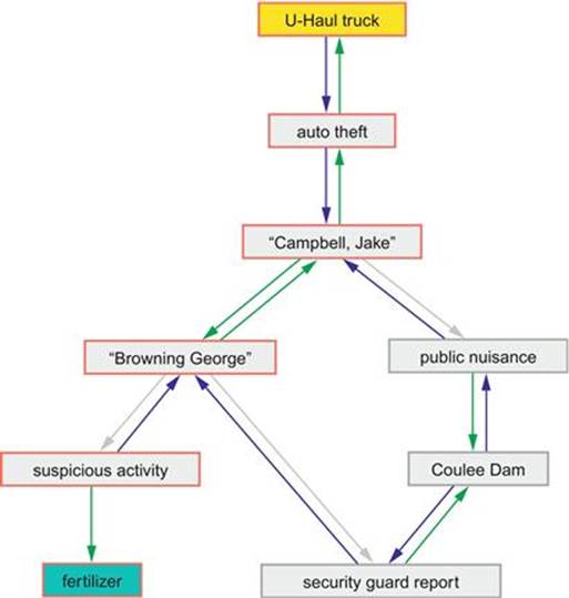
FIGURE 3.1 Possible Terrorist Attack Graph.

In the real world, a major police department has a few hundred cases a week. The super-genius Sherlock Holmes characters are few and far between. But even if you could find such geniuses, you simply do not have enough whiteboards to do this kind of analysis one case at a time in the real world. Intelligence must be computerized in the 21st century if it is going to work.

Most crime is committed by repeat offenders. Repeat offenders tend to follow patterns—some of which are pretty horrible, if you look at serial killers. What a police department wants to do is describe a case, then look through all the open cases to see if there are three or more cases that have the same pattern.

One major advantage is that data goes directly into the graph, while SQL requires that each new fact has to be checked against the existing data. Then the SQL data has to be encoded on some scale to fit into a column with a particular data type.

3.4 Vertex Covering

Social network marketing depends on finding “the cool kids,” the trendsetters who know everybody in a community. In some cases, it might be one person. The Pope is fairly well known among Catholics, for example, and his opinions carry weight.

Formally, a vertex cover of an undirecterd graph G is a set C of vertices such that each edge of G is incident to at least one vertex in C. The set C is said to cover the edges of G. Informally, you have a weird street map and want to put up security cameras at intersections (nodes) in such a way that no street (edge) is not under surveillance. We also talk about coloring the nodes to mark them as members of the set of desired vertices. Figure 3.2 shows two vertex coverings taken from a Wikipedia article on this topic.

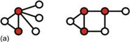
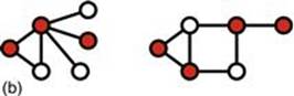
FIGURE 3.2 Vertex coverings from Wikipedia: (a) three-node solution, and (b) a four-node solution.

However, neither of these coverings is minimal. The three-node solution can be reduced to two nodes, and the four-node solution can be reduced to three nodes, as follows:

CREATE TABLE Grid

(v1 SMALLINT NOT NULL CHECK (v1 > 0),

v2 SMALLINT NOT NULL CHECK (v2 > 0),

PRIMARY KEY (v1, v2),

CHECK (v1 < v2),

color SMALLINT DEFAULT 0 NOT NULL CHECK (color > = 0));

INSERT INTO Grid (v1, v2)

VALUES (1, 2), (1, 4), (2, 3), (2, 5), (2, 6);

{1, 2, 6} and {2, 4} are vertex covers. The second is the minimal cover. Can you prove it? In this example, you can use brute force and try all possible coverings. Finding a vertex covering is known to be an NP-complete problem, so brute force is the only sure way. In practice, this is not a good solution because the combinatorial explosion catches up with you sooner than you think.

One approach is to estimate the size of the cover, then pick random sets of that size. You then keep the best candidates, look for common subgraphs, and modify the candidates by adding or removing nodes. Obviously, when you have covered 100% of the edges, you have a winner; it might not be optimal, but it works.

Another consideration is that the problem might start with a known number of nodes. For example, you want to give n sample items to bloggers to publicize your product. You want to gift the bloggers with the largest readership for the gifts, with the least overlap.

3.5 Graph Programming Tools

As of 2012, there are no ANSI or ISO standard graph query languages. We have to depend on proprietary languages or open-source projects. They depend on underlying graph databases, which are also proprietary or open-source projects. Support for some of the open-source projects is available from commercial providers; Neo4j is the most popular product and it went commercial in 2009 after a decade in the open-source world. This has happened in the relational world with PostgreSQL, MySQL, and other products, so we should not be surprised.

There is an ISO standard known as resource description framework (RDF), which is a standard model for data interchange on the Web. It is based on the RDF that extends the linking structure of the Web to use URIs (uniform resource identifiers) to name the relationship between things as well as the two ends of the link (a triple). URIs can be classified as locators (URLs), names (URNs), or both. A uniform resource name (URN) functions like a person’s name, while a uniform resource locator (URL) resembles that person’s street address. In other words, the URN defines an item’s identity, while the URL provides a method for finding it.

The differences are easier to explain with an example. The ISBN uniquely identifies a specific edition of a book, its identity. But to read the book, you need its location: a URL address. A typical URL would be a file path for the electronic book saved on a local hard disk.

Since the Web is a huge graph database, many graph databases build on RDF standards. This also makes it easier to have a distributed graph database that can use existing tools.

3.5.1 Graph Databases

Some graph databases were built on an existing data storage system to get started, but then were moved to custom storage engines. The reason for this is simple: performance. Assume you want to model a simple one-to-many relationship, such as the Kevin Bacon problem. In RDBMS and SQL, there will be a table for the relationship, which will contain a reference to the table with the unique entity and a reference for each row matching to that entity in the many side of the relationship. As the relational tables grow, the time to perform the join increases because you are working with entire sets.

In a graph model, you start at the Kevin Bacon node and traverse the graph looking at the edges with whatever property you want to use (e.g., “was in a movie with”). If there is a node property, you then filter on it (e.g., “this actor is French”). The edges act like very small, local relationship tables, but they give you a traversal and not a join.

A graph database can have ACID transactions. The simplest possible graph is a single node. This would be a record with named values, called properties. In theory, there is no upper limit on the number of properties in a node, but for practical purposes, you will want to distribute the data into multiple nodes, organized with explicit relationships.

3.5.2 Graph Languages

There is no equivalent to SQL in the graph database world. Graph theory was an established branch of mathematics, so the basic terminology and algorithms were well-known were the first products came along. That was an advantage. But graph database had no equivalent to IBM's System R, the research project that defined SEQUEL, which became SQL. Nor has anyone tried to make one language into the ANSI, ISO or other industry standard.

SPARQL

SPARQL (pronounced “sparkle,” a recursive acronym for SPARQL Protocol and RDF Query Language) is a query language for the RDF format. It tries to look a little like SQL by using common keywords and a bit like C with special ASCII characters and lambda calculus. For example:

PREFIX abc: < http://example.com/exampleOntology#>

SELECT ?capital ?country

WHERE {

?x abc:cityname ?capital;

abc:isCapitalOf ?y.

?y abc:countryname ?country;

abc:isInContinent abc:Africa.}

where the ? prefix is a free variable, and : names a source.

SPASQL

SPASQL (pronounced “spackle”) is an extension of the SQL standard, allowing execution of SPARQL queries within SQL statements, typically by treating them as subqueries or function clauses. This also allows SPARQL queries to be issued through “traditional” data access APIs (ODBC, JDBC, OLE DB, ADO.NET, etc.).

Gremlin

Gremlin is an open-source language that is based on traversals of a property graph with a syntax taken from OO and the C programming language family (https://github.com/tinkerpop/gremlin/wiki). There is syntax for directed edges and more complex queries that looks more mathematical than SQL-like. Following is a sample program. Vertexes are numbered and a traversal starts at one of them. The path is then constructed by in–out paths on the 'likes' property:

g = new Neo4jGraph('/tmp/neo4j')

// calculate basic collaborative filtering for vertex 1

m = [:]

g.v(1).out('likes').in('likes').out('likes').groupCount(m)

m.sort{-it.value}

// calculate the primary eigenvector (eigenvector centrality) of a graph

m = [:]; c = 0;

g.V.out.groupCount(m).loop(2){c++ < 1000}

m.sort{-it.value}

Eigenvector centrality is a measure of the influence of a node in a network. It assigns relative scores to all nodes in the network based on the concept that connections to high-scoring nodes contribute more to the score of the node in question than equal connections to low-scoring nodes. It measures the effect of the “cool kids” in your friends list. Google’s PageRank is a variant of the eigenvector centrality measure.

Cypher (NEO4j)

Cypher is a declarative graph query language that is still growing and maturing, which will make SQL programmers comfortable. It is not a weird mix of odd ASCII charterers, but human-readable keywords in the major clauses. Most of the keywords like WHERE andORDER BY are inspired by SQL. Pattern matching borrows expression approaches from SPARQL. The query language is comprised of several distinct clauses:

◆ START: starting points in the graph, obtained via index lookups or by element IDs.

◆ MATCH: the graph pattern to match, bound to the starting points in START.

◆ WHERE: filtering criteria.

◆ RETURN: what to return.

◆ CREATE: creates nodes and relationships.

◆ DELETE: removes nodes, relationships, and properties.

◆ SET: sets values to properties.

◆ FOREACH: performs updating actions once per element in a list.

◆ WITH: divides a query into multiple, distinct parts.

For example, following is a query that finds a user called John in an index and then traverses the graph looking for friends of John’s friends (though not his direct friends) before returning both John and any friends-of-friends who are found:

START john = node:node_auto_index(name = 'John')

MATCH john-[:friend]- > ()-[:friend]- > fof

RETURN john, fof

We start the traversal at the john node. The MATCH clause uses arrows to show the edges that build the friend-of-friend edges into a path. The final clause tells the query what to return.

In the next example, we take a list of users (by node ID) and traverse the graph looking for those other users who have an outgoing friend relationship, returning only those followed users who have a name property starting with S:

START user = node(5,4,1,2,3)

MATCH user-[:friend]- > follower

WHERE follower.name = ~ 'S.*'

RETURN user, follower.name

The WHERE clause is familiar from SQL and other programming languages. It has the usual logical operators of AND, OR, and NOT; comparison operators; simple math; regular expressions; and so forth.

Trends

Go to http://www.graph-database.org/ for PowerPoint shows on various graph language projects. It will be in flux for the next several years, but you will see several trends. The proposed languages are declarative, and are borrowing ideas from SQL and the RDBMS model. For example, GQL (Graph Query Language) has syntax for SUBGRAPH as a graph venison of a derived table. Much like SQL, the graph languages have to send data to external users, but they lack a standard way of handing off the information.

It is probably worth the effort to get an open-source download of a declarative graph query language and get ready to update your resume.

Concluding Thoughts

Graph databases require a change in the mindset from computational data to relationships. If you are going to work with one of these products, then you ought to get math books on graph theory. A short list of good introductory books are listed in the Reference section.

References

1. Celko J. Trees and hierarchies in SQL for smarties. Burlington, MA: Morgan-Kaufmann; 2012.

2. Chartrand G. Introductory graph theory. Mineola, NY: Dover Publications; 1984.

3. Chartrand G, Zhang P. A first course in graph theory. New York: McGraw-Hill; 2004.

4. Gould R. Graph theory. Mineola, NY: Dover Publications; 2004.

5. Trudeau RJ. Introduction to graph theory. Mineola, NY: Dover Publications; 1994.

6. Maier D. Theory of relational databases. Rockville. MD: Computer Science Press; 1983.

7. Wald A. Sequential analysis. Mineola, NY: Dover Publications; 1973.