Beginning Oracle SQL: For Oracle Database 12c, Third Edition (2014)
Chapter 10. Views
This chapter covers views, a very important component of the relational model (see Ted Codd’s rules in Chapter 1). The first section explains the concept of views. The second section discusses how to use the CREATE VIEW command to create views. In the next section, you’ll learn about the various ways you can use views in SQL, in the areas of retrieval, logical data independency, and security.
Then, in Section 10.4, we explore the (im) possibilities of data manipulation via views. How does it work, which are the constraints, and what should we consider? You’ll learn about updatable views, nonupdatable views, and the WITH CHECK OPTION clause of the CREATE VIEWcommand.
Section 10.5 discusses data manipulation via inline views. This name is slightly confusing, because inline views are not “real” views. Rather, they are subqueries in the FROM clause, as discussed in the previous chapter. Data manipulation via inline views allows you to perform various complicated and creative data manipulation operations, which would otherwise be very complex (or impossible) via the underlying base tables.
Section 10.6 covers views and performance. Following that is a section about materialized views. Materialized views are very popular in data warehousing environments, which have relatively high data volumes with mainly read-only access. Materialized views allow you to improve query response times with some form of controlled redundancy.
We then mention global temporary tables briefly , which are used for performance gains in batch jobs, and end by discussing invisible columns. Views that can see the invisible columns come in handy during development.
10.1 What Are Views?
The result of a query is always a table, or more precisely, a derived table. Compared with “real” tables in the database, the result of a query is volatile, but nevertheless, the result is a table. The only thing that is missing for the query result is a name. Essentially, a view is nothing more than a query with a given name. A more precise definition is as follows:
A view is a virtual table with the result of a stored query as its “contents,” which are derived each time you access the view.
The first part of this definition states two things:
· A view is a virtualtable:That is, you can treat a view (in almost all circumstances) as a table in your SQL statements. Every view has a name, and that’s why views are also referred to as named queries. Views have columns, each with a name and a datatype, so you can execute queries against views, and you can manipulate the “contents” of views (with some restrictions) with INSERT, UPDATE, DELETE, and MERGE commands.
· A view is avirtualtable: In reality, when you access a view, it only behaves like a table. Views don’t have any rows; that’s why the view definition says “contents” (within quotation marks). You define views as named queries, which are stored in the data dictionary; that’s why another common term for views is stored queries. Each time you access the “contents” of a view, Oracle DBMS retrieves the view query from the data dictionary and uses that query to produce the virtual table.
Data manipulation on a view sounds counterintuitive; after all, views don’t have any rows. Therefore you cannot create indexes on views either. Nevertheless, views are supposed to behave like tables as much as possible. If you issue data manipulation commands against a view, the DBMS is supposed to translate those commands into corresponding actions against the underlying base tables. Note that some views are not updatable; that’s why Ted Codd’s rule (see Chapter 1) explicitly refers to views being theoretically updatable. We’ll discuss data manipulation via views in Section 10.4 of this chapter.
Views are not only dependent on changes in the contents of the underlying base tables, but also on certain changes in the structure of those tables. For example, a view doesn’t work anymore if you drop or rename columns of the underlying tables that are referenced in the view definition. On the other hand, if you define an index on a column in the underlying table, it may be used by queries against the column via the view.
10.2 View Creation
You can create views with the CREATE VIEW command. Figure 10-1 shows the corresponding syntax diagram.
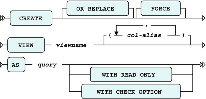
Figure 10-1. A CREATE VIEW syntax diagram
The OR REPLACE option allows you to replace an existing view definition. This is especially useful if you have granted various privileges on your views. View privileges are not retained when you use the DROP VIEW / CREATE VIEW command sequence (as explained later in this section), but a CREATE OR REPLACE VIEW command does preserve them. The FORCE option doesn’t check whether the underlying base tables (used in the view definition) exist or whether you have sufficient privileges to access those base tables. Obviously, these conditions must eventually be met at the time you start using your view definition.
Normally, views inherit their column names from the defining query. However, you should be aware of some possible complications. For example, you might have a query result on your screen showing multiple columns with the same name, and you may have column headings showing functions or other arbitrary column expressions. Obviously, you cannot use query results with these problems as the basis for a view definition. Views have the same column naming rules and constraints as regular tables: column names must be different, and they cannot contain characters such as brackets and arithmetic operators. You can solve such problems in two ways:
· You can specify column aliases in the SELECT clause of the defining query, in such a way that the column headings adhere to all column naming rules and conventions. In this book’s examples, we use this method as much as possible.
· You can specify explicit column aliases in the CREATE VIEW command between the view name and the AS clause (see Figure 10-1).
The WITHCHECK OPTION and WITH READ ONLY options influence view behavior under data manipulation activity, as described later in this chapter, in Section 10-4.
Listing 10-1 shows two very similar SQL statements. However, note the main difference; the first statement creates a view, and the second statement creates a table.
Listing 10-1. Views vs. Tables
SQL> create view dept20_v as
2 select * from employees where deptno = 20;
View created.
SQL> create table dept20_t as
2 select * from employees where deptno = 20;
Table created.
SQL>
The “contents” of the view DEPT20_V will always be fully dependent on the EMPLOYEES table. The table DEPT20_T uses the current EMPLOYEES table as only a starting point. Once created, it is a fully independent table with its own contents.
Creating a View from a Query
Listing 10-2 shows an example of a regular query with its result. The query is a join over three tables, providing information about all employees and their departments. Note that we use an alias in the SELECT clause (see line 6) to make sure that all columns in the query result have different names. See line 2, where you select the ENAME column, too.
Listing 10-2. A Regular Query, Joining Three Tables
SQL> select e.empno
2 , e.ENAME
3 , e.init
4 , d.dname
5 , d.location
6 , m.ENAME as MANAGER
7 from employees e
8 join
9 departments d using (deptno)
10 join
11 employees m on (e.empno = d.mgr);
EMPNO ENAME INIT DNAME LOCATION MANAGER
-------- -------- ----- ---------- -------- -------
7369 SMITH N TRAINING DALLAS JONES
7499 ALLEN JAM SALES CHICAGO BLAKE
7521 WARD TF SALES CHICAGO BLAKE
7566 JONES JM TRAINING DALLAS JONES
7654 MARTIN P SALES CHICAGO BLAKE
7698 BLAKE R SALES CHICAGO BLAKE
7782 CLARK AB ACCOUNTING NEW YORK CLARK
7788 SCOTT SCJ TRAINING DALLAS JONES
7839 KING CC ACCOUNTING NEW YORK CLARK
7844 TURNER JJ SALES CHICAGO BLAKE
7876 ADAMS AA TRAINING DALLAS JONES
7900 JONES R SALES CHICAGO BLAKE
7902 FORD MG TRAINING DALLAS JONES
7934 MILLER TJA ACCOUNTING NEW YORK CLARK
14 rows selected.
SQL>
Listing 10-3 shows how you can transform this query into a view definition, by inserting one additional line at the beginning of the command.
Listing 10-3. Creating a View from the Query in Listing 10-2
SQL> create view empdept_v as -- This line is added
2 select e.empno
3 , e.ENAME
4 , e.init
5 , d.dname
6 , d.location
7 , m.ENAME as MANAGER
8 from employees e
9 join
10 departments d using (deptno)
11 join
12 employees m on (m.empno = d.mgr);
View created.
SQL>
This view is now a permanent part of your collection of database objects. However, note that if we had not used an alias for m.ENAME in line 7, Listing 10-3 would give the following Oracle error message:
ORA-00957: duplicate column name
Getting Information about Views from the Data Dictionary
Listing 10-4 queries the USER_OBJECTS data dictionary view. As you can see, you now have two views in your schema: DEPT20_V and EMPDEPT_V.
Listing 10-4. Querying the Data Dictionary to See Your Views
SQL> select object_name, object_type
2 from user_objects
3 where object_type in ('TABLE','VIEW')
4 order by object_type, object_name;
OBJECT_NAME OBJECT_TYPE
------------------------------ -----------
COURSES TABLE
DEPARTMENTS TABLE
DEPT20_T TABLE
E TABLE
EMPLOYEES TABLE
HISTORY TABLE
OFFERINGS TABLE
REGISTRATIONS TABLE
SALGRADES TABLE
DEPT20_V VIEW
EMPDEPT_V VIEW
11 rows selected.
SQL>
Listing 10-5 shows that you can use the SQL*Plus DESCRIBE command on a view, just as you can on regular tables, and it also shows an example of a query against a view.
Listing 10-5. Using DESCRIBE and Writing Queries Against Views
SQL> describe empdept_v
Name Null? Type
----------------------------- -------- -------------
EMPNO NOT NULL NUMBER(4)
ENAME NOT NULL VARCHAR2(8)
INIT NOT NULL VARCHAR2(5)
DNAME NOT NULL VARCHAR2(10)
LOCATION NOT NULL VARCHAR2(8)
MANAGER NOT NULL VARCHAR2(8)
SQL> select * from empdept_v where manager = 'CLARK';
EMPNO ENAME INIT DNAME LOCATION MANAGER
-------- -------- ----- ---------- -------- --------
7934 MILLER TJA ACCOUNTING NEW YORK CLARK
7839 KING CC ACCOUNTING NEW YORK CLARK
7782 CLARK AB ACCOUNTING NEW YORK CLARK
SQL>
You can query the USER_VIEWS data dictionary view to retrieve your view definitions, as shown in Listing 10-6.
![]() Note The two leading SQL*Plus commands in Listing 10-6 are used only to make the results more readable. Chapter 11 discusses these (and many other) SQL*Plus commands in more detail.
Note The two leading SQL*Plus commands in Listing 10-6 are used only to make the results more readable. Chapter 11 discusses these (and many other) SQL*Plus commands in more detail.
Listing 10-6. Retrieving View Definitions from the Data Dictionary
SQL> set long 999
SQL> column text format a42 word wrapped
SQL> select view_name, text
2 from user_views;
VIEW_NAME TEXT
------------------------------ ------------------------------------------
DEPT20_V select "EMPNO","ENAME","INIT","JOB",
"MGR","BDATE","MSAL","COMM","DEPTNO"
from employees where deptno=20
EMPDEPT_V select e.empno
, e.ENAME
, e.init
, d.dname
, d.location
, m.ENAME as MANAGER
from employees e
join
departments d using (deptno)
join
employees m on (m.empno = d.mgr)
SQL>
Apparently, if you define a view with a query starting with SELECT * FROM ..., the asterisk (*) gets expanded (and stored) as a comma-separated list of column names. Compare the query in Listing 10-1, where you created the DEPT20_V view, with the TEXT column contents inListing 10-6. One might think that by using SELECT * FROM the view will become dynamic and will encompass any future columns added to the underlying table, but that is not the case exactly because the asterisk results in hardcoded column names in the data dictionary saved version of the view.
Replacing and Dropping Views
You cannot change the definition of an existing view. Oracle SQL offers an ALTER VIEW command, but you can use that command only to recompile views that became invalid, which would happen after for instance an alter command on the underlying table. You can drop a view definition only, with the DROP VIEW command.
The DROPVIEW command is very straightforward, and doesn’t need additional explanation:
SQL> drop view <view_name>;
Alternatively, you can replace the definition of an existing view with the CREATEOR REPLACE VIEW command, as described earlier in this section.
10.3 What Can You Do with Views?
You can use views for many different purposes. This section lists and explains the most important ones: to simplify database retrieval, to maintain logical data independence, and to implement data security.
Simplifying Data Retrieval
Views can simplify database retrieval significantly. You can build up (and test) complex queries step by step for more control over the correctness of your queries. In other words, you will be more confident that your queries return the right results.
You can also store (hide) frequently recurring standard queries in a view definition, thus reducing the number of unnecessary mistakes. For example, you might define views based on frequently joined tables, UNION constructs, or complex GROUP BY statements.
Suppose we are interested in an overview showing all employees who have attended more course days than the average employee. This is not a trivial query, so let’s tackle it in multiple phases. As a first step toward the final solution, we ask the question, “How many course days did everyone attend?” The query in Listing 10-7 provides the answer.
Listing 10-7. Working Toward a Solution: Step 1
SQL> select e.empno
2 , e.ename
3 , sum(c.duration) as days
4 from registrations r
5 join courses c on (c.code = r.course)
6 join employees e on (e.empno = r.attendee)
7 group by e.empno
8 , e.ename;
EMPNO ENAME DAYS
-------- -------- --------
7900 JONES 3
7499 ALLEN 11
7521 WARD 1
7566 JONES 5
7698 BLAKE 12
7782 CLARK 4
7788 SCOTT 12
7839 KING 8
7844 TURNER 1
7876 ADAMS 9
7902 FORD 9
7934 MILLER 4
12 rows selected.
SQL>
This is not the solution to our problem yet, but it is already quite complicated. We have a JOIN and a GROUP BY clause over a combination of two columns. If the result in Listing 10-7 were a real table, our original problem would be much easier to solve. Well, we can simulate that situation by defining a view. So we add one extra line to the query in Listing 10-7, as shown in Listing 10-8.
Listing 10-8. Working Toward a Solution: Step 2
SQL> create or replace view course_days as
2 select e.empno
3 , e.ename
4 , sum(c.duration) as days
5 from registrations r
6 join courses c on (c.code = r.course)
7 join employees e on (e.empno = r.attendee)
8 group by e.empno
9 , e.ename;
View created.
SQL> select *
2 from course_days
3 where days > 10;
EMPNO ENAME DAYS
-------- -------- --------
7499 ALLEN 11
7698 BLAKE 12
7788 SCOTT 12
SQL>
Now, the original problem is rather easy to solve. Listing 10-9 shows the solution.
Listing 10-9. Working Toward a Solution: The Final Step
SQL> select *
2 from course_days
3 where days > (select avg(days)
4 from course_days);
EMPNO ENAME DAYS
-------- -------- --------
7499 ALLEN 11
7698 BLAKE 12
7788 SCOTT 12
7839 KING 8
7876 ADAMS 9
7902 FORD 9
SQL>
Of course, you could argue that you could solve this query directly against the two base tables, but it is easy to make a little mistake. Moreover, your solution will probably be difficult to interpret. We could have used an inline view as well, or we could have moved the query in Listing 10-7 into a WITH clause, as described in Section 9.4 of Chapter 9. Inline views and subquery factoring (using the WITH clause) are good alternatives if you don’t have the right system privileges to create views. A big advantage of using views, compared with inline views and subquery factoring, is the fact that view definitions are persistent; that is, you might benefit from the same view for more than one problem. Views occupy very little space (the DBMS stores the query text only), and there is no redundancy at all.
Maintaining Logical Data Independence
You can use views to change the (logical) external interface of the database, as exposed to database users and applications, without the need to change the underlying database structures themselves. In other words, you can use views to implement logical data independency. For example, different database users can have different views on the same base tables. You can rearrange columns, filter on rows, change table and column names, and so on.
Distributed databases often use views (or synonyms) to implement logical data independency and hide complexity. Synonyms are simple pointers, whereas views are (complex) SELECTs with a given name. See Chapter 7 for more about synonyms. For example, you can define (and store) a view as a “local” database object. Behind the scenes, the view query accesses data from other databases on the network, but this is completely transparent to database users and applications.
You can also provide derivable information via views; that is, you implement redundancy at the logical level. The COURSE_DAYS view we created in Listing 10-8 is an example, because that view derives the number of course days.
Implementing Data Security
Last, but not least, views are a powerful means to implement data security. Views allow you to hide certain data from database users and applications. The view query precisely determines which rows and columns are exposed via the view. By using the GRANT and REVOKE commands on your views, you specify in detail which actions against the view data are allowed. In this approach, you don’t grant any privileges at all on the underlying base tables, since you obviously don’t want database users or applications to bypass the views and access the base tables directly.
10.4 Data Manipulation via Views
As you’ve learned in this chapter, views are virtual tables, and they are supposed to behave like tables as much as possible. For retrieval, that’s no problem. However, data manipulation via views is not always possible. A view is theoretically updatable if the DML command against the view can be unambiguously decomposed into corresponding DML commands against rows and columns of the underlying base tables.
Let’s consider the three views created in Listings 10-10 and 10-11.
Listing 10-10. CRS_OFFERINGS View, Based on a Join
SQL> create or replace view crs_offerings as
2 select o.course as course_code, c.description, o.begindate
3 from offerings o
4 join
5 courses c
6 on (o.course = c.code);
View created.
SQL>
Listing 10-11. Simple EMP View and Aggregate AVG_EVALUATIONS View
SQL> create or replace view emp as
2 select empno, ename, init
3 from employees;
View created.
SQL> create or replace view avg_evaluations as
2 select course
3 , avg(evaluation) as avg_eval
4 from registrations
5 group by course;
View created.
SQL>
First, let’s look at the simplest view: the EMP view. The Oracle DBMS should be able to delete rows from the EMPLOYEES table via this view, or to change any of the three column values exposed by the view. However, inserting new rows via this view is impossible, because theEMPLOYEES table has NOT NULL columns without a default value (such as the date of birth) outside the scope of the EMP view. See Listing 10-12 for some DML experiments against the EMP view.
Listing 10-12. Testing DML Commands Against the EMP View
SQL> delete from emp
2 where empno = 7654;
1 row deleted.
SQL> update emp
2 set ename = 'BLACK'
3 where empno = 7698;
1 row updated.
SQL> insert into emp
2 values (7999,'NEWGUY','NN');
insert into e
*
ERROR at line 1:
ORA-01400: cannot insert NULL into ("BOOK"."EMPLOYEES"."BDATE")
SQL> rollback;
Rollback complete.
SQL>
Note that the ORA-01400 error message in Listing 10-12 actually reveals several facts about the underlying (and supposedly hidden) table:
· The schema name (BOOK)
· The table name (EMPLOYEES)
· The presence of a mandatory BDATE column
Before you think you’ve discovered a security breach in the Oracle DBMS, I should explain that you get this informative error message only because you are testing the EMP view while connected as BOOK. If you are connected as a different database user with INSERT privilege against the EMP view only, the error message becomes as follows:
ORA-01400: cannot insert NULL into (???)
Updatable Join Views
The CRS_OFFERINGS view (see Listing 10-10) is based on a join of two tables: OFFERINGS and COURSES. Nevertheless, you are able to perform some data manipulation via this view, as long as the data manipulation can be translated into corresponding actions against the two underlying base tables. CRS_OFFERINGS is an example of an updatable join view. The Oracle DBMS is getting closer and closer to the full implementation of Ted Codd’s rule about views (see Chapter 1). Listing 10-13 demonstrates testing some DML commands against this view.
Listing 10-13. Testing DML Commands Against the CRS_OFFERINGS View
SQL> delete from crs_offerings where course_code = 'ERM';
1 row deleted.
SQL> insert into crs_offerings (course_code, begindate)
2 values ('OAU' , trunc(sysdate));
1 row created.
SQL> rollback;
Rollback complete.
SQL>
There are some rules and restrictions that apply to updatable join views. Also, the concept of key-preserved tables plays an important role in this area. As the name indicates, a key-preserved table is an underlying base table with a one-to-one row relationship with the rows in the view, via the primary key or a unique key.
These are some examples of updatable join view restrictions:
· You are allowed to issue DML commands against updatable join views only if you change a single underlying base table.
· For INSERTstatements, all columns into which values are inserted must belong to a key-preserved table.
· For UPDATEstatements, all columns updated must belong to a key-preserved table.
· For DELETEstatements, if the join results in more than one key-preserved table, the Oracle DBMS deletes from the first table named in the FROM clause.
· If you created the view using WITH CHECK OPTION, some additional DML restrictions apply, as explained a little later in this section.
As you can see in Listing 10-13, the DELETE and INSERT statements against the CRS_OFFERINGS updatable join view succeed. Feel free to experiment with other data manipulation commands. The Oracle error messages are self-explanatory if you hit one of the restrictions:
ORA-01732: data manipulation operation not legal on this view
ORA-01752: cannot delete from view without exactly one key-preserved table
ORA-01779: cannot modify a column which maps to a non key-preserved table
Nonupdatable Views
First of all, if you create a view with the WITH READ ONLY option (see Figure 10-1), data manipulation via that view is impossible by definition, regardless of how you defined the view.
The AVG_EVALUATIONS view definition (see Listing 10-11) contains a GROUP BY clause. This implies that there is no longer a one-to-one relationship between the rows of the view and the rows of the underlying base table. Therefore, data manipulation via the AVG_EVALUATIONSview is impossible.
If you use SELECT DISTINCT in your view definition, this has the same effect: it makes your view nonupdatable. You should try to avoid using SELECT DISTINCT in view definitions, because it has additional disadvantages; for example, each view access will force a sort to take place, whether or not you need it.
The set operators UNION, MINUS, and INTERSECT also result in nonupdatable views. For example, imagine that you are trying to insert a row via a view based on a UNION—in which underlying base table should the DBMS insert that row?
The Oracle documentation provides all of the details and rules with regard to view updatability. Most rules and exceptions are rather straightforward, and as noted earlier, most Oracle error messages clearly indicate the reason why certain data manipulation commands are forbidden.
The data dictionary offers a helpful view to find out which of your view columns are updatable: the USER_UPDATABLE_COLUMNS view. For example, Listing 10-14 shows that you cannot do much with the DESCRIPTION column of the CRS_OFFERINGS view. This is because it is based on a column from the COURSES table, which is not a key-preserved table in this view.
Listing 10-14. View Column Updatability Information from the Data Dictionary
SQL> select column_name
2 , updatable, insertable, deletable
3 from user_updatable_columns
4 where table_name = 'CRS_OFFERINGS';
COLUMN_NAME UPD INS DEL
-------------------- --- --- ---
COURSE_CODE YES YES YES
DESCRIPTION NO NO NO
BEGINDATE YES YES YES
SQL>
MAKING A VIEW UPDATABLE WITH INSTEAD-OF TRIGGERS
In a chapter about views, it’s worth mentioning that PL/SQL (the standard procedural programming language for Oracle databases) provides a way to make any view updatable. With PL/SQL, you can define instead-of triggers on your views. These triggers take over control as soon as any data manipulation commands are executed against the view.
This means that you can make any view updatable, if you choose, by writing some procedural PL/SQL code. Obviously, it is your sole responsibility to make sure that those instead-of triggers do the “right things” to your database to maintain data consistency and integrity. Instead-of triggers should not be your first thought to solve data manipulation issues with views. However, they may solve your problems in some special cases, or they may allow you to implement a very specific application behavior.
The WITH CHECK OPTION Clause
If data manipulation is allowed via a certain view, there are two rather curious situations that deserve attention:
· You change rows with an UPDATE command against the view, and then the rows don’t show up in the view anymore.
· You add rows with an INSERT command against the view; however, the rows don’t show up when you query the view.
Disappearing Updated Rows
Do you still have the DEPT20_V view, created in Listing 10-1? Check out what happens in Listing 10-15: by updating four rows, they disappear from the view.
Listing 10-15. UPDATE Makes Rows Disappear
SQL> select * from dept20_v;
EMPNO ENAME INIT JOB MGR BDATE MSAL COMM DEPTNO
----- -------- ----- -------- ----- ----------- ----- ----- ------
7369 SMITH N TRAINER 7902 17-DEC-1965 800 20
7566 JONES JM MANAGER 7839 02-APR-1967 2975 20
7788 SCOTT SCJ TRAINER 7566 26-NOV-1959 3000 20
7876 ADAMS AA TRAINER 7788 30-DEC-1966 1100 20
7902 FORD MG TRAINER 7566 13-FEB-1959 3000 20
SQL> update dept20_v
2 set deptno = 30
3 where job ='TRAINER';
4 rows updated.
SQL> select * from dept20_v;
EMPNO ENAME INIT JOB MGR BDATE MSAL COMM DEPTNO
----- -------- ----- -------- ----- ----------- ----- ----- ------
7566 JONES JM MANAGER 7839 02-APR-1967 2975 20
SQL> rollback;
Rollback complete.
SQL>
Apparently, the updates in Listing 10-15 are propagated to the underlying EMPLOYEES table. All trainers from department 20 don’t show up anymore in the DEPT20_V view, because their DEPTNO column value is changed from 20 to 30.
Inserting Invisible Rows
The second curious scenario is shown in Listing 10-16. You insert a new row for employee 9999, and you get the message 1 row created. However, the new employee does not show up in the query.
Listing 10-16. INSERT Rows Without Seeing Them in the View
SQL> insert into dept20_v
2 values ( 9999,'BOS','D', null, null
3 , date '1939-01-01'
4 , '10', null, 30);
1 row created.
SQL> select * from dept20_v;
EMPNO ENAME INIT JOB MGR BDATE MSAL COMM DEPTNO
----- -------- ----- -------- ----- ----------- ----- ----- ------
7369 SMITH N TRAINER 7902 17-DEC-1965 800 20
7566 JONES JM MANAGER 7839 02-APR-1967 2975 20
7788 SCOTT SCJ TRAINER 7566 26-NOV-1959 3000 20
7876 ADAMS AA TRAINER 7788 30-DEC-1966 1100 20
7902 FORD MG TRAINER 7566 13-FEB-1959 3000 20
5 rows selected.
SQL> rollback;
Rollback complete.
SQL>
Listing 10-16 shows that you can insert a new employee via the DEPT20_V view into the underlying EMPLOYEES table without the new row showing up in the view itself.
Preventing These Two Scenarios
If the view behavior just described is undesirable, you can create your views with the WITH CHECK OPTION clause (see Figure 10-1). Actually, the syntax diagram in Figure 10-1 is not complete. You can assign a name to WITH CHECK OPTIONconstraints, as follows:
SQL> create [or replace] view ... with check option constraint <cons-name>;
If you don’t provide a constraint name, the Oracle DBMS generates a rather cryptic one for you.
Listing 10-17 replaces the DEPT20_V view, using WITH CHECK OPTION, and shows that the INSERT statement that succeeded in Listing 10-16 now fails with an Oracle error message.
Listing 10-17. Creating Views WITH CHECK OPTION
SQL> create or replace view dept20_v as
2 select * from employees where deptno = 20
3 with check option constraint dept20_v_check;
View created.
SQL> insert into dept20_v
2 values ( 9999,'BOS','D', null, null
3 , date '1939-01-01'
4 , '10', null, 30);
, '10', null, 30)
*
ERROR at line 4:
ORA-01402: view WITH CHECK OPTION where-clause violation
SQL>
Constraint Checking
In the old days, when the Oracle DBMS didn’t yet support referential integrity constraints (which is a long time ago, before Oracle7), you were still able to implement certain integrity constraints by using WITH CHECK OPTION when creating views. For example, you could use subqueries in the view definition to check for row existence in other tables. Listing 10-18 gives an example of such a view. Nowadays, you don’t need this technique anymore, of course.
Listing 10-18. WITH CHECK OPTION and Constraint Checking
SQL> create or replace view reg_view as
2 select r.*
3 from registrations r
4 where r.attendee in (select empno
5 from employees)
6 and r.course in (select code
7 from courses 8 and r.evaluation in (1,2,3,4,5)
9 with check option;
View created.
SQL> select constraint_name, table_name
2 from user_constraints
3 where constraint_type = 'V';
CONSTRAINT_NAME TABLE_NAME
-------------------- --------------------
SYS_C005979 REG_VIEW
DEPT20_V_CHECK DEPT20_V
SQL>
Via the REG_VIEW view, you can insert registrations only for an existing employee and an existing course. Moreover, the EVALUATION value must be an integer between 1 and 5, or a null value. Any data manipulation command against the REG_VIEW view that violates one of the above three checks will result in an Oracle error message. CHECK OPTION constraints show up in the data dictionary with a CONSTRAINT_TYPE value V; notice the system generated constraint name for theREG_VIEW view.
10.5 Data Manipulation via Inline Views
Inline views are subqueries assuming the role of a table expression in SQL commands. In other words, you specify a subquery (between parentheses) in places where you would normally specify a table or view name. We already discussed inline views in the previous chapter, but we considered inline views only in the FROM component of queries.
You can also use inline views for data manipulation purposes. Data manipulation via inline views is especially interesting in combination with updatable join views. Listing 10-19 shows an example of an UPDATE command against an inline updatable join view.
Listing 10-19. UPDATE via an Inline Updatable Join View
SQL> update ( select e.msal
2 from employees e join
3 departments d using (deptno)
4 where location = 'DALLAS')
5 set msal = msal + 1;
5 rows updated.
SQL> rollback;
Rollback complete.
SQL>
Listing 10-19 shows that you can execute UPDATE commands via an inline join view, giving all employees in Dallas a symbolic salary raise. Note that the UPDATE command does not contain a WHERE clause at all; the inline view filters the rows to be updated. This filtering would be rather complicated to achieve in a regular UPDATE command against the EMPLOYEES table. For that, you probably would need a correlated subquery in the WHERE clause.
At first sight, it may seem strange to perform data manipulation via inline views (or subqueries), but the number of possibilities is almost unlimited. The syntax is elegant and readable, and the response time is at least the same (if not better) compared with the corresponding commands against the underlying base tables. Obviously, all restrictions regarding data manipulation via updatable join views (as discussed earlier in this section) still apply.
10.6 Views and Performance
Normally, the Oracle DBMS processes queries against views in the following way:
1. The DBMS notices that views are involved in the query entered.
2. The DBMS retrieves the view definition from the data dictionary.
3. The DBMS merges the view definition with the query entered.
4. The optimizer chooses an appropriate execution plan for the result of the previous step: a command against base tables.
5. The DBMS executes the plan from the previous step.
In exceptional cases, the Oracle DBMS may decide to execute the view query from the data dictionary, populate a temporary table with the results, and then use the temporary table as a base table for the query entered. This happens only if the Oracle DBMS is not able to merge the view definition with the query entered, or if the Oracle optimizer determines that using a temporary table is a good idea.
In the regular approach, as outlined in the preceding five steps, steps 2 and 3 are the only additional overhead. One of the main advantages of this approach is that you can benefit optimally from indexes on the underlying base tables.
For example, suppose you enter the following query against the AVG_EVALUATIONS view:
SQL> select *
2 from avg_evaluations
3 where avg_eval >= 4
This query is transformed internally into the statement shown in Listing 10-20. Notice that the WHERE clause is translated into a HAVING clause, and the asterisk (*) in the SELECT clause is expanded to the appropriate list of column expressions.
Listing 10-20. Rewritten Query Against the REGISTRATIONS Table
SQL> select r.course
2 , avg(r.evaluation) as avg_eval
3 from registrations r
4 group by r.course
5 having avg(r.evaluation) >= 4;
COURSE AVG_EVAL
------ --------
JAV 4.125
OAU 4.5
XML 4.5
SQL>
Especially when dealing with larger tables, the performance overhead of using views is normally negligible. If you start defining views on views on views, the performance overhead may become more significant. And, in case you don’t trust the performance overhead, you can always use diagnostic tools such as SQL *Plus or SQL Developer AUTOTRACE (see Chapter 7, Section 7.6) to check execution plans and statistics.
Complex views with many columns joined from several tables are sometimes misused for choosing data from just one of those tables—in which case, the performance will not be impressive. But then again, it might be the only choice when lacking privileges on the underlying tables.
10.7 Materialized Views
A brief introduction of materialized views makes sense in this chapter about views. The intent of this section is to illustrate the concept of materialized views using a simple example.
Normally, materialized views are mainly used in complex data warehousing environments, where the tables grow so big that the data volume causes unacceptable performance problems. An important property of data warehousing environments is that you don’t change the data very often. Typically, there is a separate Extraction, Transformation, Loading (ETL) process that updates the data warehouse contents.
Materialized views are also often used with distributed databases. In such environments, accessing data over the network can become a performance bottleneck. You can use materialized views to replicate data in a distributed database.
To explore materialized views, let’s revisit Listing 10-1 and add a third DDL command, as shown in Listing 10-21.
Listing 10-21. Comparing Views, Tables, and Materialized Views
SQL> create or replace VIEW dept20_v as
2 select * from employees where deptno = 20;
View created.
SQL> create TABLE dept20_t as
2 select * from employees where deptno = 20;
Table created.
SQL> create MATERIALIZED VIEW dept20_mv enable query rewrite as
2 select * from employees where deptno = 20;
Materialized view created.
SQL>
You already know the difference between a table and a view, but what is a materialized view? Well, as the name suggests, it’s a view for which you store both its definition and the query results. In other words, a materialized view has its own rows. Materialized views imply redundant data storage.
The materialized view DEPT20_MV now contains all employees of department 20, and you can execute queries directly against DEPT20_MV, if you like. However, that’s not the main purpose of creating materialized views, as you will learn from the remainder of this section.
Properties of Materialized Views
Materialized views have two important properties in the areas of maintenance and usage:
· Maintenance: Materialized views are “snapshots.” That is, they have a certain content at any point in time, based on “refreshment” from the underlying base tables. This implies that the contents of materialized views are not necessarily up-to-date all the time, because the underlying base tables can change. Fortunately, the Oracle DBMS offers various features to automate the refreshment of your materialized views completely, in an efficient way. In other words, yes, you have redundancy, but you can easily set up appropriate redundancy control.
· Usage: The Oracle optimizer (the component of the Oracle DBMS deciding about execution plans for SQL commands) is aware of the existence of materialized views. The optimizer also knows whether materialized views are up-to-date or stale. The optimizer can use this knowledge to replace queries written against regular base tables with corresponding queries against materialized views, if the optimizer thinks that approach may result in better response times. This is referred to as the query rewrite feature, which is explained in the next section.
![]() Note When you create materialized views, you normally specify whether you want to enable query rewrite, and how you want the Oracle DBMS to handle the refreshing of the materialized view. Those syntax details are used in Listing 10-21 but further usage information is omitted here. See Oracle SQL Reference for more information.
Note When you create materialized views, you normally specify whether you want to enable query rewrite, and how you want the Oracle DBMS to handle the refreshing of the materialized view. Those syntax details are used in Listing 10-21 but further usage information is omitted here. See Oracle SQL Reference for more information.
Query Rewrite
Let’s continue with our simple materialized view, created in Listing 10-21. Assume you enter the following query, selecting all trainers from department 20:
SQL> select * from employees where deptno = 20 and job = 'TRAINER'
For this query, the optimizer may decide to execute the following query instead:
SQL> select * from dept20_mv where job = 'TRAINER'
In other words, the original query against the EMPLOYEES table is rewritten against the DEPT20_MV materialized view. Because the materialized view contains fewer rows than the EMPLOYEES table (and therefore fewer rows need to be scanned), the optimizer thinks it is a better starting point to produce the desired end result. Listing 10-22 shows query rewrite at work using the SQL*Plus AUTOTRACE feature.
Listing 10-22. Materialized Views and Query Rewrite at Work
SQL> set autotrace on explain
SQL> select * from employees where deptno = 20 and job = 'TRAINER';
EMPNO ENAME INIT JOB MGR BDATE MSAL COMM DEPTNO
------ -------- ----- -------- ----- ----------- ----- ----- ------
7369 SMITH N TRAINER 7902 17-DEC-1965 800 20
7788 SCOTT SCJ TRAINER 7566 26-NOV-1959 3000 20
7876 ADAMS AA TRAINER 7788 30-DEC-1966 1100 20
7902 FORD MG TRAINER 7566 13-FEB-1959 3000 20
Execution Plan
----------------------------------------------------------
Plan hash value: 2578977254
------------------------------------------------------------------------------------------
| Id | Operation | Name | Rows | Bytes | Cost (%CPU)| Time |
------------------------------------------------------------------------------------------
| 0 | SELECT STATEMENT | | 4 | 360 | 3 (0)| 00:00:01 |
|* 1 | MAT_VIEW REWRITE ACCESS FULL| DEPT20_MV | 4 | 360 | 3 (0)| 00:00:01 |
------------------------------------------------------------------------------------------
Predicate Information (identified by operation id):
---------------------------------------------------
1 - filter("DEPT20_MV"."JOB"='TRAINER')
SQL>
Although it is obvious from Listing 10-22 that you write a query against the EMPLOYEES table, the execution plan (produced with AUTOTRACE ON EXPLAIN) shows that the materialized view DEPT20_MV is accessed instead.
Materialized views normally provide better response times; however, there is a risk that the results are based on stale data because the materialized views are out of sync with the underlying base tables. You can specify whether you tolerate query rewrites in such cases, thus controlling the behavior of the optimizer. If you want precise results, the optimizer considers query rewrite only when the materialized views are guaranteed to be up-to-date.
Obviously, the materialized view example we used in this section is much too simple. Normally, you create materialized views with relatively “expensive” operations, such as aggregation (GROUP BY), joins over multiple tables, and set operators (UNION, MINUS, and INTERSECT)—operations that are too time-consuming to be repeated over and over again. For more details and examples of materialized views, see Data Warehousing Guide.
10.8 Global Temporary Table
Another structure that can hold a query result is a global temporary table (GTT), which come in handy for instance in batch jobs.
In your session you may choose to keep some data in a table that you will first populate by doing a complex query against joined tables, then update the interim result a few times, then query into several different reports, and finally you drop the table.
Since you want to update, a view is seldomly an option. Since you end up by dropping the data, an ordinary table or a materialized view are unnecessarily permanent objects, and so we have Global Temporary Tables. Data in a GTT may last until the end of the transaction or until the end of the session. Notice in the syntax DELETE for transaction life time and PRESERVE for session life time.
CREATE GLOBAL TEMPORARY TABLE <table_name>
(column specifications....)
ON COMMIT { DELETE | PRESERVE } ROWS;
When you commit (or rollback to end the transaction) or exit the session, the data is removed, but the table definition remains in the data dictionary. Several concurrent sessions may use the same GTT since the data is owned exclusively by each session. Performance is better in a GTT exactly because the rows exclusively belong to your session and so need much less locking.
10.9 Invisible Columns
You may be planning for more columns in the next version of your application, but you don’t want them to appear yet in SELECT * queries or to risk that INSERT INTO t VALUES... gets an error, so you make the columns INVISIBLE. For exactly this reason, we advise against usingSELECT * as well as INSERT INTO... without the column list, so use explicit column selection and INSERT INTO t (x,y) VALUES (1,2), that is, with the column list before VALUES.
Let’s make an example table with an invisible column:
SQL> create table t (x number, y number);
Table created.
SQL> alter table t add (newcol number INVISIBLE);
Table altered.
SQL> insert into t (x,y,newcol) values (1,2,3);
1 row created.
When addressing the column explicitly you of course see it.
SQL> select x, y, newcol from t;
X Y NEWCOL
---------- ---------- ----------
1 2 3
With SELECT * you don’t see the column.
SQL> select * from t;
X Y
---------- ----------
1 2
The new thing in 12c is that you can define a view where the column is visible, so you can address it more easily while testing it during development. Columns in views are visible regardless of their visibility in the base table.
SQL> create or replace view see_all as select x,y,newcol from t;
View created.
If we had specified SELECT * while creating the view, the invisible column from table t would never have made it to the view. The CREATE VIEW command hardcodes the columns it finds and explicitly lists them in the saved view text. Since we explicitly selected the newcol, it is part of the view see_all:
SQL> select * from see_all;
X Y NEWCOL
---------- ---------- ----------
1 2 3
In 12c it is possible to make the column INVISIBLE even in the view, if that, for some reason, is your wish. Normally the reason for making the view on top of a table with INVISIBLE columns would be to SEE them, but here is the syntax for making the column invisible even in the view.
SQL> create view see_all
2 (x, y, newcol INVISIBLE)
3 as select x, y, newcol from t;
View created.
10.10 Exercises
As in the previous chapters, we end this chapter with some practical exercises. See Appendix B for the answers.
1. Look at the example discussed in Listings 10-7, 10-8, and 10-9. Rewrite the query in Listing 10-9 without using a view by using the WITH operator.
2. Look at Listing 10-12. How is it possible that you can delete employee 7654 via this EMP view? There are rows in the HISTORY table referring to that employee via a foreign key constraint.
3. Look at the view definition in Listing 10-18. Does this view implement the foreign key constraints from the REGISTRATIONS table to the EMPLOYEES and COURSES tables? Explain your answer.
4. Create a SAL_HISTORY view providing the following overview for all employees based on the HISTORY table: for each employee, show the hire date, the review dates, and the salary changes as a consequence of those reviews. Check your view against the following result:
SQL> select * from sal_history;
EMPNO HIREDATE REVIEWDATE SALARY_RAISE
----- ----------- ----------- ------------
7369 01-JAN-2000 01-JAN-2000
7369 01-JAN-2000 01-FEB-2000 -150
7499 01-JUN-1988 01-JUN-1988
7499 01-JUN-1988 01-JUL-1989 300
7499 01-JUN-1988 01-DEC-1993 200
7499 01-JUN-1988 01-OCT-1995 200
7499 01-JUN-1988 01-NOV-1999 -100
...
7934 01-FEB-1998 01-FEB-1998
7934 01-FEB-1998 01-MAY-1998 5
7934 01-FEB-1998 01-FEB-1999 10
7934 01-FEB-1998 01-JAN-2000 10
79 rows selected.
SQL>
All materials on the site are licensed Creative Commons Attribution-Sharealike 3.0 Unported CC BY-SA 3.0 & GNU Free Documentation License (GFDL)
If you are the copyright holder of any material contained on our site and intend to remove it, please contact our site administrator for approval.
© 2016-2026 All site design rights belong to S.Y.A.