Oracle PL/SQL Programming (2014)

Part V. PL/SQL Application Construction

Chapter 21. Optimizing PL/SQL Performance

Optimizing the performance of an Oracle application is a complex process: you need to tune the SQL in your code base, make sure the system global area (SGA) is properly configured, optimize algorithmic logic, and so on. Tuning individual PL/SQL programs is a bit less daunting, but still more than enough of a challenge. Before spending lots of time changing your PL/SQL code in the hopes of improving the performance of that code, you should:

Tune access to code and data in the SGA

Before your code can be executed (and perhaps run too slowly), it must be loaded into the SGA of the Oracle instance. This process can benefit from a focused tuning effort, usually performed by a DBA. You will find more information about the SGA and other aspects of the PL/SQL architecture in Chapter 24.

Optimize your SQL

In virtually any application you write against the Oracle database, you will do the vast majority of tuning by optimizing the SQL statements executed against your data. The potential inefficiencies of a 16-way join dwarf the usual issues found in a procedural block of code. To put it another way, if you have a program that runs in 20 hours, and you need to reduce its elapsed time to 30 minutes, virtually your only hope will be to concentrate on the SQL within your code. There are many third-party tools available to both DBAs and developers that perform very sophisticated analyses of SQL within applications and recommend more efficient alternatives.

Use the most aggressive compiler optimization level possible

Oracle Database 10g introduced an optimizing compiler for PL/SQL programs. The default optimization level of 2 in that release took the most aggressive approach possible in terms of transforming your code to make it run faster. (Oracle Database 11g and later support an even higher optimization level of 3. The default optimization level, however, is still 2, and that will be sufficient for the vast majority of your code.) You should use this default level unless compilation time is unacceptably slow and you are not seeing benefits from optimization.

Once you are confident that the context in which your PL/SQL code runs is not obviously inefficient, you should turn your attention to your packages and other code. I suggest the following steps:

1. Write your application with best practices and standards in mind.

While you shouldn’t take clearly inefficient approaches to meeting requirements, you also shouldn’t obsess about the performance implications of every line in your code. Remember that most of the code you write will never be a bottleneck in your application’s performance, so optimizing it will not result in any user benefits. Instead, write the application with correctness and maintainability foremost in mind and then...

2. Analyze your application’s execution profile.

Does it run quickly enough? If it does, great: you don’t need to do any tuning (at the moment). If it’s too slow, identify which specific elements of the application are causing the problem and then focus directly on those programs (or parts of programs). Once identified, you can then...

3. Tune your algorithms.

As a procedural language, PL/SQL is often used to implement complex formulas and algorithms. You can use conditional statements, loops, perhaps even GOTOs, and (I hope) reusable modules to get the job done. These algorithms can be written in many different ways, some of which perform very badly. How do you tune poorly written algorithms? This is a tough question with no easy answers. Tuning algorithms is much more complex than tuning SQL (which is “structured” and therefore lends itself more easily to automated analysis).

4. Take advantage of any PL/SQL-specific performance features.

Over the years, Oracle has added statements and optimizations that can make a substantial difference to the execution of your code. Consider using constructs ranging from the RETURNING clause to FORALL. Make sure you aren’t living in the past and paying the price in application inefficiencies.

5. Balance performance improvements against memory consumption.

A number of the techniques that improve the performance of your code also consume more memory, usually in the program global area (PGA), but also sometimes in the SGA. It won’t do you much good to make your program blazingly fast if the resulting memory consumption is unacceptable in your application environment.

It’s outside the scope of this book to offer substantial advice on SQL tuning and database/SGA configuration. I certainly can, on the other hand, tell you all about the most important performance optimization features of PL/SQL, and offer advice on how to apply those features to achieve the fastest PL/SQL code possible.

Finally, remember that overall performance optimization is a team effort. Work closely with your DBA, especially as you begin to leverage key features like collections, table functions, and the function result cache.

Tools to Assist in Optimization

In this section, I introduce the tools and techniques that can help optimize the performance of your code. These fall into several categories: analyzing memory usage, identifying bottlenecks in PL/SQL code, calculating elapsed time, choosing the fastest program, avoiding infinite loops, and using performance-related warnings.

Analyzing Memory Usage

As I mentioned, as you go about optimizing code performance, you will also need to take into account the amount of memory your program consumes. Program data consumes PGA, and each session connected to the Oracle database has its own PGA. Thus, the total memory required for your application is usually far greater than the memory needed for a single instance of the program. Memory consumption is an especially critical factor whenever you work with collections (array-like structures), as well as object types with a large number of attributes and records having a large number of fields.

For an in-depth discussion of this topic, check out the section PL/SQL and Database Instance Memory.

Identifying Bottlenecks in PL/SQL Code

Before you can tune your application, you need to figure out what is running slowly and where you should focus your efforts. Oracle and third-party vendors offer a variety of products to help you do this; generally they focus on analyzing the SQL statements in your code, offering alternative implementations, and so on. These tools are very powerful, yet they can also be very frustrating to PL/SQL developers. They tend to offer an overwhelming amount of performance data without telling you what you really want to know: where are the bottlenecks in your code?

To answer these questions, Oracle offers a number of built-in utilities. Here are the most useful:

DBMS_PROFILER

This built-in package allows you to turn on execution profiling in a session. Then, when you run your code, the Oracle database uses tables to keep track of detailed information about how long each line in your code took to execute. You can then run queries on these tables or—preferably—use screens in products like Toad or SQL Navigator to present the data in a clear, graphical fashion.

DBMS_HPROF (hierarchical profiler)

Oracle Database 11g introduced a hierarchical profiler that makes it easier to roll performance results up through the execution call stack. DBMS_PROFILER provides “flat” data about performance, which makes it difficult to answer questions like “How much time altogether is spent in the ADD_ITEM procedure?” The hierarchical profiler makes it easy to answer such questions.

DBMS_PROFILER

In case you do not have access to a tool that offers an interface to DBMS_PROFILER, here are some instructions and examples.

First of all, Oracle may not have installed DBMS_PROFILER for you automatically. To see if DBMS_PROFILER is installed and available, connect to your schema in SQL*Plus and issue this command:

DESC DBMS_PROFILER

If you then see the message:

ERROR:

ORA-04043: object dbms_profiler does not exist

then you (or your DBA) will have to install the program. To do this, run the $ORACLE_HOME/rdbms/admin/profload.sql file under a SYSDBA account.

You next need to run the $ORACLE_HOME/rdbms/admin/proftab.sql file in your own schema to create three tables populated by DBMS_PROFILER:

PLSQL_PROFILER_RUNS

Parent table of runs

PLSQL_PROFILER_UNITS

Program units executed in run

PLSQL_PROFILER_DATA

Profiling data for each line in a program unit

Once all these objects are defined, you gather profiling information for your application by writing code like this:

BEGIN

DBMS_PROFILER.start_profiler (

'my application' || TO_CHAR (SYSDATE, 'YYYYMMDD HH24:MI:SS')

);

my_application_code;

DBMS_PROFILER.stop_profiler;

END;

Once you have finished running your application code, you can run queries against the data in the PLSQL_PROFILER_ tables. Here is an example of such a query that displays those lines of code that consumed at least 1% of the total time of the run:

/* File on web: slowest.sql */

SELECT TO_CHAR (p1.total_time / 10000000, '99999999')

|| '-'

|| TO_CHAR (p1.total_occur)

AS time_count,

SUBSTR (p2.unit_owner, 1, 20)

|| '.'

|| DECODE (p2.unit_name,

'', '<anonymous>',

SUBSTR (p2.unit_name, 1, 20))

AS unit,

TO_CHAR (p1.line#) || '-' || p3.text text

FROM plsql_profiler_data p1,

plsql_profiler_units p2,

all_source p3,

(SELECT SUM (total_time) AS grand_total

FROM plsql_profiler_units) p4

WHERE p2.unit_owner NOT IN ('SYS', 'SYSTEM')

AND p1.runid = &&firstparm

AND (p1.total_time >= p4.grand_total / 100)

AND p1.runid = p2.runid

AND p2.unit_number = p1.unit_number

AND p3.TYPE = 'PACKAGE BODY'

AND p3.owner = p2.unit_owner

AND p3.line = p1.line#

AND p3.name = p2.unit_name

ORDER BY p1.total_time DESC

As you can see, these queries are fairly complex (I modified one of the canned queries from Oracle to produce the preceding four-way join). That’s why it is far better to rely on a graphical interface in a PL/SQL development tool.

The hierarchical profiler

Oracle Database 11g introduced a second profiling mechanism: DBMS_HPROF, known as the hierarchical profiler. Use this profiler to obtain the execution profile of PL/SQL code, organized by the distinct subprogram calls in your application. “OK,” I can hear you thinking, “but doesn’t DBMS_PROFILER do that for me already?” Not really. Nonhierarchical (flat) profilers like DBMS_PROFILER record the time that your application spends within each subprogram, down to the execution time of each individual line of code. That’s helpful, but in a limited way. Often, you also want to know how much time the application spends within a particular subprogram—that is, you need to “roll up” profile information to the subprogram level. That’s what the new hierarchical profiler does for you.

The PL/SQL hierarchical profiler reports performance information about each subprogram in your application that is profiled, keeping SQL and PL/SQL execution times distinct. The profiler tracks a wide variety of information, including the number of calls to the subprogram, the amount of time spent in that subprogram, the time spent in the subprogram’s subtree (that is, in its descendent subprograms), and detailed parent-child information.

The hierarchical profiler has two components:

Data collector

Provides APIs that turn hierarchical profiling on and off. The PL/SQL runtime engine writes the “raw” profiler output to the specified file.

Analyzer

Processes the raw profiler output and stores the results in hierarchical profiler tables, which can then be queried to display profiler information.

To use the hierarchical profiler, do the following:

1. Make sure that you can execute the DBMS_HPROF package.

2. Make sure that you have WRITE privileges on the directory that you specify when you call DBMS_HPROF.START_PROFILING.

3. Create the three profiler tables (see details on this step below).

4. Call the DBMS_HPROF.START_PROFILING procedure to start the hierarchical profiler’s data collection in your session.

5. Run your application code long and repetitively enough to obtain sufficient code coverage to get interesting results.

6. Call the DBMS_HPROF.STOP_PROFILING procedure to terminate the gathering of profile data.

7. Analyze the contents and then run queries against the profiler tables to obtain results.

NOTE

To get the most accurate measurements of elapsed time for your subprograms, you should minimize any unrelated activity on the system on which your application is running.

Of course, on a production system other processes may slow down your program. You may also want to run these measurements while using real application testing (RAT) in Oracle Database 11g and later to obtain real response times.

To create the profiler tables and other necessary database objects, run the dbmshptab.sql script (located in the $ORACLE_HOME/rdbms/admin directory). This script will create these three tables:

DBMSHP_RUNS

Top-level information about each run of the ANALYZE utility of DBMS_HPROF.

DBMSHP_FUNCTION_INFO

Detailed information about the execution of each subprogram profiled in a particular run of the ANALYZE utility.

DBMSHP_PARENT_CHILD_INFO

Parent-child information for each subprogram profiled in DBMSHP_FUNCTION_INFO.

Here’s a very simple example: I want to test the performance of my intab procedure (which displays the contents of the specified table using DBMS_SQL). So first I start profiling, specifying that I want the raw profiler data to be written to the intab_trace.txt file in the TEMP_DIR directory. This directory must have been previously defined with the CREATE DIRECTORY statement:

EXEC DBMS_HPROF.start_profiling ('TEMP_DIR', 'intab_trace.txt')

Then I call my program (run my application code):

EXEC intab ('DEPARTMENTS')

And then I terminate my profiling session:

EXEC DBMS_HPROF.stop_profiling;

I could have included all three statements in the same block of code; instead, I kept them separate because in most situations you are not going to include profiling commands in or near your application code.

So now that trace file is populated with data. I could open it and look at the data, and perhaps make a little bit of sense of what I find there. A much better use of my time and Oracle’s technology, however, would be to call the ANALYZE utility of DBMS_HPROF. This function takes the contents of the trace file, transforms this data, and places it into the three profiler tables. It returns a run number, which I must then use when querying the contents of these tables. I call ANALYZE as follows:

BEGIN

DBMS_OUTPUT.PUT_LINE (

DBMS_HPROF.ANALYZE ('TEMP_DIR', 'intab_trace.txt'));

END;

/

And that’s it! The data has been collected and analyzed into the tables, and now I can choose from one of two approaches to obtaining the profile information:

1. Run the plshprof command-line utility (located in the directory $ORACLE_HOME/bin/). This utility generates simple HTML reports from either one or two raw profiler output files. For an example of a raw profiler output file, see the section titled “Collecting Profile Data” in theOracle Database Development Guide. I can then peruse the generated HTML reports in the browser of my choice.

2. Run my own “home-grown” queries. Suppose, for example, that the previous block returns 177 as the run number. First, here’s a query that shows all current runs:

3. SELECT runid, run_timestamp, total_elapsed_time, run_comment

FROM dbmshp_runs

Here’s a query that shows me all the names of subprograms that have been profiled, across all runs:

SELECT symbolid, owner, module, type, function, line#, namespace

FROM dbmshp_function_info

Here’s a query that shows me information about subprogram execution for this specific run:

SELECT FUNCTION, line#, namespace, subtree_elapsed_time

, function_elapsed_time, calls

FROM dbmshp_function_info

WHERE runid = 177

This query retrieves parent-child information for the current run, but not in a very interesting way, since I see only key values and not names of programs:

SELECT parentsymid, childsymid, subtree_elapsed_time, function_elapsed_time

, calls

FROM dbmshp_parent_child_info

WHERE runid = 177

Here’s a more useful query, joining with the function information table; now I can see the names of the parent and child programs, along with the elapsed time and number of calls.

SELECT RPAD (' ', LEVEL * 2, ' ') || fi.owner || '.' || fi.module AS NAME

, fi.FUNCTION, pci.subtree_elapsed_time, pci.function_elapsed_time

, pci.calls

FROM dbmshp_parent_child_info pci JOIN dbmshp_function_info fi

ON pci.runid = fi.runid AND pci.childsymid = fi.symbolid

WHERE pci.runid = 177

CONNECT BY PRIOR childsymid = parentsymid

START WITH pci.parentsymid = 1

The hierarchical profiler is a very powerful and rich utility. I suggest that you read Chapter 13 of the Oracle Database Development Guide for extensive coverage of this profiler.

Calculating Elapsed Time

So you’ve found the bottleneck in your application; it’s a function named CALC_TOTALS, and it contains a complex algorithm that clearly needs some tuning. You work on the function for a little while, and now you want to know if it’s faster. You certainly could profile execution of your entire application again, but it would be much easier if you could simply run the original and modified versions “side by side” and see which is faster. To do this, you need a utility that computes the elapsed time of individual programs, even lines of code within a program.

The DBMS_UTILITY package offers two functions to help you obtain this information: DBMS_UTILITY.GET_TIME and DBMS_UTILITY.GET_CPU_TIME. Both are available for Oracle Database 10g and later.

You can easily use these functions to calculate the elapsed time (total and CPU, respectively) of your code down to the hundredth of a second. Here’s the basic idea:

1. Call DBMS_UTILITY.GET_TIME (or GET_CPU_TIME) before you execute your code. Store this “start time.”

2. Run the code whose performance you want to measure.

3. Call DBMS_UTILITY.GET_TIME (or GET_CPU_TIME) to get the “end time.” Subtract start from end; this difference is the number of hundredths of seconds that have elapsed between the start and end times.

Here is an example of this flow:

DECLARE

l_start_time PLS_INTEGER;

BEGIN

l_start_time := DBMS_UTILITY.get_time;

my_program;

DBMS_OUTPUT.put_line (

'Elapsed: ' || DBMS_UTILITY.get_time - l_start_time);

END;

Now, here’s something strange: I find these functions extremely useful, but I never (or rarely) call them directly in my performance scripts. Instead, I choose to encapsulate or hide the use of these functions—and their related “end – start” formula—inside a package or object type. In other words, when I want to test my_program, I would write the following:

BEGIN

sf_timer.start_timer ();

my_program;

sf_timer.show_elapsed_time ('Ran my_program');

END;

I capture the start time, run the code, and show the elapsed time.

I avoid direct calls to DBMS_UTILITY.GET_TIME, and instead use the SFTK timer package, sf_timer, for two reasons:

§ To improve productivity. Who wants to declare those local variables, write all the code to call that mouthful of a built-in function, and do the math? I’d much rather have my utility do it for me.

§ To get consistent results. If you rely on the simple “end – start” formula, you can sometimes end up with a negative elapsed time. Now, I don’t care how fast your code is; you can’t possibly go backward in time!

How is it possible to obtain a negative elapsed time? The number returned by DBMS_UTILITY.GET_TIME represents the total number of seconds elapsed since an arbitrary point in time. When this number gets very big (the limit depends on your operating system), it rolls over to 0 and starts counting again. So if you happen to call GET_TIME right before the rollover, end – start will come out negative!

What you really need to do to avoid the possible negative timing is to write code like this:

DECLARE

c_big_number NUMBER := POWER (2, 32);

l_start_time PLS_INTEGER;

BEGIN

l_start_time := DBMS_UTILITY.get_time;

my_program;

DBMS_OUTPUT.put_line (

'Elapsed: '

|| TO_CHAR (MOD (DBMS_UTILITY.get_time - l_start_time + c_big_number

, c_big_number)));

END;

Who in her right mind, and with the deadlines we all face, would want to write such code every time she needs to calculate elapsed time?

So instead I created the sf_timer package, to hide these details and make it easier to analyze and compare elapsed times.

Choosing the Fastest Program

You’d think that choosing the fastest program would be clear and unambiguous. You run a script, you see which of your various implementations runs the fastest, and you go with that one. Ah, but under what scenario did you run those implementations? Just because you verified top speed for implementation C for one set of circumstances, that doesn’t mean that program will always (or even mostly) run faster than the other implementations.

When testing performance, and especially when you need to choose among different implementations of the same requirements, you should consider and test all the following scenarios:

Positive results

The program was given valid inputs and did what it was supposed to do.

Negative results

The program was given invalid inputs (for example, a nonexistent primary key) and the program was not able to perform the requested tasks.

The data neutrality of your algorithms

Your program works really well against a table of 10 rows, but what about for 10,000 rows? Your program scans a collection for matching data, but what if the matching row is at the beginning, middle, or end of the collection?

Multiuser execution of program

The program works fine for a single user, but you need to test it for simultaneous, multiuser access. You don’t want to find out about deadlocks after the product goes into production, do you?

Test on all supported versions of Oracle

If your application needs to work well on Oracle Database 10g and Oracle Database 11g, for example, you must run your comparison scripts on instances of each version.

The specifics of each of your scenarios depend, of course, on the program you are testing. I suggest, though, that you create a procedure that executes each of your implementations and calculates the elapsed time for each. The parameter list of this procedure should include the number of times you want to run each program; you will very rarely be able to run each program just once and get useful results. You need to run your code enough times to ensure that the initial loading of code and data into memory does not skew the results. The other parameters to the procedure are determined by what you need to pass to each of your programs to run them.

Here is a template for such a procedure, with calls to sf_timer in place and ready to go:

/* File on web: compare_performance_template.sql */

PROCEDURE compare_implementations (

title_in IN VARCHAR2

, iterations_in IN INTEGER

/*

And now any parameters you need to pass data to the

programs you are comparing....

*/

)

IS

BEGIN

DBMS_OUTPUT.put_line ('Compare Performance of <CHANGE THIS>: ');

DBMS_OUTPUT.put_line (title_in);

DBMS_OUTPUT.put_line ('Each program execute ' || iterations_in || ' times.');

/*

For each implementation, start the timer, run the program N times,

then show elapsed time.

*/

sf_timer.start_timer;

FOR indx IN 1 .. iterations_in

LOOP

/* Call your program here. */

NULL;

END LOOP;

sf_timer.show_elapsed_time ('<CHANGE THIS>: Implementation 1');

--

sf_timer.start_timer;

FOR indx IN 1 .. iterations_in

LOOP

/* Call your program here. */

NULL;

END LOOP;

sf_timer.show_elapsed_time ('<CHANGE THIS>: Implementation 2');

END compare_implementations;

You will see a number of examples of using sf_timer in this chapter.

Avoiding Infinite Loops

If you are concerned about performance, you certainly want to avoid infinite loops! Infinite loops are less a problem for production applications (assuming that your team has done a decent job of testing!) and more a problem when you are in the process of building your programs. You may need to write some tricky logic to terminate a loop, and it certainly isn’t productive to have to kill and restart your session as you test your program.

I have run into my own share of infinite loops, and I finally decided to write a utility to help me avoid this annoying outcome: the Loop Killer package. The idea behind sf_loop_killer is that while you may not yet be sure how to terminate the loop successfully, you know that if the loop body executes more than N times (e.g., 100 or 1,000, depending on your situation), you have a problem.

So, you compile the Loop Killer package into your development schema and then write a small amount of code that will lead to a termination of the loop when it reaches a number of iterations you deem to be an unequivocal indicator of an infinite loop.

Here’s the package spec (the full package is available on the book’s website):

/* File on web: sf_loop_killer.pks/pkb */

PACKAGE sf_loop_killer

IS

c_max_iterations CONSTANT PLS_INTEGER DEFAULT 1000;

e_infinite_loop_detected EXCEPTION;

c_infinite_loop_detected PLS_INTEGER := −20999;

PRAGMA EXCEPTION_INIT (e_infinite_loop_detected, −20999);

PROCEDURE kill_after (max_iterations_in IN PLS_INTEGER);

PROCEDURE increment_or_kill (by_in IN PLS_INTEGER DEFAULT 1);

FUNCTION current_count RETURN PLS_INTEGER;

END sf_loop_killer;

Let’s look at an example of using this utility: I specify that I want the loop killed after 100 iterations. Then I call increment_or_kill at the end of the loop body. When I run this code (clearly an infinite loop), I then see the unhandled exception shown in Figure 21-1.

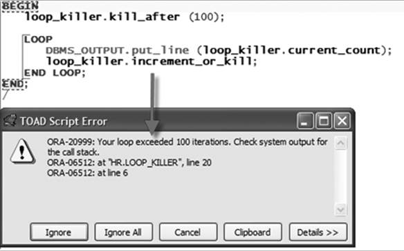
Figure 21-1. Using the Loop Killer package

Performance-Related Warnings

Oracle introduced a compile-time warnings framework in Oracle Database 10g PL/SQL. When you turn on warnings in your session, Oracle will give you feedback on the quality of your code, and will offer advice for improving readability and performance. I recommend that you use compile-time warnings to help identify areas of your code that could be optimized.

You can enable warnings for the entire set of performance-related warnings with the following statement:

ALTER SESSION SET PLSQL_WARNINGS = 'ENABLE:PERFORMANCE'

Performance warnings include the following:

§ PLW-06014: PLSQL_OPTIMIZE_LEVEL <= 1 turns off native code generation

§ PLW-07203: parameter “string” may benefit from use of the NOCOPY compiler hint

§ PLW-07204: conversion away from column type may result in suboptimal query plan

See Compile-Time Warnings for additional warnings and more details about working with these warnings. All of the warnings are documented in the Error Messages book of the Oracle documentation set.

The Optimizing Compiler

PL/SQL’s optimizing compiler can improve runtime performance dramatically, with a relatively slight cost at compile time. The benefits of optimization apply to both interpreted and natively compiled PL/SQL because the optimizing compiler applies optimizations by analyzing patterns in source code.

The optimizing compiler is enabled by default. However, you may want to alter its behavior, either by lowering its aggressiveness or by disabling it entirely. For example, if, in the course of normal operations, your system must perform recompilation of many lines of code, or if an application generates many lines of dynamically executed PL/SQL, the overhead of optimization may be unacceptable. Keep in mind, though, that Oracle’s tests show that the optimizer doubles the runtime performance of computationally intensive PL/SQL.

In some cases, the optimizer may even alter program behavior. One such case might occur in code written for Oracle9i Database that depends on the relative timing of initialization sections in multiple packages. If your testing demonstrates such a problem, yet you wish to enjoy the performance benefits of the optimizer, you may want to rewrite the offending code or to introduce an initialization routine that ensures the desired order of execution.

The optimizer settings are defined through the PLSQL_OPTIMIZE_LEVEL initialization parameter (and related ALTER DDL statements), which can be set to 0, 1, 2, or 3 (3 is available only in Oracle Database 11g and later). The higher the number, the more aggressive the optimization, meaning that the compiler will make a greater effort, and possibly restructure more of your code to optimize performance.

Set your optimization level according to the best fit for your application or program, as follows:

PLSQL_OPTIMIZE_LEVEL = 0

Zero essentially turns off optimization. The PL/SQL compiler maintains the original evaluation order of statement processing of Oracle9i Database and earlier releases. Your code will still run faster than in earlier versions, but the difference will not be so dramatic.

PLSQL_OPTIMIZE_LEVEL = 1

The compiler will apply many optimizations to your code, such as eliminating unnecessary computations and exceptions. It will not, in general, change the order of your original source code.

PLSQL_OPTIMIZE_LEVEL = 2

This is the default value. It is also the most aggressive setting available prior to Oracle Database 11g. It will apply many modern optimization techniques beyond those applied in level 1, and some of those changes may result in moving source code relatively far from its original location. Level 2 optimization offers the greatest boost in performance. It may, however, cause the compilation time in some of your programs to increase substantially. If you encounter this situation (or, alternatively, if you are developing your code and want to minimize compile time, knowing that when you move to production you will apply a higher optimization level), try cutting back the optimization level to 1.

PLSQL_OPTIMIZE_LEVEL = 3

Introduced in Oracle Database 11g, this level of optimization adds inlining of nested or local subprograms. It may be of benefit in extreme cases (large numbers of local subprograms or recursive execution), but for most PL/SQL applications, the default level of 2 should suffice.

You can set the optimization level for the instance as a whole, but then override the default for a session or for a particular program. For example:

ALTER SESSION SET PLSQL_OPTIMIZE_LEVEL = 0;

Oracle retains optimizer settings on a module-by-module basis. When you recompile a particular module with nondefault settings, the settings will “stick,” allowing you to recompile later using REUSE SETTINGS. For example:

ALTER PROCEDURE bigproc COMPILE PLSQL_OPTIMIZE_LEVEL = 0;

and then:

ALTER PROCEDURE bigproc COMPILE REUSE SETTINGS;

To view all the compiler settings for your modules, including optimizer level, interpreted versus native, and compiler warning levels, query the USER_PLSQL_OBJECT_SETTINGS view.

Insights on How the Optimizer Works

In addition to doing things that mere programmers are not allowed to do, optimizers can also detect and exploit patterns in your code that you might not notice. One of the chief methods that optimizers employ is reordering the work that needs to be done, to improve runtime efficiency. The definition of the programming language circumscribes the amount of reordering an optimizer can do, but PL/SQL’s definition leaves plenty of wiggle room—or “freedom”—for the optimizer. The rest of this section discusses some of the freedoms offered by PL/SQL, and gives examples of how code can be improved in light of them.

As a first example, consider the case of a loop invariant, something that is inside a loop but that remains constant over every iteration. Any programmer worth his salt will take a look at this:

FOR e IN (SELECT * FROM employees WHERE DEPT = p_dept)

LOOP

DBMS_OUTPUT.PUT_LINE('<DEPT>' || p_dept || '</DEPT>');

DBMS_OUTPUT.PUT_LINE('<emp ID="' || e.empno || '">');

etc.

END LOOP;

and tell you it would likely run faster if you pulled the “invariant” piece out of the loop, so it doesn’t reexecute needlessly:

l_dept_str := '<DEPT>' || p_dept || '</DEPT>'

FOR e IN (SELECT * FROM employees WHERE DEPT = p_dept)

LOOP

DBMS_OUTPUT.PUT_LINE(l_dept_str);

DBMS_OUTPUT.PUT_LINE('<emp ID="' || e.empno || '">');

etc.

END LOOP;

Even a salt-worthy programmer might decide, however, that the clarity of the first version outweighs the performance gains that the second would give you. Starting with Oracle Database 10g, PL/SQL no longer forces you to make this decision. With the default optimizer settings, the compiler will detect the pattern in the first version and convert it to bytecode that implements the second version. The reason this can happen is that the language definition does not require that loop invariants be executed repeatedly; this is one of the freedoms the optimizer can, and does, exploit. You might think that this optimization is a little thing, and it is, but the little things can add up. I’ve never seen a database that got smaller over time. Plenty of PL/SQL programs loop over all of the records in a growing table, and a million-row table is no longer considered unusually large. Personally, I’d be quite happy if Oracle would automatically eliminate a million unnecessary instructions from my code.

As another example, consider a series of statements such as these:

result1 := r * s * t;

...

result2 := r * s * v;

If there is no possibility of modifying r and s between these two statements, PL/SQL is free to compile the code like this:

interim := r * s;

result1 := interim * t;

...

result2 := interim * v;

The optimizer will take such a step if it thinks that storing the value in a temporary variable will be faster than repeating the multiplication.

Oracle has revealed these and other insights into the PL/SQL optimizer in a whitepaper, “Freedom, Order, and PL/SQL Compilation,” which is available on the Oracle Technology Network (enter the paper title in the search box). To summarize some of the paper’s main points:

§ Unless your code requires execution of a code fragment in a particular order by the rules of short-circuit expressions or of statement ordering, PL/SQL may execute the fragment in some order other than the one in which it was originally written. Reordering has a number of possible manifestations. In particular, the optimizer may change the order in which package initialization sections execute, and if a calling program only needs access to a package constant, the compiler may simply store that constant with the caller.

§ PL/SQL treats the evaluation of array indexes and the identification of fields in records as operators. If you have a nested collection of records and refer to a particular element and field such as price(product)(type).settle, PL/SQL must figure out an internal address that is associated with the variable. This address is treated as an expression; it may be stored and reused later in the program to avoid the cost of recomputation.

§ As shown earlier, PL/SQL may introduce interim values to avoid computations.

§ PL/SQL may completely eliminate operations such as x*0. However, an explicit function call will not be eliminated; in the expression f()*0, the function f() will always be called in case there are side effects.

§ PL/SQL does not introduce new exceptions.

§ PL/SQL may obviate the raising of exceptions. For example, the divide by 0 exception in this code can be dropped because it is unreachable:

IF FALSE THEN y := x/0; END IF;

PL/SQL does not have the freedom to change which exception handler will handle a given exception.

Point 1 deserves a bit of elaboration. In the applications that I write, I’m accustomed to taking advantage of package initialization sections, but I’ve never really worried about execution order. My initialization sections are typically small and involve the assignment of static lookup values (typically retrieved from the database), and these operations seem to be immune from the order of operations. If your application must guarantee the order of execution, you’ll want to move the code out of the initialization section and put it into separate initialization routines you invoke explicitly. For example, you would call:

pkgA.init();

pkgB.init();

right where you need pkgA and then pkgB initialized. This advice holds true even if you are not using the optimizing compiler.

Point 2 also deserves some comment. The example is price(product)(type).settle. If this element is referenced several times where the value of the variable type is changing but the value of the variable product is not, then optimization might split the addressing into two parts—the first to compute price(product) and the second (used in several places) to compute the rest of the address. The code will run faster because only the changeable part of the address is recomputed each time the entire reference is used. More importantly, this is one of those changes that the compiler can make easily, but that would be very difficult for the programmer to make in the original source code because of the semantics of PL/SQL. Many of the optimization changes are of this ilk; the compiler can operate “under the hood” to do something the programmer would find difficult.

PL/SQL includes other features to identify and speed up certain programming idioms. In this code:

counter := counter + 1;

the compiler does not generate machine code that does the complete addition. Instead, PL/SQL detects this programming idiom and uses a special PL/SQL virtual machine (PVM) “increment” instruction that runs much faster than the conventional addition (this applies to a subset of numeric datatypes—PLS_INTEGER and SIMPLE_INTEGER—but will not happen with NUMBER).

A special instruction also exists to handle code that concatenates many terms:

str := 'value1' || 'value2' || 'value3' ...

Rather than treating this as a series of pairwise concatenations, the compiler and PVM work together and do the series of concatenations in a single instruction.

Most of the rewriting that the optimizer does will be invisible to you. During an upgrade, you may find a program that is not as well behaved as you thought, because it relied on an order of execution that the new compiler has changed. It seems likely that a common problem area will be the order of package initialization, but of course your mileage may vary.

One final comment: the way the optimizer modifies code is deterministic, at least for a given value of PLSQL_OPTIMIZE_LEVEL. In other words, if you write, compile, and test your program using, say, the default optimizer level of 2, its behavior will not change when you move the program to a different computer or a different database—as long as the destination database version and optimizer level are the same.

Runtime Optimization of Fetch Loops

For database versions up through and including Oracle9i Database Release 2, a cursor FOR loop such as the following would retrieve exactly one logical row per fetch.

FOR arow IN (SELECT something FROM somewhere)

LOOP

...

END LOOP;

So, if you had 500 rows to retrieve, there would be 500 fetches, and therefore 500 expensive “context switches” between PL/SQL and SQL.

However, starting with Oracle Database 10g, the database performs an automatic “bulkification” of this construct so that each fetch retrieves (up to) 100 rows. The preceding cursor FOR loop would use only five fetches to bring the 500 rows back from the SQL engine. It’s as if the database automatically recodes your loop to use the BULK COLLECT feature (described later in this chapter).

This apparently undocumented feature also works for code of the form:

FOR arow IN cursorname

LOOP

...

END LOOP;

However, it does not work with code of the form:

OPEN cursorname;

LOOP

EXIT WHEN cursorname%NOTFOUND;

FETCH cursorname INTO ...

END LOOP;

CLOSE cursorname;

Nevertheless, this internal optimization should be a big win for the cursor FOR loop case (which has the added benefit of conciseness).

Data Caching Techniques

A very common technique for improving performance is to build caches for data that needs to be accessed repeatedly—and that is, at least for some period of time, static (does not change).

The SGA of the Oracle database is the “mother of all caches,” Oracle-wise. It is a (usually) very large and (always) very complex area of memory that serves as the intermediary between the actual database (files on disk) and the programs that manipulate that database.

As described more thoroughly in Chapter 20, the SGA caches the following information (and much more, but these are the most relevant for PL/SQL programmers):

§ Parsed cursors

§ Data queried by cursors from the database

§ Partially compiled representations of our programs

For the most part, however, the database does not use the SGA to cache program data. When you declare a variable in your program, the memory for that data is consumed in the PGA (for dedicated server). Each connection to the database has its own PGA; the memory required to store your program data is, therefore, copied in each connection that calls that program.

Fortunately, there is a benefit to the use of PGA memory: your PL/SQL program can retrieve information more quickly from the PGA than it can from the SGA. Thus, PGA-based caching offers some interesting opportunities to improve performance. Oracle also provides other PL/SQL-specific caching mechanisms to help improve the performance of your programs. In this section, you will learn about three types of PL/SQL caching (another technique you might consider utilizes application contexts):

Package-based caching

Use the UGA memory area to store static data that you need to retrieve many times. Use PL/SQL programs to avoid repeatedly accessing data via the SQL layer in the SGA. This is the fastest caching technique, but also the most restrictive in terms of circumstances when it can safely be used.

Deterministic function caching

When you declare a function to be deterministic and call that function inside a SQL statement, Oracle will cache the inputs to the function and its return value. If you call the function with the same inputs, Oracle may return the previously stored value without calling the function.

Function result caching (Oracle Database 11g and later)

This latest advance in PL/SQL caching is the most exciting and useful. With a simple declarative clause in your function header, you can instruct the database to cache the function’s input and return values. In contrast to the deterministic approach, however, the function result cache is used whenever the function is called (not just from within a SQL statement), and the cache is automatically invalidated when dependent data changes.

NOTE

When you use a package-based cache, you store a copy of the data. You need to be very certain that your copy is accurate and up to date. It is quite possible to abuse each of these caching approaches and end up with “dirty data” being served up to users.

Package-Based Caching

A package-based cache consists of one or more variables declared at the package level, rather than in any subprogram of the package. Package-level data is a candidate for caching, because this kind of data persists throughout a session, even if programs in that session are not currently using the data or calling any of the subprograms in the package. In other words, if you declare a variable at the package level, once you assign a value to that variable it keeps that value until you disconnect, recompile the package, or change the value.

I will explore package-based caching by first describing the scenarios under which you will want to use this technique. Then I will look at a simple example of caching a single value. Finally, I will show you how you can cache all or part of a relational table in a package, and thereby greatly speed up access to the data in that table.

When to use package-based caching

Consider using a package-based cache under the following circumstances:

§ You are not yet using Oracle Database 11g or higher. If you are developing applications for recent releases, you will almost always be better off using the function result cache, not a package-based cache.

§ The data you wish to cache does not change for the duration of time that the data is needed by a user. Examples of static data include small reference tables (“O” is for “Open,” “C” is for “Closed,” etc.) that rarely, if ever, change, and batch scripts that require a “snapshot” of consistent data taken at the time the script starts and used until the script ends.

§ Your database server has enough memory to support a copy of your cache for each session connected to the instance (and using your cache). You can use the utility described earlier in this chapter to measure the size of the cache defined in your package.

Conversely, do not use a package-based cache if either of the following is true:

§ The data you are caching could possibly change during the time the user is accessing the cache.

§ The volume of data cached requires too much memory per session, causing memory errors with large numbers of users.

A simple example of package-based caching

Consider the USER function—it returns the name of the currently connected session. Oracle implements this function in the STANDARD package as follows:

function USER return varchar2 is

c varchar2(255);

begin

select user into c from sys.dual;

return c;

end;

Thus, every time you call USER, you execute a query. Sure, it’s a fast query, but it should never be executed more than once in a session, since the value never changes. You are probably now saying to yourself: so what? Not only is a SELECT FROM dual very efficient, but the Oracle database will also cache the parsed query and the value returned, so it is already very optimized. Would package-based caching make any difference? Absolutely!

Consider the following package:

/* File on web: thisuser.pkg */

PACKAGE thisuser

IS

cname CONSTANT VARCHAR2(30) := USER;

FUNCTION name RETURN VARCHAR2;

END;

PACKAGE BODY thisuser

IS

g_user VARCHAR2(30) := USER;

FUNCTION name RETURN VARCHAR2 IS BEGIN RETURN g_user; END;

END;

I cache the value returned by USER in two different ways:

§ A constant defined at the package level. The PL/SQL runtime engine calls USER to initialize the constant when the package is initialized (on first use).

§ A function. The function returns the name of “this user”—the value returned by the function is a private (package body) variable also assigned the value returned by USER when the package is initialized.

Having now created these caches, I should see if they are worth the bother. Is either implementation noticeably faster than simply calling the highly optimized USER function over and over?

So, I build a script utilizing sf_timer to compare performance:

/* File on web: thisuser.tst */

PROCEDURE test_thisuser (count_in IN PLS_INTEGER)

IS

l_name all_users.username%TYPE;

BEGIN

sf_timer.start_timer;

FOR indx IN 1 .. count_in LOOP l_name := thisuser.NAME; END LOOP;

sf_timer.show_elapsed_time ('Packaged Function');

--

sf_timer.start_timer;

FOR indx IN 1 .. count_in LOOP l_name := thisuser.cname; END LOOP;

sf_timer.show_elapsed_time ('Packaged Constant');

--

sf_timer.start_timer;

FOR indx IN 1 .. count_in LOOP l_name := USER; END LOOP;

sf_timer.show_elapsed_time ('USER Function');

END test_thisuser;

And when I run it for 100 and then 1,000,000 iterations, I see these results:

Packaged Function Elapsed: 0 seconds.

Packaged Constant Elapsed: 0 seconds.

USER Function Elapsed: 0 seconds.

Packaged Function Elapsed: .48 seconds.

Packaged Constant Elapsed: .06 seconds.

USER Function Elapsed: 32.6 seconds.

The results are clear: for small numbers of iterations, the advantage of caching is not apparent. However, for large numbers of iterations, the package-based cache is dramatically faster than going through the SQL layer and the SGA.

Also, accessing the constant is faster than calling a function that returns the value. So why use a function? The function version offers this advantage over the constant: it hides the value. So, if for any reason the value must be changed (not applicable to this scenario), you can do so without recompiling the package specification, which would force recompilation of all programs dependent on this package.

While it is unlikely that you will ever benefit from caching the value returned by the USER function, I hope you can see that package-based caching is clearly a very efficient way to store and retrieve data. Now let’s take a look at a less trivial example.

Caching table contents in a package

If your application includes a table that never changes during normal working hours (that is, it is static while a user accesses the table), you can rather easily create a package that caches the full contents of that table, boosting query performance by an order of magnitude or more.

Suppose that I have a table of products that is static, defined as follows:

/* File on web: package_cache_demo.sql */

TABLE products (

product_number INTEGER PRIMARY KEY

, description VARCHAR2(1000))

Here is a package body that offers two ways of querying data from this table—query each time or cache the data and retrieve it from the cache:

1 PACKAGE BODY products_cache

2 IS

3 TYPE cache_t IS TABLE OF products%ROWTYPE INDEX BY PLS_INTEGER;

4 g_cache cache_t;

5

6 FUNCTION with_sql (product_number_in IN products.product_number%TYPE)

7 RETURN products%ROWTYPE

8 IS

9 l_row products%ROWTYPE;

10 BEGIN

11 SELECT * INTO l_row FROM products

12 WHERE product_number = product_number_in;

13 RETURN l_row;

14 END with_sql;

15

16 FUNCTION from_cache (product_number_in IN products.product_number%TYPE)

17 RETURN products%ROWTYPE

18 IS

19 BEGIN

20 RETURN g_cache (product_number_in);

21 END from_cache;

22 BEGIN

23 FOR product_rec IN (SELECT * FROM products) LOOP

24 g_cache (product_rec.product_number) := product_rec;

25 END LOOP;

26 END products_cache;

The following table explains the interesting parts of this package.

With this code in place, the first time a user calls the from_cache (or with_sql) function, the database will first execute this code.

Next, I construct and run a block of code to compare the performance of these approaches:

DECLARE

l_row products%ROWTYPE;

BEGIN

sf_timer.start_timer;

FOR indx IN 1 .. 100000

LOOP

l_row := products_cache.from_cache (5000);

END LOOP;

sf_timer.show_elapsed_time ('Cache table');

--

sf_timer.start_timer;

FOR indx IN 1 .. 100000

LOOP

l_row := products_cache.with_sql (5000);

END LOOP;

sf_timer.show_elapsed_time ('Run query every time');

END;

And here are the results I see:

Cache table Elapsed: .14 seconds.

Run query every time Elapsed: 4.7 seconds.

Again, it is very clear that package-based caching is much, much faster than executing a query repeatedly—even when that query is fully optimized by all the power and sophistication of the SGA.

Just-in-time caching of table data

Suppose I have identified a static table to which I want to apply this caching technique. There is, however, a problem: the table has 100,000 rows of data. I can build a package like products_cache, shown in the previous section, but it uses 5 MB of memory in each session’s PGA. With 500 simultaneous connections, this cache will consume 2.5 GB, which is unacceptable. Fortunately, I notice that even though the table has many rows of data, each user will typically query only the same 50 or so rows of that data (there are, in other words, hot spots of activity). So, caching the full table in each session is wasteful in terms of both CPU cycles (the initial load of 100,000 rows) and memory.

When your table is static, but you don’t want or need all the data in that table, you should consider employing a “just in time” approach to caching. This means that you do not query the full contents of the table into your collection cache when the package initializes. Instead, whenever the user asks for a row, if it is in the cache, you return it immediately. If not, you query that single row from the table, add it to the cache, and then return the data.

The next time the user asks for that same row, it will be retrieved from the cache. The following code demonstrates this approach:

/* File on web: package_cache_demo.sql */

FUNCTION jit_from_cache (product_number_in IN products.product_number%TYPE)

RETURN products%ROWTYPE

IS

l_row products%ROWTYPE;

BEGIN

IF g_cache.EXISTS (product_number_in)

THEN

/* Already in the cache, so return it. */

l_row := g_cache (product_number_in);

ELSE

/* First request, so query it from the database

and then add it to the cache. */

l_row := with_sql (product_number_in);

g_cache (product_number_in) := l_row;

END IF;

RETURN l_row;

END jit_from_cache;

Generally, just-in-time caching is somewhat slower than the one-time load of all data to the cache, but it is still much faster than repeated database lookups.

Deterministic Function Caching

A function is considered deterministic if it returns the same result value whenever it is called with the same values for its IN and IN OUT arguments. Another way to think about deterministic programs is that they have no side effects. Everything the program changes is reflected in the parameter list. See Chapter 17 for more details on deterministic functions.

Precisely because a deterministic function behaves so consistently, Oracle can build a cache from the function’s inputs and outputs. After all, if the same inputs always result in the same outputs, then there is no reason to call the function a second time if the inputs match a previous invocation of that function.

Let’s take a look at an example of the caching nature of deterministic functions. Suppose I define the following encapsulation on top of SUBSTR (return the string between the start and end locations) as a deterministic function:

/* File on web: deterministic_demo.sql */

FUNCTION betwnstr (

string_in IN VARCHAR2, start_in IN PLS_INTEGER, end_in IN PLS_INTEGER)

RETURN VARCHAR2 DETERMINISTIC

IS

BEGIN

RETURN (SUBSTR (string_in, start_in, end_in - start_in + 1));

END betwnstr;

I can then call this function inside a query (it does not modify any database tables, which would otherwise preclude using it in this way), such as:

SELECT betwnstr (last_name, 1, 5) first_five

FROM employees

And when betwnstr is called in this way, the database will build a cache of inputs and their return values. Then, if I call the function again with the same inputs, the database will return the value without calling the function. To demonstrate this optimization, I will change betwnstr to the following:

FUNCTION betwnstr (

string_in IN VARCHAR2, start_in IN PLS_INTEGER, end_in IN PLS_INTEGER)

RETURN VARCHAR2 DETERMINISTIC

IS

BEGIN

DBMS_LOCK.sleep (.01);

RETURN (SUBSTR (string_in, start_in, end_in - start_in + 1));

END betwnstr;

In other words, I will use the sleep subprogram of DBMS_LOCK to pause betwnstr for 1/100th of a second.

If I call this function in a PL/SQL block of code (not from within a query), the database will not cache the function values, so when I query the 107 rows of the employees table it will take more than one second:

DECLARE

l_string employees.last_name%TYPE;

BEGIN

sf_timer.start_timer;

FOR rec IN (SELECT * FROM employees)

LOOP

l_string := betwnstr ('FEUERSTEIN', 1, 5);

END LOOP;

sf_timer.show_elapsed_time ('Deterministic function in block');

END;

/

The output is:

Deterministic function in block Elapsed: 1.67 seconds.

If I now execute the same logic, but move the call to betwnstr inside the query, the performance is quite different:

BEGIN

sf_timer.start_timer;

FOR rec IN (SELECT betwnstr ('FEUERSTEIN', 1, 5) FROM employees)

LOOP

NULL;

END LOOP;

sf_timer.show_elapsed_time ('Deterministic function in query');

END;

/

The output is:

Deterministic function in query Elapsed: .05 seconds.

As you can see, caching with a deterministic function is a very effective path to optimization. Just be sure of the following:

§ When you declare a function to be deterministic, make sure that it really is. The Oracle database does not analyze your program to determine if you are telling the truth. If you add the DETERMINISTIC keyword to a function that, for example, queries data from a table, the database might cache data inappropriately, with the consequence that a user sees “dirty data.”

§ You must call that function within a SQL statement to get the effects of deterministic caching; that is a significant constraint on the usefulness of this type of caching.

THe Function Result Cache (Oracle Database 11g)

Prior to the release of Oracle Database 11g, package-based caching offered the best, most flexible option for caching data for use in a PL/SQL program. Sadly, the circumstances under which it can be used are quite limited, since the data source must be static and memory consumption grows with each session connected to the Oracle database.

Recognizing the performance benefit of this kind of caching (as well as that implemented for deterministic functions), Oracle implemented the function result cache in Oracle Database 11g. This feature offers a caching solution that overcomes the weaknesses of package-based caching and offers performance that is almost as fast.

When you turn on the function result cache for a function, you get the following benefits:

§ Oracle stores both inputs and their return values in a separate cache for each function. The cache is shared among all sessions connected to this instance of the database; it is not duplicated for each session. In Oracle Database 11g Release 2 and later, the function result cache is even shared across instances in a Real Application Cluster (RAC).

§ Whenever the function is called, the database checks to see if it has already cached the same input values. If so, then the function is not executed. The value stored in the cache is simply returned.

§ Whenever changes are committed to tables that are identified as dependencies for the cache, the database automatically invalidates the cache. Subsequent calls to the function will then repopulate the cache with consistent data.

§ Caching occurs whenever the function is called; you do not need to invoke it within a SQL statement.

§ There is no need to write code to declare and populate a collection; instead, you use declarative syntax in the function header to specify the cache.

You will most likely use the result cache feature with functions that query data from tables. Excellent candidates for result caching are:

§ Static datasets, such as materialized views. The contents of these views do not change between their refreshes, so why fetch the data multiple times?

§ Tables that are queried much more frequently than they are changed. If a table is changed on average every five minutes, but in between changes the same rows are queried hundreds or thousands of times, the result cache can be used to good effect.

If, however, your table is changed every second, you do not want to cache the results; it could actually slow down your application, as Oracle will spend lots of time populating and then clearing out the cache. Choose carefully how and where to apply this feature, and work closely with your DBA to ensure that the SGA pool for the result cache is large enough to hold all the data you expect to be cached during typical production usage.

In the following sections, I will first describe the syntax of this feature. Then I will demonstrate some simple examples of using the result cache, discuss the circumstances under which you should use it, cover the DBA-related aspects of cache management, and review restrictions and gotchas for this feature.

Enabling the function result cache

Oracle has made it very easy to add function result caching to your functions. You simply need to add the RESULT_CACHE clause to the header of your function, and Oracle takes it from there.

The syntax of the RESULT_CACHE clause is:

RESULT_CACHE [ RELIES_ON (table_or_view [, table_or_view2 ... table_or_viewN] ]

The RELIES_ON clause tells Oracle which tables or views the contents of the cache rely upon. This clause can only be added to the headers of schema-level functions and the implementation of a packaged function (that is, in the package body). As of Oracle Database 11g Release 2, it is deprecated. Here is an example of a packaged function—note that the RESULT_CACHE clause must appear in both specification and body:

CREATE OR REPLACE PACKAGE get_data

IS

FUNCTION session_constant RETURN VARCHAR2 RESULT_CACHE;

END get_data;

/

CREATE OR REPLACE PACKAGE BODY get_data

IS

FUNCTION session_constant RETURN VARCHAR2

RESULT_CACHE

IS

BEGIN

...

END session_constant;

END get_data;

/

Such an elegant feature; just add one clause to the header of your function, and see a significant improvement in performance!

The RELIES_ON clause (deprecated in 11.2)

The first thing to understand about RELIES_ON is that it is no longer needed as of Oracle Database 11g Release 2. Starting with that version, Oracle will automatically determine which tables your returned data is dependent upon and correctly invalidate the cache when those tables’ contents are changed; including your own RELIES_ON clause does nothing. Run the 11gR2_frc_no_relies_on.sql script available on the book’s website to verify this behavior. This analysis identifies tables that are referenced through static (embedded) or dynamic SQL, as well as tables that are referenced only indirectly (through views).

If you are running Oracle Database 11g Release 1 or earlier, however, it is up to you to explicitly list all tables and views from which returned data is queried. Determining which tables and views to include in the list is usually fairly straightforward. If your function contains a SELECT statement, then make sure that any tables or views in any FROM clause in that query are added to the list.

If you select from a view, you need to list only that view, not all the tables that are queried from within the view. The script named 11g_frc_views.sql, also available on the website, demonstrates how the database will determine from the view definition itself all the tables whose changes must invalidate the cache.

Here are some examples of using the RELIES_ON clause:

1. As schema-level function with a RELIES_ON clause indicating that the cache relies on the employees table:

2. CREATE OR REPLACE FUNCTION name_for_id (id_in IN employees.employee_id%TYPE)

3. RETURN employees.last_name%TYPE

RESULT_CACHE RELIES ON (employees)

4. A packaged function with a RELIES_ON clause (it may appear only in the body):

5. CREATE OR REPLACE PACKAGE get_data

6. IS

7. FUNCTION name_for_id (id_in IN employees.employee_id%TYPE)

8. RETURN employees.last_name%TYPE

9. RESULT_CACHE

10.END get_data;

11./

12.

13.CREATE OR REPLACE PACKAGE BODY get_data

14.IS

15. FUNCTION name_for_id (id_in IN employees.employee_id%TYPE)

16. RETURN employees.last_name%TYPE

17. RESULT_CACHE RELIES ON (employees)

18. IS

19. BEGIN

20. ...

21. END name_for_id;

22.END get_data;

/

23.A RELIES_ON clause with multiple objects listed:

24.CREATE OR REPLACE PACKAGE BODY get_data

25.IS

26. FUNCTION name_for_id (id_in IN employees.employee_id%TYPE)

27. RETURN employees.last_name%TYPE

28. RESULT_CACHE RELIES ON (employees, departments, locations)

...

Function result cache example: A deterministic function

In a previous section I talked about the caching associated with deterministic functions. In particular, I noted that this caching will only come into play when the function is called within a query. Let’s now apply the Oracle Database 11g function result cache to the betwnstr function and see that it works when called natively in a PL/SQL block.

In the following function, I add the RESULT_CACHE clause to the header. I also add a call to DBMS_OUTPUT.PUT_LINE to show what inputs were passed to the function:

/* File on web: 11g_frc_simple_demo.sql */

FUNCTION betwnstr (

string_in IN VARCHAR2, start_in IN INTEGER, end_in IN INTEGER)

RETURN VARCHAR2 RESULT_CACHE

IS

BEGIN

DBMS_OUTPUT.put_line (

'betwnstr for ' || string_in || '-' || start_in || '-' || end_in);

RETURN (SUBSTR (string_in, start_in, end_in - start_in + 1));

END;

I then call this function for 10 rows in the employees table. If the employee ID is even, then I apply betwnstr to the employee’s last name. Otherwise, I pass it the same three input values:

DECLARE

l_string employees.last_name%TYPE;

BEGIN

FOR rec IN (SELECT * FROM employees WHERE ROWNUM < 11)

LOOP

l_string :=

CASE MOD (rec.employee_id, 2)

WHEN 0 THEN betwnstr (rec.last_name, 1, 5)

ELSE betwnstr ('FEUERSTEIN', 1, 5)

END;

END LOOP;

END;

When I run this function, I see the following output:

betwnstr for OConnell-1-5

betwnstr for FEUERSTEIN-1-5

betwnstr for Whalen-1-5

betwnstr for Fay-1-5

betwnstr for Baer-1-5

betwnstr for Gietz-1-5

betwnstr for King-1-5

Notice that FEUERSTEIN appears only once, even though it was called five times. That demonstrates the function result cache in action.

Function result cache example: Querying data from a table

You will mostly want to use the function result cache when you are querying data from a table whose contents are queried more frequently than they are changed (in between changes, the data is static). Suppose, for example, that in my real estate management application I have a table that contains the interest rates available for different types of loans. The contents of this table are updated via a scheduled job that runs once an hour throughout the day. Here is the structure of the table and the data I am using in my demonstration script:

/* File on web: 11g_frc_demo_table.sql */

CREATE TABLE loan_info (

NAME VARCHAR2(100) PRIMARY KEY,

length_of_loan INTEGER,

initial_interest_rate NUMBER,

regular_interest_rate NUMBER,

percentage_down_payment INTEGER)

/

BEGIN

INSERT INTO loan_info VALUES ('Five year fixed', 5, 6, 6, 20);

INSERT INTO loan_info VALUES ('Ten year fixed', 10, 5.7, 5.7, 20);

INSERT INTO loan_info VALUES ('Fifteen year fixed', 15, 5.5, 5.5, 10);

INSERT INTO loan_info VALUES ('Thirty year fixed', 30, 5, 5, 10);

INSERT INTO loan_info VALUES ('Two year balloon', 2, 3, 8, 0);

INSERT INTO loan_info VALUES ('Five year balloon', 5, 4, 10, 5);

COMMIT;

END;

/

Here is a function to retrieve all the information for a single row:

FUNCTION loan_info_for_name (NAME_IN IN VARCHAR2)

RETURN loan_info%ROWTYPE

RESULT_CACHE RELIES_ON (loan_info)

IS

l_row loan_info%ROWTYPE;

BEGIN

DBMS_OUTPUT.put_line ('> Looking up loan info for ' || NAME_IN);

SELECT * INTO l_row FROM loan_info WHERE NAME = NAME_IN;

RETURN l_row;

END loan_info_for_name;

In this case, the RESULT_CACHE clause includes the RELIES_ON subclause to indicate that the cache for this function is based on data from (“relies on”) the loan_info table. I then run the following script, which calls the function for two different names, then changes the contents of the table, and finally calls the function again for one of the original names:

DECLARE

l_row loan_info%ROWTYPE;

BEGIN

DBMS_OUTPUT.put_line ('First time for Five year fixed...');

l_row := loan_info_for_name ('Five year fixed');

DBMS_OUTPUT.put_line ('First time for Five year balloon...');

l_row := loan_info_for_name ('Five year balloon');

DBMS_OUTPUT.put_line ('Second time for Five year fixed...');

l_row := loan_info_for_name ('Five year fixed');

UPDATE loan_info SET percentage_down_payment = 25

WHERE NAME = 'Thirty year fixed';

COMMIT;

DBMS_OUTPUT.put_line ('After commit, third time for Five year fixed...');

l_row := loan_info_for_name ('Five year fixed');

END;

Here’s the output from running this script:

First time for Five year fixed...

> Looking up loan info for Five year fixed

First time for Five year balloon...

> Looking up loan info for Five year balloon

Second time for Five year fixed...

After commit, third time for Five year fixed...

> Looking up loan info for Five year fixed

And here is an explanation of what you see happening here:

§ The first time I call the function for “Five year fixed” the PL/SQL runtime engine executes the function, looks up the data, puts the data in the cache, and returns the data.

§ The first time I call the function for “Five year balloon” it executes the function, looks up the data, puts the data in the cache, and returns the data.

§ The second time I call the function for “Five year fixed”, it does not execute the function (there is no “Looking up...” for the second call). The function result cache at work...

§ Then I change a column value for the row with name “Thirty year fixed” and commit that change.

§ Finally, I call the function for the third time for “Five year fixed”. This time, the function is again executed to query the data. This happens because I have told Oracle that this RESULT_CACHE RELIES_ON the loan_info table, and the contents of that table have changed.

Function result cache example: Caching a collection

So far I have shown you examples of caching an individual value and an entire record. You can also cache an entire collection of data, even a collection of records. In the following code, I have changed the function to return all of the names of loans into a collection of strings (based on the predefined DBMS_SQL collection type). I then call the function repeatedly, but the collection is populated only once (BULK COLLECT is described later in this chapter):

/* File on web: 11g_frc_table_demo.sql */

FUNCTION loan_names RETURN DBMS_SQL.VARCHAR2S

RESULT_CACHE RELIES_ON (loan_info)

IS

l_names DBMS_SQL.VARCHAR2S;

BEGIN

DBMS_OUTPUT.put_line ('> Looking up loan names....');

SELECT name BULK COLLECT INTO l_names FROM loan_info;

RETURN l_names;

END loan_names;

Here is a script that demonstrates that even when populating a complex type like this, the function result cache will come into play:

DECLARE

l_names DBMS_SQL.VARCHAR2S;

BEGIN

DBMS_OUTPUT.put_line ('First time retrieving all names...');

l_names := loan_names ();

DBMS_OUTPUT.put_line('Second time retrieving all names...');

l_names := loan_names ();

UPDATE loan_info SET percentage_down_payment = 25

WHERE NAME = 'Thirty year fixed';

COMMIT;

DBMS_OUTPUT.put_line ('After commit, third time retrieving all names...');

l_names := loan_names ();

END;

/

The output is:

First time retrieving all names...

> Looking up loan names....

Second time retrieving all names...

After commit, third time retrieving all names...

> Looking up loan names....

When to use the function result cache

Caching must always be done with the greatest of care. If you cache incorrectly, your application may deliver bad data to users. The function result cache is the most flexible and widely useful of the different types of caches you can use in PL/SQL code, but you can still get yourself in trouble with it.

You should consider adding RESULT_CACHE to your function header in any of the following circumstances:

§ Data is queried from a table more frequently than it is updated. Suppose, for example, that in my Human Resources application, users query the contents of the employees table thousands of times a minute, but it is updated on average once every 10 minutes. In between those changes, the employees table is static, so the data can safely be cached—and the query time reduced.

§ A function that doesn’t query any data is called repeatedly (often, in this scenario, recursively) with the same input values. One classic example from programming texts is the Fibonacci algorithm. To calculate the Fibonacci value for the integer n—that is, F(n)—you must compute F(1) through F(n−1) multiple times.

§ Your application (or each user of the application) relies on a set of configuration values that are static during use of the application: a perfect fit for the function result cache!

When not to use the function result cache

You cannot use the RESULT_CACHE clause if any of the following are true:

§ The function is defined within the declaration section of an anonymous block. To be result-cached, the function must be defined at the schema level or within a package.

§ The function is a pipelined table function.

§ The function has any OUT or IN OUT parameters. In this case, the function can only return data through the RETURN clause.

§ Any of the function’s IN parameters are of any of these types: BLOB, CLOB, NCLOB, REF CURSOR, collection, record, or object type.

§ The function RETURN type is any of the following: BLOB, CLOB, NCLOB, REF CURSOR, object type, or a collection or record that contains any of the previously listed datatypes (for example, a collection of CLOBs would be a no-go for function result caching).

§ The function is an invoker rights function and you are using Oracle Database 11g. In 11g, an attempt to define a function as both result-cached and using invoker rights resulted in this compilation error: PLS-00999: implementation restriction (may be temporary) RESULT_CACHE is disallowed on subprograms in Invoker-Rights modules. Good news: this implementation restriction was lifted in Oracle Database 12c, allowing caching of results from functions defined with the AUTHID CURRENT_USER clause. Conceptually, it is as if Oracle is passing the username as an invisible argument to the function.

§ The function references data dictionary tables, temporary tables, sequences, or nondeterministic SQL functions.

You should not use (or at a minimum very carefully evaluate your use of) the RESULT_CACHE clause if any of the following is true:

§ Your function has side effects; for example, it modifies the contents of database tables or modifies the external state of your application (by, for example, sending data to sysout via DBMS_OUTPUT or sending email). Since you can never be sure when and if the body of the function will execute, your application will likely not perform correctly under all circumstances. This is an unacceptable tradeoff for improved performance.

§ Your function (or the query inside it) contains session-specific dependencies, such as a reference to SYSDATE or USER, dependencies on NLS settings (such as with a call to TO_CHAR that relies on the default format model), and so on.

§ Your function executes a query against a table on which a Virtual Private Database (VPD) security policy applies. I explore the ramifications of using VPD with function result caching, in the section Fine-grained dependencies in 11.2 and higher.

Useful details of function result cache behavior

The following information should come in handy as you delve into the details of applying the function result cache to your application:

§ When checking to see if the function has been called previously with the same inputs, Oracle considers NULL to be equal to NULL. In other words, if my function has one string argument and it is called with a NULL input value, then the next time it is called with a NULL value, Oracle will decide that it does not need to call the function and can instead return the cached outcome.

§ Users never see dirty data. Suppose a result cache function returns the last name of an employee for an ID, and that the last name “Feuerstein” is cached for ID 400. If a user then changes the contents of the employees table, even if that change has not yet been committed, the database will bypass the cache (and any other cache that relies on employees) for that user’s session. All other users connected to the instance (or RAC, in Oracle Database 11g Release 2 and later) will continue to take advantage of the cache.

§ If the function propagates an unhandled exception, the database will not cache the input values for that execution; that is, the contents of the result cache for this function will not be changed.

Managing the function result cache

The function result cache is an area of memory in the SGA. Oracle provides the usual cast of characters so that a database administrator can manage that cache:

RESULT_CACHE_MAX_SIZE initialization parameter

Specifies the maximum amount of SGA memory that the function result cache can use. When the cache fills up, Oracle will use the least recently used algorithm to age out of the cache the data that has been there the longest.

DBMS_RESULT_CACHE package

Supplied package that offers a set of subprograms to manage the contents of the cache. This package will mostly be of interest to database administrators.

Dynamic performance views

V$RESULT_CACHE_STATISTICS

Displays various result cache settings and usage statistics, including block size and the number of cache results successfully created

V$RESULT_CACHE_OBJECTS

Displays all the objects for which results have been cached

V$RESULT_CACHE_MEMORY

Displays all the memory blocks and their status, linking back to the V%RESULT_CACHE_OBJECTS view through the object_id column

V$RESULT_CACHE_DEPENDENCY

Displays the depends-on relationship between cached results and dependencies

Here is a procedure you can use to display dependencies:

/* File on web: show_frc_dependencies.sql */

CREATE OR REPLACE PROCEDURE show_frc_dependencies (

name_like_in IN VARCHAR2)

IS

BEGIN

DBMS_OUTPUT.put_line ('Dependencies for "' || name_like_in || '"');

FOR rec

IN (SELECT d.result_id

/* Clean up display of function name */

, TRANSLATE (SUBSTR (res.name, 1, INSTR (res.name, ':') - 1)

, 'A"', 'A')

function_name

, dep.name depends_on

FROM v$result_cache_dependency d

, v$result_cache_objects res

, v$result_cache_objects dep

WHERE res.id = d.result_id

AND dep.id = d.depend_id

AND res.name LIKE name_like_in)

LOOP

/* Do not include dependency on self */

IF rec.function_name <> rec.depends_on

THEN

DBMS_OUTPUT.put_line (

rec.function_name || ' depends on ' || rec.depends_on);

END IF;

END LOOP;

END;

/

Fine-grained dependencies in 11.2 and higher

A significant enhancement in 11.2 for the function result cache feature is fine-grained dependency tracking. Oracle now remembers specifically which tables each set of cached data (IN argument values and the result) depends on. In other words, different rows of cached data may have different sets of dependent tables. And when changes to a table are committed, Oracle will remove or flush only those results from the cache that are dependent on that table, not necessarily the entire cache (as would have happened in 11.1).

Most of the functions to which you apply the result cache feature will have the same table dependencies, regardless of the actual values passed for the formal parameters. The following is an example in which table dependencies can change:

/* File on web: 11g_frc_dependencies.sql */

CREATE TABLE tablea (col VARCHAR2 (2));

CREATE TABLE tableb (col VARCHAR2 (2));

BEGIN

INSERT INTO tablea VALUES ('a1');

INSERT INTO tableb VALUES ('b1');

COMMIT;

END;

/

CREATE OR REPLACE FUNCTION dynamic_query (table_suffix_in VARCHAR2)

RETURN VARCHAR2

RESULT_CACHE

IS

l_return VARCHAR2 (2);

BEGIN

DBMS_OUTPUT.put_line ('SELECT FROM table' || table_suffix_in);

EXECUTE IMMEDIATE 'select col from table' || table_suffix_in INTO l_return;

RETURN l_return;

END;

/

As you can see, if I pass a for the table suffix parameter, then the function will fetch a row from TABLEA. But if I pass b, then the function will fetch a row from TABLEB. Now suppose I execute the following script, which uses the procedure defined in the previous section to show the changes in the result cache, and its dependencies:

/* File on web: 11g_frc_dependencies.sql */

DECLARE

l_value VARCHAR2 (2);

BEGIN

l_value := dynamic_query ('a');

show_frc_dependencies ('%DYNAMIC_QUERY%', 'After a(1)');

l_value := dynamic_query ('b');

show_frc_dependencies ('%DYNAMIC_QUERY%', 'After b(1)');

UPDATE tablea SET col = 'a2';

COMMIT;

show_frc_dependencies ('%DYNAMIC_QUERY%', 'After change to a2');

l_value := dynamic_query ('a');

show_frc_dependencies ('%DYNAMIC_QUERY%', 'After a(2)');

l_value := dynamic_query ('b');

show_frc_dependencies ('%DYNAMIC_QUERY%', 'After b(2)');

UPDATE tableb SET col = 'b2';

COMMIT;

show_frc_dependencies ('%DYNAMIC_QUERY%', 'After change to b2');

END;

/

Here is the output from running the preceding script:

SELECT FROM tablea

After a(1): Dependencies for "%DYNAMIC_QUERY%"

HR.DYNAMIC_QUERY depends on HR.TABLEA

SELECT FROM tableb

After b(1): Dependencies for "%DYNAMIC_QUERY%"

HR.DYNAMIC_QUERY depends on HR.TABLEB

HR.DYNAMIC_QUERY depends on HR.TABLEA

After change to a2: Dependencies for "%DYNAMIC_QUERY%"

HR.DYNAMIC_QUERY depends on HR.TABLEB

SELECT FROM tablea

After a(2): Dependencies for "%DYNAMIC_QUERY%"

HR.DYNAMIC_QUERY depends on HR.TABLEB

HR.DYNAMIC_QUERY depends on HR.TABLEA

After b(2): Dependencies for "%DYNAMIC_QUERY%"

HR.DYNAMIC_QUERY depends on HR.TABLEB

HR.DYNAMIC_QUERY depends on HR.TABLEA

After change to b2: Dependencies for "%DYNAMIC_QUERY%"

HR.DYNAMIC_QUERY depends on HR.TABLEA

As you can see, even after a change is made (and committed) to a row in one table, the cached result for the dynamic_query function is not completely flushed. Instead, only those rows are removed that are dependent on that specific table.

The virtual private database and function result caching

When you use the virtual private database, or VPD (also known as row-level security or fine-grained access control) in your application, you define security policies to SQL operations on tables. The Oracle database then automatically adds these policies in the form of WHERE clause predicates to restrict the rows that a user can query or change in a particular table. It is impossible to get around these policies, since they are applied inside the SQL layer—and they are invisible to the user. The bottom line: users connected to two different schemas can run what seems to be the same query (as in SELECT last_name FROM employees) and get different results. For detailed information about row-level security, see Chapter 23.

For now, let’s take a look at a simplistic use of the VPD and how it can lead to bad data for users (all the code in this section may be found in the 11g_frc_vpd.sql file on the book’s website). Suppose I define the following package with two functions in my Human Resources application schema, one to return the last name of an employee for a given employee ID, and the other to be used as a VPD security policy:

/* File on web: 11g_frc_vpd.sql */

PACKAGE emplu11g

IS

FUNCTION last_name (employee_id_in IN employees.employee_id%TYPE)

RETURN employees.last_name%TYPE

result_cache;

FUNCTION restrict_employees (schema_in VARCHAR2, NAME_IN VARCHAR2)

RETURN VARCHAR2;

END emplu11g;

PACKAGE BODY emplu11g

IS

FUNCTION last_name (employee_id_in IN employees.employee_id%TYPE)

RETURN employees.last_name%TYPE

RESULT_CACHE RELIES_ON (employees)

IS

onerow_rec employees%ROWTYPE;

BEGIN

DBMS_OUTPUT.PUT_LINE ( 'Looking up last name for employee ID '

|| employee_id_in );

SELECT * INTO onerow_rec

FROM employees

WHERE employee_id = employee_id_in;

RETURN onerow_rec.last_name;

END last_name;

FUNCTION restrict_employees (schema_in VARCHAR2, NAME_IN VARCHAR2)

RETURN VARCHAR2

IS

BEGIN

RETURN (CASE USER

WHEN 'HR' THEN '1 = 1'

ELSE '1 = 2'

END

);

END restrict_employees;

END emplu11g;

The restrict_employees function states very simply: if you are connected to the HR schema, you can see all rows in the employees table; otherwise, you can see nothing.

I then assign this function as the security policy for all operations on the employees table:

BEGIN

DBMS_RLS.add_policy

(object_schema => 'HR'

, object_name => 'employees'

, policy_name => 'rls_and_rc'

, function_schema => 'HR'

, policy_function => 'emplu11g.restrict_employees'

, statement_types => 'SELECT,UPDATE,DELETE,INSERT'

, update_check => TRUE

);

END;

I then give the SCOTT schema the ability to execute this package and select from the underlying table:

GRANT EXECUTE ON emplu11g TO scott

/

GRANT SELECT ON employees TO scott

/

Before I run the result cache function, let’s verify that the security policy is in place and affecting the data that HR and SCOTT can see.

I connect as HR and query from the employees table successfully:

SELECT last_name

FROM employees

WHERE employee_id = 198/

LAST_NAME

-------------------------

OConnell

Now I connect to SCOTT and execute the same query; notice the difference!

CONNECT scott/tiger@oracle11

SELECT last_name

FROM hr.employees

WHERE employee_id = 198/

no rows selected.

The VPD at work: when connected to SCOTT, I cannot see rows of data that are visible from HR.

Now let’s see what happens when I execute the same query from within a result cache function owned by HR. First, I connect as HR and execute the function, then display the name returned:

BEGIN

DBMS_OUTPUT.put_line (emplu11g.last_name (198));END;/

Looking up last name for employee ID 198

OConnell

Notice the two lines of output:

1. “Looking up last name for employee ID 198” is displayed because the function was executed.

2. “OConnell” is displayed because the row of data was found and the last name returned.

Now I connect as SCOTT and run the same block of code. Since the function executes a SELECT INTO that should return no rows, I expect to see an unhandled NO_DATA_FOUND exception. Instead...

SQL> BEGIN

2 DBMS_OUTPUT.put_line (hr.emplu11g.last_name (198));END;/

OConnell

The function returns “OConnell” successfully, but notice that the “Looking up...” text is not shown. That’s because the PL/SQL engine did not actually execute the function (and the call to DBMS_OUTPUT.PUT_LINE inside the function). It simply returned the cached last name.

And this is precisely the scenario that makes the VPD such a dangerous combination with the function result cache. Since the function was first called with the input value of 198 from HR, the last name associated with that ID was cached for use in all other sessions connected to this same instance. Thus, a user connected to SCOTT sees data that he is not supposed to see.

To verify that the function really should return NO_DATA_FOUND if caching were not in place, let’s now connect to HR and invalidate the cache by committing a change to the employees table (any change will do):

BEGIN

/* All us non-CEO employees deserve a 50% raise, don't we? */

UPDATE employees SET salary = salary * 1.5;

COMMIT;END;/

Now when I connect to SCOTT and run the function, I get an unhandled NO_DATA_FOUND exception:

SQL> BEGIN

2 DBMS_OUTPUT.put_line (hr.emplu11g.last_name (198));END;/

ORA-01403: no data found

ORA-06512: at "HR.EMPLU11G", line 10

ORA-06512: at line 3

So, if you are working on one of those relatively rare applications that relies on the virtual private database, be very wary of defining functions that use the function result cache.

Caching Summary

If a value has not changed since the last time it was requested, you should seek ways to minimize the time it to takes to retrieve that value. As has been proven for years by the SGA of Oracle’s database architecture, data caching is a critical technology when it comes to optimizing performance. We can learn from the SGA’s transparent caching of cursors, data blocks, and more, to create our own caches or take advantage of nontransparent SGA caches (meaning that we need to change our code in some way to take advantage of them).

Here I briefly summarize the recommendations I’ve made for data caching. The options include:

Package-based caching

Create a package-level cache, likely of a collection, that will store previously retrieved data and make it available from PGA memory much more quickly than it can be retrieved from the SGA. There are two major downsides to this cache: it is copied for each session connected to the Oracle database, and you cannot update the cache if a session makes changes to the table(s) from which the cached data is drawn.

Deterministic function caching

Where appropriate, defines functions as DETERMINISTIC. Specifying this keyword will cause caching of the function’s inputs and return value within the scope of execution of a single SQL query.

Function result cache

Use the function result cache (Oracle Database 11g and later) whenever you ask for data from a table that is queried much more frequently than it is changed. This declarative approach to function-based caching is almost as fast as the package-level cache. It is shared across all sessions connected to the instance, and can be automatically invalidated whenever a change is made to the table(s) from which the cached data is drawn.

Bulk Processing for Repeated SQL Statement Execution

Oracle introduced a significant enhancement to PL/SQL’s SQL-related capabilities with the FORALL statement and BULK COLLECT clause for queries. Together, these are referred to as bulk processing statements for PL/SQL. Why, you might wonder, would this be necessary? We all know that PL/SQL is tightly integrated with the underlying SQL engine in the Oracle database. PL/SQL is the database programming language of choice for Oracle—even though you can now use Java inside the database as well.

But this tight integration does not mean that there is no overhead associated with running SQL from a PL/SQL program. When the PL/SQL runtime engine processes a block of code, it executes the procedural statements within its own engine, but passes the SQL statements on to the SQL engine. The SQL layer executes the SQL statements and then returns information to the PL/SQL engine, if necessary.

This transfer of control (shown in Figure 21-2) between the PL/SQL and SQL engines is called a context switch. Each time a switch occurs, there is additional overhead. There are a number of scenarios in which many switches occur and performance degrades. As you can see, PL/SQL and SQL might be tightly integrated on the syntactic level, but “under the covers” the integration is not as tight as it could be.

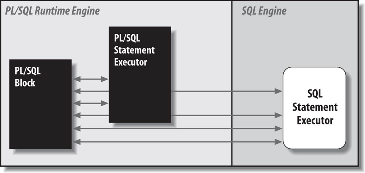
Figure 21-2. Context switching between PL/SQL and SQL

With FORALL and BULK COLLECT, however, you can fine-tune the way these two engines communicate, effectively telling the PL/SQL engine to compress multiple context switches into a single switch, thereby improving the performance of your applications.

Consider the FORALL statement shown in the figure. Rather than use a cursor FOR loop or a numeric loop to iterate through the rows to be updated, I use a FORALL header to specify a total number of iterations for execution. At runtime, the PL/SQL engine takes the “template” UPDATE statement and collection of bind variable values and generates them into a set of statements, which are then passed to the SQL engine with a single context switch. In other words, the same SQL statements are executed, but they are all run in the same roundtrip to the SQL layer, minimizing the context switches. This is shown in Figure 21-3.

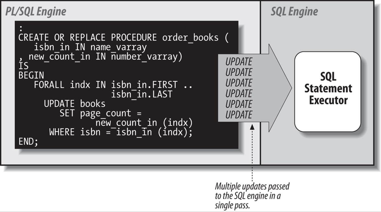
Figure 21-3. One context switch with FORALL

This reduction in context switches leads to a surprisingly sharp reduction in elapsed time for multirow SQL statements executed in PL/SQL. Let’s take a closer look at BULK COLLECT and FORALL.

High-Speed Querying with BULK COLLECT

With BULK COLLECT you can retrieve multiple rows of data through either an implicit or an explicit cursor with a single roundtrip to and from the database. BULK COLLECT reduces the number of context switches between the PL/SQL and SQL engines and thereby reduces the overhead of retrieving data.

Take a look at the following code snippet. I need to retrieve hundreds of rows of data on automobiles that have a poor environmental record. I place that data into a set of collections so that I can easily and quickly manipulate the data for both analysis and reporting:

DECLARE

TYPE names_t IS TABLE OF transportation.name%TYPE;

TYPE mileage_t IS TABLE OF transportation.mileage %TYPE;

names names_t := names_t();

mileages mileage_t := mileage_t();

CURSOR major_polluters_cur

IS

SELECT name, mileage FROM transportation

WHERE transport_type = 'AUTOMOBILE' AND mileage < 20;

BEGIN

FOR bad_car IN major_polluters_cur

LOOP

names.EXTEND;

names (major_polluters_cur%ROWCOUNT) := bad_car.NAME;

mileages.EXTEND;

mileages (major_polluters_cur%ROWCOUNT) := bad_car.mileage;

END LOOP;

-- Now work with data in the collections

END;

This certainly gets the job done, but the job might take a long time to complete. Consider this: if the transportation table contains 2,000 vehicles, then the PL/SQL engine issues 2,000 individual fetches against the cursor in the SGA.

To help out in this scenario, use the BULK COLLECT clause in the INTO element of your query. By using this clause in your cursor (explicit or implicit) you tell the SQL engine to bulk bind the output from the multiple rows fetched by the query into the specified collections before returning control to the PL/SQL engine. The syntax for this clause is:

... BULK COLLECT INTO collection_name[, collection_name] ...

where collection_name identifies a collection.

Here are some rules and restrictions to keep in mind when using BULK COLLECT:

§ You can use BULK COLLECT with both dynamic and static SQL.

§ You can use BULK COLLECT keywords in any of the following clauses: SELECT INTO, FETCH INTO, and RETURNING INTO.

§ The SQL engine automatically initializes and extends the collections you reference in the BULK COLLECT clause. It starts filling the collections at index 1, and inserts elements consecutively (densely).

§ SELECT...BULK COLLECT will not raise NO_DATA_FOUND if no rows are found. Instead, you must check the contents of the collection to see if there is any data inside it.

§ If the query returns no rows, the collection’s COUNT method will return 0.

Let’s explore these rules and the usefulness of BULK COLLECT through a series of examples. First, here is a rewrite of the major polluters example using BULK COLLECT:

DECLARE

TYPE names_t IS TABLE OF transportation.name%TYPE;

TYPE mileage_t IS TABLE OF transportation.mileage %TYPE;

names names_t;

mileages mileage_t;

BEGIN

SELECT name, mileage BULK COLLECT INTO names, mileages

FROM transportation

WHERE transport_type = 'AUTOMOBILE'

AND mileage < 20;

/* Now work with data in the collections */

END;

I am now able to remove the initialization and extension code from the row-by-row fetch implementation.

I don’t have to rely on implicit cursors to get this job done. Here is another reworking of the major polluters example, retaining the explicit cursor:

DECLARE

TYPE names_t IS TABLE OF transportation.name%TYPE;

TYPE mileage_t IS TABLE OF transportation.mileage %TYPE;

names names_t;

mileages mileage_t;

CURSOR major_polluters_cur IS

SELECT name, mileage FROM transportation

WHERE transport_type = 'AUTOMOBILE' AND mileage < 20;

BEGIN

OPEN major_polluters_cur;

FETCH major_polluters_cur BULK COLLECT INTO names, mileages;

CLOSE major_polluters_cur;

...

END;

I can also simplify my life and my code by fetching into a collection of records, as you see here:

DECLARE

TYPE transportation_aat IS TABLE OF transportation%ROWTYPE

INDEX BY PLS_INTEGER;

l_transportation transportation_aat;

BEGIN

SELECT * BULK COLLECT INTO l_transportation

FROM transportation

WHERE transport_type = 'AUTOMOBILE'

AND mileage < 20;

-- Now work with data in the collections

END;

NOTE

In Oracle Database 10g and later, the PL/SQL compiler will automatically optimize most cursor FOR loops so that they run with performance comparable to BULK COLLECT. You do not need to explicitly transform this code yourself—unless the body of your loop executes, directly or indirectly, DML statements. The database does not optimize DML statements into FORALL, so you will need to explicitly convert your cursor FOR loop to use BULK COLLECT. You can then use the collections populated by the BULK COLLECT to “drive” the FORALL statement.

Limiting rows retrieved with BULK COLLECT

Oracle provides a LIMIT clause for BULK COLLECT that allows you to limit the number of rows fetched from the database. The syntax is:

FETCH cursor BULK COLLECT INTO ... [LIMIT rows];

where rows can be any literal, variable, or expression that evaluates to an integer (otherwise, the database will raise a VALUE_ERROR exception).

LIMIT is very useful with BULK COLLECT, because it helps you manage how much memory your program will use to process data. Suppose, for example, that you need to query and process 10,000 rows of data. You could use BULK COLLECT to retrieve all those rows and populate a rather large collection. However, this approach will consume lots of memory in the PGA for that session. If this code is run by many separate Oracle schemas, your application’s performance may degrade because of PGA swapping.

The following block of code uses the LIMIT clause in a FETCH that is inside a simple loop:

DECLARE

CURSOR allrows_cur IS SELECT * FROM employees;

TYPE employee_aat IS TABLE OF allrows_cur%ROWTYPE

INDEX BY BINARY_INTEGER;

l_employees employee_aat;

BEGIN

OPEN allrows_cur;

LOOP

FETCH allrows_cur BULK COLLECT INTO l_employees LIMIT 100;

/* Process the data by scanning through the collection. */

FOR l_row IN 1 .. l_employees.COUNT

LOOP

upgrade_employee_status (l_employees(l_row).employee_id);

END LOOP;

EXIT WHEN allrows_cur%NOTFOUND;

END LOOP;

CLOSE allrows_cur;

END;

Notice that I terminate the loop by checking the value of allrows_cur%NOTFOUND at the bottom of the loop. When querying data one row at a time, I usually put this code immediately after the FETCH statement. You should not do that when using BULK COLLECT, because when the fetch retrieves the last set of rows, the cursor will be exhausted (and %NOTFOUND will return TRUE), but you will still have some elements in the collection to process.

So, either check the %NOTFOUND attribute at the bottom of your loop, or check the contents of the collection immediately after the fetch:

LOOP

FETCH allrows_cur BULK COLLECT INTO l_employees LIMIT 100;

EXIT WHEN l_employees.COUNT = 0;

The disadvantage of this second approach is that you will perform an extra fetch that returns no rows, compared to checking %NOTFOUND at the bottom of the loop body.

NOTE

Starting with Oracle Database 12c, you can also use the FIRST ROWS clause to limit the number of rows fetched with BULK COLLECT. The following block of code uses the LIMIT clause in a FETCH that is inside a simple loop. This code will retrieve just the first 50 rows identified by the SELECT statement:

DECLARE

TYPE salaries_t IS TABLE OF employees.salary%TYPE;

l_salaries salaries_t;

BEGIN

SELECT salary BULK COLLECT INTO sals FROM employees

FETCH FIRST 50 ROWS ONLY;

END;

/

Bulk fetching of multiple columns

As you have seen in previous examples, you certainly can bulk-fetch the contents of more than one column. It would be most elegant if you could fetch those multiple columns into a single collection of records. In fact, Oracle made this feature available starting with Oracle9i Database Release 2.

Suppose that I would like to retrieve all the information in my transportation table for each vehicle whose mileage is less than 20 miles per gallon. I can do so with a minimum of coding fuss:

DECLARE

-- Declare the type of collection

TYPE VehTab IS TABLE OF transportation%ROWTYPE;

-- Instantiate a particular collection from the TYPE

gas_guzzlers VehTab;

BEGIN

SELECT *

BULK COLLECT INTO gas_guzzlers

FROM transportation

WHERE mileage < 20;

...

Prior to Oracle9i Database Release 2, the preceding code would raise this exception:

PLS-00597: expression 'GAS_GUZZLERS' in the INTO list is of wrong type

You can use the LIMIT clause with a BULK COLLECT into a collection of records, just as you would with any other BULK COLLECT statement.

Using the RETURNING clause with bulk operations

You have now seen BULK COLLECT used for both implicit and explicit query cursors. You can also use BULK COLLECT inside a FORALL statement, in order to take advantage of the RETURNING clause.

The RETURNING clause allows you to obtain information (such as a newly updated value for a salary) from a DML statement. RETURNING can help you avoid additional queries to the database to determine the results of DML operations that have just completed.

Suppose that Congress has passed a law requiring that a company pay its highest-compensated employee no more than 50 times the salary of its lowest-paid employee. I work in the IT department of the newly merged company Northrop-Ford-Mattel-Yahoo-ATT, which employs a total of 250,000 workers. The word has come down from on high: the CEO is not taking a pay cut, so I need to increase the salaries of everyone who makes less than 50 times his 2013 total compensation package of $145 million—and decrease the salaries of all upper management except for the CEO. After all, somebody’s got to make up for this loss in profit!

Wow! I have lots of updating to do, and I want to use FORALL to get the job done as quickly as possible. However, I also need to perform various kinds of processing on the employee data and then print a report showing the change in salary for each affected employee. That RETURNING clause would come in awfully handy here, so let’s give it a try. (See the onlyfair.sql file on the book’s website for all of the steps shown here, plus table creation and INSERT statements.)

First, I’ll create a reusable function to return the compensation for an executive:

/* File on web: onlyfair.sql */

FUNCTION salforexec (title_in IN VARCHAR2) RETURN NUMBER

IS

CURSOR ceo_compensation IS

SELECT salary + bonus + stock_options +

mercedes_benz_allowance + yacht_allowance

FROM compensation

WHERE title = title_in;

big_bucks NUMBER;

BEGIN

OPEN ceo_compensation;

FETCH ceo_compensation INTO big_bucks;

RETURN big_bucks;

END;

In the main block of the update program, I declare a number of local variables and the following query to identify underpaid employees and overpaid employees who are not lucky enough to be the CEO:

DECLARE

big_bucks NUMBER := salforexec ('CEO');

min_sal NUMBER := big_bucks / 50;

names name_tab;

old_salaries number_tab;

new_salaries number_tab;

CURSOR affected_employees (ceosal IN NUMBER)

IS

SELECT name, salary + bonus old_salary

FROM compensation

WHERE title != 'CEO'

AND ((salary + bonus < ceosal / 50)

OR (salary + bonus > ceosal / 10)) ;

At the start of my executable section, I load all of this data into my collections with a BULK COLLECT query:

OPEN affected_employees (big_bucks);

FETCH affected_employees

BULK COLLECT INTO names, old_salaries;

Then I can use the names collection in my FORALL update:

FORALL indx IN names.FIRST .. names.L*

UPDATE compensation

SET salary =

GREATEST(

DECODE (

GREATEST (min_sal, salary),

min_sal, min_sal,

salary / 5),

min_sal )

WHERE name = names (indx)

RETURNING salary BULK COLLECT INTO new_salaries;

I use DECODE to give an employee either a major boost in yearly income or an 80% cut in pay to keep the CEO comfy. I end it with a RETURNING clause that relies on BULK COLLECT to populate a third collection: the new salaries.

Finally, because I used RETURNING and don’t have to write another query against the compensation table to obtain the new salaries, I can immediately move to report generation:

FOR indx IN names.FIRST .. names.LAST

LOOP

DBMS_OUTPUT.PUT_LINE (

RPAD (names(indx), 20) ||

RPAD (' Old: ' || old_salaries(indx), 15) ||

' New: ' || new_salaries(indx)

);

END LOOP;

Here, then, is the report generated from the onlyfair.sql script:

John DayAndNight Old: 10500 New: 2900000

Holly Cubicle Old: 52000 New: 2900000

Sandra Watchthebucks Old: 22000000 New: 4000000

Now everyone can afford quality housing and health care. And tax revenue at all levels will increase, so public schools can get the funding they need.

NOTE

The RETURNING column values or expressions returned by each execution in FORALL are added to the collection after the values returned previously. If you use RETURNING inside a nonbulk FOR loop, previous values are overwritten by the latest DML execution.

High-Speed DML with FORALL

BULK COLLECT speeds up queries. FORALL does the same thing for inserts, updates, deletes, and merges (FORALL with a merge is supported in only Oracle Database 11g and later); I will refer to these statements collectively as “DML.” FORALL tells the PL/SQL runtime engine to bulk bind into the SQL statement all of the elements of one or more collections before sending its statements to the SQL engine.

Given the centrality of SQL to Oracle-based applications and the heavy impact of DML statements on overall performance, FORALL is probably the single most important optimization feature in the PL/SQL language.

So, if you are not yet using FORALL, I have bad news and good news. The bad news is that your application’s code base has not been enhanced over the years to take advantage of critical Oracle features. The good news is that when you do start using it, your users will experience some very pleasant (and relatively easy to achieve) boosts in performance.

You will find in the following pages explanations of all of the features and nuances of FORALL, along with plenty of examples.

Syntax of the FORALL statement

Although the FORALL statement contains an iteration scheme (i.e., it iterates through all the rows of a collection), it is not a FOR loop. Consequently, it has neither a LOOP nor an END LOOP statement. Its syntax is as follows:

FORALL index IN

[ lower_bound ... upper_bound |

INDICES OF indexing_collection |

VALUES OF indexing_collection

]

[ SAVE EXCEPTIONS ]

sql_statement;

where:

index

Is an integer, declared implicitly by Oracle, that is a defined index value in the collection

lower_bound

Is the starting index value (row or collection element) for the operation

upper_bound

Is the ending index value (row or collection element) for the operation

sql_statement

Is the SQL statement to be performed on each collection element

indexing_collection

Is the PL/SQL collection used to select the indices in the bind array referenced in the sql_statement; the INDICES OF and VALUES_OF alternatives are available starting in Oracle Database 10g

SAVE EXCEPTIONS

Is an optional clause that tells FORALL to process all rows, saving any exceptions that occur

You must follow these rules when using FORALL:

§ The body of the FORALL statement must be a single DML statement—an INSERT, UPDATE, DELETE, or MERGE (in Oracle Database 11g and later).

§ The DML statement must reference collection elements, indexed by the index_row variable in the FORALL statement. The scope of the index_row variable is the FORALL statement only; you may not reference it outside of that statement. Note, though, that the upper and lower bounds of these collections do not have to span the entire contents of the collection(s).

§ Do not declare a variable for index_row. It is declared implicitly as PLS_INTEGER by the PL/SQL engine.

§ The lower and upper bounds must specify a valid range of consecutive index numbers for the collection(s) referenced in the SQL statement. Sparsely filled collections will raise the following error:

ORA-22160: element at index [3] does not exist

See the missing_element.sql file on the book’s website for an example of this scenario.

Starting with Oracle Database 10g, you can use the INDICES OF and VALUES OF syntax to allow use of sparse collections (where there are undefined elements between FIRST and LAST). These clauses are covered later in this chapter.

§ Until Oracle Database 11g, fields within collections of records could not be referenced within the DML statement. Instead, you could only reference the row in the collection as a whole, whether the fields were collections of scalars or collections of more complex objects. For example, the following code:

§ DECLARE

§ TYPE employee_aat IS TABLE OF employees%ROWTYPE

§ INDEX BY PLS_INTEGER;

§ l_employees employee_aat;

§ BEGIN

§ FORALL l_index IN l_employees.FIRST .. l_employees.LAST

§ INSERT INTO employee (employee_id, last_name)

§ VALUES (l_employees (l_index).employee_id

§ , l_employees (l_index).last_name

§ );

END;

will cause the following compilation error in releases prior to Oracle Database 11g:

PLS-00436: implementation restriction: cannot reference fields

of BULK In-BIND table of records

To use FORALL in this case, you would need to load the employee IDs and the last names into two separate collections. Thankfully, this restriction was removed in Oracle Database 11g.

§ The collection subscript referenced in the DML statement cannot be an expression. For example, the following script:

§ DECLARE

§ names name_varray := name_varray ();

§ BEGIN

§ FORALL indx IN names.FIRST .. names.LAST

§ DELETE FROM emp WHERE ename = names(indx+10);

END;

will cause the following error:

PLS-00430: FORALL iteration variable INDX is not allowed in this context

FORALL examples

Here are some examples of the use of the FORALL statement:

§ Change the page count of all books whose ISBNs appear in the isbns_in collection:

§ PROCEDURE order_books (

§ isbns_in IN name_varray,

§ new_counts_in IN number_varray)

§ IS

§ BEGIN

§ FORALL indx IN isbns_in.FIRST .. isbns_in.LAST

§ UPDATE books

§ SET page_count = new_counts_in (indx)

§ WHERE isbn = isbns_in (indx);

END;

Notice that the only changes from a typical FOR loop in this example are to change FOR to FORALL, and to remove the LOOP and END LOOP keywords. This use of FORALL accesses and passes to SQL each of the rows defined in the two collections. Refer back to Figure 21-3 for the change in behavior that results.

§ Reference more than one collection from a DML statement. In this case, I have three collections: denial, patient_name, and illnesses. Only the first two are subscripted, resulting in individual elements of these collections being passed to each INSERT. The third column in health_coverage is a collection listing preconditions. Because the PL/SQL engine bulk binds only subscripted collections, the entire illnesses collection is placed in that column for each row inserted:

§ FORALL indx IN denial.FIRST .. denial.LAST

§ INSERT INTO health_coverage

VALUES (denial(indx), patient_name(indx), illnesses);

§ Use the RETURNING clause in a FORALL statement to retrieve information about each separate DELETE statement. Notice that the RETURNING clause in FORALL must use BULK COLLECT INTO (the corresponding “bulk” operation for queries):

§ FUNCTION remove_emps_by_dept (deptlist IN dlist_t)

§ RETURN enolist_t

§ IS

§ enolist enolist_t;

§ BEGIN

§ FORALL aDept IN deptlist.FIRST..deptlist.LAST

§ DELETE FROM employees WHERE department_id IN deptlist(aDept)

§ RETURNING employee_id BULK COLLECT INTO enolist;

§ RETURN enolist;

END;

§ Use the indices defined in one collection to determine which rows in the binding array (the collection referenced inside the SQL statement) will be used in the dynamic INSERT:

§ FORALL indx IN INDICES OF l_top_employees

§ EXECUTE IMMEDIATE

§ 'INSERT INTO ' || l_table || ' VALUES (:emp_pky, :new_salary)'

§ USING l_new_salaries(indx).employee_id,

l_new_salaries(indx).salary;

Cursor attributes for FORALL

You can use cursor attributes after you execute a FORALL statement to get information about the DML operation run within FORALL. Oracle also offers an additional attribute, %BULK_ROWCOUNT, to give you more granular information about the results of the bulk DML statement.

Table 21-1 describes the significance of the values returned by these attributes for FORALL.

Table 21-1. Implicit SQL cursor attributes for FORALL statements

Let’s now explore the %BULK_ROWCOUNT composite attribute. This attribute, designed specifically for use with FORALL, has the semantics of (acts like) an associative array or collection. The database deposits in the Nth element in this collection the number of rows processed by theNth execution of the FORALL’s INSERT, UPDATE, DELETE, or MERGE. If no rows were affected, the Nth row will contain a zero value.

Here is an example of using %BULK_ROWCOUNT (and the overall %ROWCOUNT attribute as well):

DECLARE

TYPE isbn_list IS TABLE OF VARCHAR2(13);

my_books isbn_list

:= isbn_list (

'1-56592-375-8', '0-596-00121-5', '1-56592-849-0',

'1-56592-335-9', '1-56592-674-9', '1-56592-675-7',

'0-596-00180-0', '1-56592-457-6'

);

BEGIN

FORALL book_index IN

my_books.FIRST..my_books.LAST

UPDATE books

SET page_count = page_count / 2

WHERE isbn = my_books (book_index);

-- Did I update the total number of books I expected?

IF SQL%ROWCOUNT != 8

THEN

DBMS_OUTPUT.PUT_LINE (

'We are missing a book!');

END IF;

-- Did the 4th UPDATE statement affect any rows?

IF SQL%BULK_ROWCOUNT(4) = 0

THEN

DBMS_OUTPUT.PUT_LINE (

'What happened to Oracle PL/SQL Programming?');

END IF;

END;

Here are some tips on how this attribute works:

§ The FORALL statement and %BULK_ROWCOUNT use the same subscripts or row numbers in the collections. For example, if the collection passed to FORALL has data in rows 10 through 200, then the %BULK_ROWCOUNT pseudocollection will also have rows 10 through 200 defined and populated. Any other rows will be undefined.

§ When the INSERT affects only a single row (when you specify a VALUES list, for example), a row’s value in %BULK_ROWCOUNT will be equal to 1. For INSERT...SELECT statements, however, %BULK_ROWCOUNT can be greater than 1.

§ The value in a row of the %BULK_ROWCOUNT pseudoarray for deletes, updates, and insert-selects may be any natural number (0 or positive); these statements can modify more than one row, depending on their WHERE clauses.

ROLLBACK behavior with FORALL

The FORALL statement allows you to pass multiple SQL statements all together (in bulk) to the SQL engine. This means that you have a single context switch—but each statement still executes separately in the SQL engine.

What happens when one of those DML statements fails?

1. The DML statement that raised the exception is rolled back to an implicit savepoint marked by the PL/SQL engine before execution of the statement. Changes to all rows already modified by that statement are rolled back.

2. Any previous DML operations in that FORALL statement that have already completed without error are not rolled back.

3. If you do not take special action (by adding the SAVE EXCEPTIONS clause to FORALL, discussed next), the entire FORALL statement stops and the remaining statements are not executed at all.

Continuing past exceptions with SAVE EXCEPTIONS

By adding the SAVE EXCEPTIONS clause to your FORALL header, you instruct the Oracle database to continue processing even when an error has occurred. The database will then “save the exception” (or multiple exceptions, if more than one error occurs). When the DML statement completes, it will then raise the ORA-24381 exception. In the exception section, you can then access a pseudocollection called SQL%BULK_EXCEPTIONS to obtain error information.

Here is an example, followed by an explanation of what is going on:

/* File on web: bulkexc.sql */

1 DECLARE

2 bulk_errors EXCEPTION;

3 PRAGMA EXCEPTION_INIT (bulk_errors, −24381);

4 TYPE namelist_t IS TABLE OF VARCHAR2(32767);

5

6 enames_with_errors namelist_t

7 := namelist_t ('ABC',

8 'DEF',

9 NULL, /* Last name cannot be NULL */

10 'LITTLE',

11 RPAD ('BIGBIGGERBIGGEST', 250, 'ABC'), /* Value too long */

12 'SMITHIE'

13 );

14 BEGIN

15 FORALL indx IN enames_with_errors.FIRST .. enames_with_errors.LAST

16 SAVE EXCEPTIONS

17 UPDATE EMPLOYEES

18 SET last_name = enames_with_errors (indx);

19

20 EXCEPTION

21 WHEN bulk_errors

22 THEN

23 DBMS_OUTPUT.put_line ('Updated ' || SQL%ROWCOUNT || ' rows.');

24

25 FOR indx IN 1 .. SQL%BULK_EXCEPTIONS.COUNT

26 LOOP

27 DBMS_OUTPUT.PUT_LINE ('Error '

28 || indx

29 || ' occurred during '

30 || 'iteration '

31 || SQL%BULK_EXCEPTIONS (indx).ERROR_INDEX

32 || ' updating name to '

33 || enames_with_errors (SQL%BULK_EXCEPTIONS (indx).ERROR_INDEX);

34 DBMS_OUTPUT.PUT_LINE ('Oracle error is '

35 || SQLERRM ( −1 * SQL%BULK_EXCEPTIONS (indx).ERROR_CODE)

36 );

37 END LOOP;

38 END;

When I run this code with SERVEROUTPUT turned on, I see these results:

SQL> EXEC bulk_exceptions

Error 1 occurred during iteration 3 updating name to BIGBIGGERBIGGEST

Oracle error is ORA-01407: cannot update () to NULL

Error 2 occurred during iteration 5 updating name to

Oracle error is ORA-01401: inserted value too large for column

In other words, the database encountered two exceptions as it processed the DML for the names collection. It did not stop with the first exception, but continued on, cataloging a second.

The following table describes the error-handling functionality in this code.

Driving FORALL with nonsequential arrays

Prior to Oracle Database 10g, the collection referenced inside the FORALL statement (the “binding array”) had to be densely or consecutively filled. In code such as the following, if there were any gaps between the low and high values specified in the range of the FORALL header Oracle would raise an error:

1 DECLARE

2 TYPE employee_aat IS TABLE OF employees.employee_id%TYPE

3 INDEX BY PLS_INTEGER;

4 l_employees employee_aat;

5 BEGIN

6 l_employees (1) := 100;

7 l_employees (100) := 1000;

8 FORALL l_index IN l_employees.FIRST .. l_employees.LAST

9 UPDATE employees SET salary = 10000

10 WHERE employee_id = l_employees (l_index);

11 END;

12 /

The error message looked like this:

DECLARE

*

ERROR at line 1:

ORA-22160: element at index [2] does not exist

Furthermore, there was no way for you to skip over rows in the binding array that you didn’t want processed by the FORALL statement. These restrictions often led to the writing of additional code to compress collections to fit the limitations of FORALL. To help PL/SQL developers avoid this nuisance coding, starting with Oracle Database 10g PL/SQL offers the INDICES OF and VALUES OF clauses, both of which allow you to specify the portion of the binding array to be processed by FORALL.

First let’s review the difference between these two clauses, and then I will explore examples to demonstrate their usefulness:

INDICES OF

Use this clause when you have a collection (let’s call it the indexing array) whose defined rows specify which rows in the binding array (referenced inside the FORALL’s DML statement) you would like to be processed. In other words, if the element at position N (a.k.a. the row number) is not defined in the indexing array, you want the FORALL statement to ignore the element at position N in the binding array.

VALUES OF

Use this clause when you have a collection of integers (again, the indexing array) whose content (the value of the element at a specified position) identifies the position in the binding array that you want to be processed by the FORALL statement.

INDICES OF example

I would like to update the salaries of some employees to $10,000. Currently, no one has such a salary:

SQL> SELECT employee_id FROM employees WHERE salary = 10000;

no rows selected

I then write the following program:

/* File on web: 10g_indices_of.sql */

1 DECLARE

2 TYPE employee_aat IS TABLE OF employees.employee_id%TYPE

3 INDEX BY PLS_INTEGER;

4

5 l_employees employee_aat;

6

7 TYPE boolean_aat IS TABLE OF BOOLEAN

8 INDEX BY PLS_INTEGER;

9

10 l_employee_indices boolean_aat;

11 BEGIN

12 l_employees (1) := 7839;

13 l_employees (100) := 7654;

14 l_employees (500) := 7950;

15 --

16 l_employee_indices (1) := TRUE;

17 l_employee_indices (500) := TRUE;

18 l_employee_indices (799) := TRUE;

19

20 FORALL l_index IN INDICES OF l_employee_indices

21 BETWEEN 1 AND 500

22 UPDATE employees23 SET salary = 10000

24 WHERE employee_id = l_employees (l_index);

25 END;

The following table describes the logic of the program.

After executing this code, I query the table to see that, in fact, only two rows of the table were updated—the employee with ID 7654 was skipped because the Boolean indices collection had no element defined at position 100:

SQL> SELECT employee_id FROM employee WHERE salary = 10000;

EMPLOYEE_ID

-----------

7839

7950

With INDICES OF (line 20), the contents of the indexing array are ignored. All that matters are the positions or row numbers that are defined in the collection.

VALUES OF example

Again, I would like to update the salaries of some employees to $10,000, this time using the VALUES OF clause. Currently, no one has such a salary:

SQL> SELECT employee_id FROM employee WHERE salary = 10000;

no rows selected

I then write the following program:

/* File on web: 10g_values_of.sql */

1 DECLARE

2 TYPE employee_aat IS TABLE OF employees.employee_id%TYPE

3 INDEX BY PLS_INTEGER;

4

5 l_employees employee_aat;

6

7 TYPE indices_aat IS TABLE OF PLS_INTEGER

8 INDEX BY PLS_INTEGER;

9

10 l_employee_indices indices_aat;

11 BEGIN

12 l_employees (-77) := 7820;

13 l_employees (13067) := 7799;

14 l_employees (99999999) := 7369;

15 --

16 l_employee_indices (100) := −77;

17 l_employee_indices (200) := 99999999;

18 --

19 FORALL l_index IN VALUES OF l_employee_indices

20 UPDATE employees

21 SET salary = 10000

22 WHERE employee_id = l_employees (l_index);

23 END;

The following table describes the logic of the program.

After executing this code, I query the table to see that again only two rows of the table were updated—the employee with ID 7799 was skipped because the “values of” collection had no element whose value equaled 13067:

SQL> SELECT employee_id FROM employees WHERE salary = 10000;

EMPLOYEE_ID

-----------

7369

7820

Improving Performance with Pipelined Table Functions

Pipelined functions are where the elegance and simplicity of PL/SQL converge with the performance of SQL. Complex data transformations are effortless to develop and support with PL/SQL, yet to achieve high-performance data processing, we often resort to set-based SQL solutions. Pipelined functions bridge the gap between the two methods effortlessly, but they also have some unique performance features of their own, making them a superb performance optimization tool.

In the following pages, I’ll show some examples of typical data-processing requirements and how you might tune them with pipelined functions. I’ll cover the following topics:

§ How to tune typical data-loading requirements with pipelined functions. In each case, I’ll convert legacy row-based solutions to set-based solutions that include parallel pipelined functions.

§ How to exploit the parallel context of pipelined functions to improve the performance of data unloads.

§ The relative performance of the partitioning and streaming options for parallel pipelined functions.

§ How the cost-based optimizer (CBO) deals with both pipelined and standard table functions.

§ How complex multitable loading requirements can be solved with multitype pipelined functions.

The basic syntax for pipelined table functions was covered in Chapter 17. To recap, a pipelined function is called in the FROM clause of a SQL statement and is queried as if it were a relational table or other rowsource. Unlike standard table functions (that have to complete all of their processing before passing a potentially large collection of data back to the calling context), pipelined table functions stream their results to the client almost as soon as they are prepared. In other words, pipelined functions do not materialize their entire result set, and this optimization feature dramatically reduces their PGA memory footprint. Another unique performance feature of pipelined functions is the ability to call them in the context of a parallel query. I have taken advantage of these unique performance features many times, and in the next few pages I will show you how and when to use pipelined functions to improve the performance of some of your own programs.

Replacing Row-Based Inserts with Pipelined Function-Based Loads

To demonstrate the performance of pipelined functions, let’s first imagine a typical legacy loading scenario that I want to bring into the 21st century. Using the stockpivot example, I have coded a simple row-by-row load to fetch the stockpivot source data and pivot each record into two rows for insertion. It is contained in a package and is as follows:

/* File on web: stockpivot_setup.sql */

PROCEDURE load_stocks_legacy IS

CURSOR c_source_data IS

SELECT ticker, open_price, close_price, trade_date

FROM stocktable;

r_source_data stockpivot_pkg.stocktable_rt;

r_target_data stockpivot_pkg.tickertable_rt;

BEGIN

OPEN c_source_data;

LOOP

FETCH c_source_data INTO r_source_data;

EXIT WHEN c_source_data%NOTFOUND;

/* Opening price... */

r_target_data.ticker := r_source_data.ticker;

r_target_data.price_type := 'O';

r_target_data.price := r_source_data.open_price;

r_target_data.price_date := r_source_data.trade_date;

INSERT INTO tickertable VALUES r_target_data;

/* Closing price... */

r_target_data.price_type := 'C';

r_target_data.price := r_source_data.close_price;

INSERT INTO tickertable VALUES r_target_data;

END LOOP;

CLOSE c_source_data;

END load_stocks_legacy;

I regularly see code of this format, and since Oracle8i Database I’ve typically used BULK COLLECT and FORALL as my primary tuning tool (when the logic is too complex for a set-based SQL solution). However, an alternative technique (that I first saw described by Tom Kyte^[19^]) is to use a set-based insert from a pipelined function. In other words, a pipelined function is used for all of the legacy data transformation and preparation logic, but the target-table load is handled separately as a set-based insert. Since reading about this powerful technique, I have used it successfully in my own performance optimization work, as described in the following sections.

A pipelined function implementation

As demonstrated in Chapter 17, the first thing to consider when creating a pipelined function is the data that it will return. For this, I need to create an object type to define a single row of the pipelined function’s return data:

/* File on web: stockpivot_setup.sql */

CREATE TYPE stockpivot_ot AS OBJECT

( ticker VARCHAR2(10)

, price_type VARCHAR2(1)

, price NUMBER

, price_date DATE

);

I also need to create a collection of this object, as this defines the function’s return type:

/* File on web: stockpivot_setup.sql */

CREATE TYPE stockpivot_ntt AS TABLE OF stockpivot_ot;

Transforming the legacy code into a pipelined function is quite simple. First I must define the function specification in the header. I must also include a load procedure that I will describe later:

/* File on web: stockpivot_setup.sql */

CREATE PACKAGE stockpivot_pkg AS

TYPE stocktable_rct IS REF CURSOR

RETURN stocktable%ROWTYPE;

<snip>

FUNCTION pipe_stocks(

p_source_data IN stockpivot_pkg.stocktable_rct

) RETURN stockpivot_ntt PIPELINED;

PROCEDURE load_stocks;

END stockpivot_pkg;

My pipelined function takes a strong REF CURSOR as an input parameter (I could also use a weak REF CURSOR in this case). The cursor parameter itself is not necessarily required. It would be just as valid for me to declare the cursor in the function itself (as I did with the legacy procedure). However, the cursor parameter is going to be required for further iterations of this pipelined function, so I’ve introduced it from the outset.

The function’s implementation follows:

/* File on web: stockpivot_setup.sql */

1 FUNCTION pipe_stocks(

2 p_source_data IN stockpivot_pkg.stocktable_rct

3 ) RETURN stockpivot_ntt PIPELINED IS

4

5 r_target_data stockpivot_ot := stockpivot_ot(NULL, NULL, NULL, NULL);

6 r_source_data stockpivot_pkg.stocktable_rt;

7

8 BEGIN

9 LOOP

10 FETCH p_source_data INTO r_source_data;

11 EXIT WHEN p_source_data%NOTFOUND;

12

13 /* First row... */

14 r_target_data.ticker := r_source_data.ticker;

15 r_target_data.price_type := 'O';

16 r_target_data.price := r_source_data.open_price;

17 r_target_data.price_date := r_source_data.trade_date;

18 PIPE ROW (r_target_data);

19

20 /* Second row... */

21 r_target_data.price_type := 'C';

22 r_target_data.price := r_source_data.close_price;

23 PIPE ROW (r_target_data);

24

25 END LOOP;

26 CLOSE p_source_data;

27 RETURN;

28 END pipe_stocks;

Other than the general pipelined function syntax (that you should by now be familiar with from Chapter 17), the majority of the pipelined function’s code is recognizable from the legacy example. The main differences to consider are summarized in the following table.

Loading from a pipelined function

As you can see, with only a small number of changes to the original load program, I now have a pipelined function that prepares and pipes all of the data that I need to load into tickertable. To complete the conversion of my legacy code, I only need to write an additional procedure to insert the piped data into my target table:

/* File on web: stockpivot_setup.sql */

PROCEDURE load_stocks IS

BEGIN

INSERT INTO tickertable (ticker, price_type, price, price_date)

SELECT ticker, price_type, price, price_date

FROM TABLE(

stockpivot_pkg.pipe_stocks(

CURSOR(SELECT * FROM stocktable)));

END load_stocks;

That completes the basic conversion of the row-by-row legacy code to a pipelined function solution. So how does this compare to the original? In my tests, I created the stocktable as an external table with a file of 500,000 records. The legacy row-by-row code completed in 57 seconds (inserting 1 million rows into tickertable), and the set-based insert using the pipelined function ran in just 16 seconds (test results for all examples are available on the book’s website).

Considering that this is my first and most basic pipelined function implementation, the improvement in performance just shown is quite respectable. However, it is not quite the performance I can get when using a simple BULK COLLECT and FORALL solution (which runs in just over 5 seconds in my tests), so I will need to make some modifications to my pipelined function load.

Before I do this, however, notice that I retained the single-row fetches off the main cursor and did nothing to reduce the “expensive” context switching (which would require a BULK COLLECT fetch). So why is it faster than the legacy row-by-row code?

It is faster primarily because of the switch to set-based SQL. Set-based DML (such as the INSERT...SELECT I used in my pipelined load) is almost always considerably faster than a row-based, procedural solution. In this particular case, I have benefited directly from the Oracle database’s internal optimization of set-based inserts. Specifically, the database writes considerably less redo information for set-based inserts (INSERT...SELECT) than it does for singleton inserts (INSERT...VALUES). That is to say, if I insert 100 rows in a single statement, it will generate less redo information than if I inserted 100 rows one by one.

My original legacy load of 1 million tickertable rows generated over 270 MB of redo information. This was reduced to just over 37 MB when I used the pipelined function-based load, contributing to a significant proportion of the time savings.

NOTE

I have omitted any complicated data transformations from my examples for the sake of clarity. You should assume in all cases that the data-processing rules are sufficiently complex to warrant a PL/SQL pipelined function solution in the first place. Otherwise, I would probably just use a set-based SQL solution with analytic functions, subquery factoring, and CASE expressions to transform my high-volume data!

Tuning pipelined functions with array fetches

Despite having tuned the legacy code with a pipelined function implementation, I am not done yet. There are further optimization possibilities, and I need to make my processing at least as fast as a BULK COLLECT and FORALL solution. Notice that I used single-row fetches from the main source cursor. The first simple tuning possibility is therefore to use array fetches with BULK COLLECT.

I begin by adding a default array size to my package specification. The optimal array fetch size will vary according to your specific data-processing requirements, but I always prefer to start my tests with 100 and work from there. I also add an associative array type to the package specification (it could just as well be declared in the body); this is for bulk fetches from the source cursor. Finally, I add a second parameter to the pipelined function signature so that I can control the array fetch size (this isn’t necessary, of course—just good practice). My specification is now as follows:

/* File on web: stockpivot_setup.sql */

CREATE PACKAGE stockpivot_pkg AS

<snip>

c_default_limit CONSTANT PLS_INTEGER := 100;

TYPE stocktable_aat IS TABLE OF stocktable%ROWTYPE

INDEX BY PLS_INTEGER;

FUNCTION pipe_stocks_array(

p_source_data IN stockpivot_pkg.stocktable_rct,

p_limit_size IN PLS_INTEGER DEFAULT stockpivot_pkg.c_default_limit

) RETURN stockpivot_ntt PIPELINED;

<snip>

END stockpivot_pkg;

The function itself is very similar to the original version:

/* File on web: stockpivot_setup.sql */

FUNCTION pipe_stocks_array(

p_source_data IN stockpivot_pkg.stocktable_rct,

p_limit_size IN PLS_INTEGER DEFAULT stockpivot_pkg.c_default_limit

) RETURN stockpivot_ntt PIPELINED IS

r_target_data stockpivot_ot := stockpivot_ot(NULL, NULL, NULL, NULL);

aa_source_data stockpivot_pkg.stocktable_aat;

BEGIN

LOOP

FETCH p_source_data BULK COLLECT INTO aa_source_data LIMIT p_limit_size;

EXIT WHEN aa_source_data.COUNT = 0;

/* Process the batch of (p_limit_size) records... */

FOR i IN 1 .. aa_source_data.COUNT LOOP

/* First row... */

r_target_data.ticker := aa_source_data(i).ticker;

r_target_data.price_type := 'O';

r_target_data.price := aa_source_data(i).open_price;

r_target_data.price_date := aa_source_data(i).trade_date;

PIPE ROW (r_target_data);

/* Second row... */

r_target_data.price_type := 'C';

r_target_data.price := aa_source_data(i).close_price;

PIPE ROW (r_target_data);

END LOOP;

END LOOP;

CLOSE p_source_data;

RETURN;

END pipe_stocks_array;

The only difference from my original version is the use of BULK COLLECT...LIMIT from the source cursor. The load procedure is the same as before, modified to reference the array version of the pipelined function. This reduced my loading time further to just 6 seconds, purely because of the reduction in context switching from array-based PL/SQL. My pipelined function solution now has comparable performance to my BULK COLLECT and FORALL solution.

Exploiting parallel pipelined functions for ultimate performance

I’ve achieved some good performance gains from the switch to a set-based insert from a pipelined function. Yet I have one more tuning option for my stockpivot load that will give me better performance than any other solution: using the parallel capability of pipelined functions described inChapter 17. In this next iteration, I parallel enable my stockpivot function by adding another clause to the function signature:

/* File on web: stockpivot_setup.sql */

CREATE PACKAGE stockpivot_pkg AS

<snip>

FUNCTION pipe_stocks_parallel(

p_source_data IN stockpivot_pkg.stocktable_rct

p_limit_size IN PLS_INTEGER DEFAULT stockpivot_pkg.c_default_limit

) RETURN stockpivot_ntt

PIPELINED

PARALLEL_ENABLE (PARTITION p_source_data BY ANY);

<snip>

END stockpivot_pkg;

By using the ANY partitioning scheme, I have instructed the Oracle database to randomly allocate my source data to the parallel processes. This is because the order in which the function receives and processes the source data has no effect on the resulting output (i.e., there are no inter-row dependencies). That is not always the case, of course.

Enabling parallel pipelined function execution

Aside from the parallel-enabling syntax in the specification and body, the function implementation is the same as the array-fetch example (see the stockpivot_setup.sql file on the website for the full package). However, I need to ensure that my tickertable load is executed in parallel. First, I must enable parallel DML at the session level. Once this is done, I invoke parallel query in one of the following ways:

§ Using the PARALLEL hint

§ Using parallel DEGREE settings on the underlying objects

§ Forcing parallel query (ALTER SESSION FORCE PARALLEL (QUERY) PARALLEL n)

NOTE

Parallel query/DML is a feature of Oracle Database Enterprise Edition. If you’re using either Standard Edition or Standard Edition One, you are not licensed to use the parallel feature of pipelined functions.

In my load, I have enabled parallel DML at the session level and used hints to specify a degree of parallelism (DOP) of 4:

/* File on web: stockpivot_setup.sql */

PROCEDURE load_stocks_parallel IS

BEGIN

EXECUTE IMMEDIATE 'ALTER SESSION ENABLE PARALLEL DML';

INSERT /*+ PARALLEL(t, 4) */ INTO tickertable t

(ticker, price_type, price, price_date)

SELECT ticker, price_type, price, price_date

FROM TABLE(

stockpivot_pkg.pipe_stocks_parallel(

CURSOR(SELECT /*+ PARALLEL(s, 4) */ * FROM stocktable s)));

END load_stocks_parallel;

This reduces the load time to just over 3 seconds, a significant improvement on my original legacy code and all other versions of my pipelined function load. Of course, when we’re dealing in small units of time such as this, the startup costs of parallel processes will impact the overall runtime, but I have still managed almost a 50% improvement on my array version. The fact that parallel inserts use direct path loads rather than conventional path loads also means that the redo generation dropped further still, to just 25 KB!

In commercial systems you might be tuning processes that run for an hour or more, so the gains you can achieve with parallel pipelined loads will be significant in both proportional and actual terms.

NOTE

When you are using parallel pipelined functions, your source cursor must be passed as a REF CURSOR parameter. In serial pipelined functions, the source cursor can be embedded in the function itself (although I have chosen not to do this in any of my examples).

Furthermore, the REF CURSOR can be either weakly or strongly typed for functions partitioned with the ANY scheme, but for HASH- or RANGE-based partitioning, it must be strongly typed. See Chapter 15 for more details on REF CURSORs and cursor variables.

Tuning Merge Operations with Pipelined Functions

You might now be considering serial or parallel pipelined functions as a tuning mechanism for your own high-volume data loads. Yet not all loads involve inserts like the stockpivot example. Many data loads are incremental and require periodic merges of new and modified data. The good news is that the same principle of combining PL/SQL transformations with set-based SQL applies to merges (and updates) as well.

Row-based PL/SQL merge processing

Consider the following procedure, taken from my employee_pkg example. I have a merge of a large number of employee records, but my legacy code uses an old PL/SQL technique of attempting an update first and inserting only when the update matches zero records in the target table:

/* File on web: employees_merge_setup.sql */

PROCEDURE upsert_employees IS

n PLS_INTEGER := 0;

BEGIN

FOR r_emp IN (SELECT * FROM employees_staging) LOOP

UPDATE employees

SET <snip>

WHERE employee_id = r_emp.employee_id;

IF SQL%ROWCOUNT = 0 THEN

INSERT INTO employees (<snip>)

VALUES (<snip>);

END IF;

END LOOP;

END upsert_employees;

I’ve removed some of the code for brevity, but you can clearly see the “upsert” technique in action. Note that I’ve used an implicit cursor FOR loop that will benefit from the array-fetch optimization introduced to PL/SQL in Oracle Database 10g.

To test this procedure, I created a staging table of 500,000 employee records (this is a massive corporation!) and inserted 250,000 of them into an employees table to manufacture an even split between updates and inserts. This PL/SQL “poor man’s merge” solution completed in 46 seconds.

Using pipelined functions for set-based MERGE

Converting this example to a set-based SQL MERGE from a pipelined function is, once again, quite simple. First, I create the supporting object and nested table types (see the employees_merge_setup.sql file for details) and declare the function in the package header:

/* File on web: employees_merge_setup.sql */

CREATE PACKAGE employee_pkg AS

c_default_limit CONSTANT PLS_INTEGER := 100;

TYPE employee_rct IS REF CURSOR RETURN employees_staging%ROWTYPE;

TYPE employee_aat IS TABLE OF employees_staging%ROWTYPE

INDEX BY PLS_INTEGER;

<snip>

FUNCTION pipe_employees(

p_source_data IN employee_pkg.employee_rct

p_limit_size IN PLS_INTEGER DEFAULT employee_pkg.c_default_limit

) RETURN employee_ntt

PIPELINED

PARALLEL_ENABLE (PARTITION p_source_data BY ANY);

END employee_pkg;

I have parallel enabled the pipelined function and used the ANY partitioning scheme, as before. The function implementation is as follows:

/* File on web: employees_merge_setup.sql */

FUNCTION pipe_employees(

p_source_data IN employee_pkg.employee_rct,

p_limit_size IN PLS_INTEGER DEFAULT employee_pkg.c_default_limit

) RETURN employee_ntt

PIPELINED

PARALLEL_ENABLE (PARTITION p_source_data BY ANY) IS

aa_source_data employee_pkg.employee_aat;

BEGIN

LOOP

FETCH p_source_data BULK COLLECT INTO aa_source_data LIMIT p_limit_size;

EXIT WHEN aa_source_data.COUNT = 0;

FOR i IN 1 .. aa_source_data.COUNT LOOP

PIPE ROW (

employee_ot( aa_source_data(i).employee_id,

<snip>

SYSDATE ));

END LOOP;

END LOOP;

CLOSE p_source_data;

RETURN;

END pipe_employees;

This function simply array fetches the source data and pipes it out in the correct format. I can now use my function in a MERGE statement, which I wrap in a procedure in employee_pkg, as follows:

/* File on web: employees_merge_setup.sql */

PROCEDURE merge_employees IS

BEGIN

EXECUTE IMMEDIATE 'ALTER SESSION ENABLE PARALLEL DML';

MERGE /*+ PARALLEL(e, 4) */

INTO employees e

USING TABLE(

employee_pkg.pipe_employees(

CURSOR(SELECT /*+ PARALLEL(es, 4) */ *

FROM employees_staging es))) s

ON (e.employee_id = s.employee_id)

WHEN MATCHED THEN

UPDATE

SET <snip>

WHEN NOT MATCHED THEN

INSERT ( <snip> )

VALUES ( <snip> );

END merge_employees;

The SQL MERGE from my parallel pipelined function reduces the load time by over 50%, to just 21 seconds. Using parallel pipelined functions as a rowsource for set-based SQL operations is clearly a valuable tuning technique for volume data loads.

Asynchronous Data Unloading with Parallel Pipelined Functions

So far, I have demonstrated two types of data loads that have benefited from conversion to a parallel pipelined function. You might also want to exploit the parallel feature of pipelined functions for those times when you need to unload data (even well into the 21st century, I have yet to see a corporate in-house ODS/DSS/warehouse that doesn’t extract data for transfer to other systems).

A typical data-extract program

Imagine the following scenario. I have a daily extract of all my trading data (held in tickertable) for transfer to a middle-office system, which expects a delimited flat file. To achieve this, I write a simple utility to unload data from a cursor:

/* File on web: parallel_unload_setup.sql */

PROCEDURE legacy_unload(

p_source IN SYS_REFCURSOR,

p_filename IN VARCHAR2,

p_directory IN VARCHAR2,

p_limit_size IN PLS_INTEGER DEFAULT unload_pkg.c_default_limit

) IS

TYPE row_aat IS TABLE OF VARCHAR2(32767)

INDEX BY PLS_INTEGER;

aa_rows row_aat;

v_name VARCHAR2(128) := p_filename || '.txt';

v_file UTL_FILE.FILE_TYPE;

BEGIN

v_file := UTL_FILE.FOPEN( p_directory, v_name, 'w', c_maxline );

LOOP

FETCH p_source BULK COLLECT INTO aa_rows LIMIT p_limit_size;

EXIT WHEN aa_rows.COUNT = 0;

FOR i IN 1 .. aa_rows.COUNT LOOP

UTL_FILE.PUT_LINE(v_file, aa_rows(i));

END LOOP;

END LOOP;

CLOSE p_source;

UTL_FILE.FCLOSE(v_file);

END legacy_unload;

I simply loop through the source cursor parameter using an array fetch size of 100 and write each batch of rows to the destination file using UTL_FILE. The source cursor has just one column—the cursor is prepared with the source columns already concatenated/delimited.

In testing, 1 million delimited tickertable rows unloaded to a flat file in just 24 seconds (I ensured that tickertable was fully scanned a few times beforehand to reduce the impact of physical I/O). But tickertable has an average row length of just 25 bytes, so it unloads very quickly. Commercial systems will write significantly more data (in both row length and row counts) and potentially take tens of minutes.

A parallel-enabled pipelined function unloader

If you recognize this scenario from your own systems, you should consider tuning with parallel pipelined functions. If you analyze the previous legacy example, all of the data manipulation can be placed within a pipelined function (specifically, there are no DML operations). So how about if I take that cursor fetch logic and UTL_FILE management and put it inside a parallel pipelined function? If I do this, I can exploit Oracle’s parallel query feature to unload the data to multiple files much faster.

Of course, pipelined functions usually return piped data, but in this case my source rows are being written to a file and I don’t need them returned to the client. Instead, I will return one row per parallel process with some very basic metadata to describe the session information and number of rows it extracted. My supporting types are as follows:

/* File on web: parallel_unload_setup.sql */

CREATE TYPE unload_ot AS OBJECT

( file_name VARCHAR2(128)

, no_records NUMBER

, session_id NUMBER );

CREATE TYPE unload_ntt AS TABLE OF unload_ot;

My function implementation is based on the legacy processing, with some additional setup required for the metadata being returned:

/* File on web: parallel_unload_setup.sql */

1 FUNCTION parallel_unload(

2 p_source IN SYS_REFCURSOR,

3 p_filename IN VARCHAR2,

4 p_directory IN VARCHAR2,

5 p_limit_size IN PLS_INTEGER DEFAULT unload_pkg.c_default_limit

6 )

7 RETURN unload_ntt

8 PIPELINED PARALLEL_ENABLE (PARTITION p_source BY ANY) AS

9 aa_rows row_aat;

10 v_sid NUMBER := SYS_CONTEXT('USERENV','SID');

11 v_name VARCHAR2(128) := p_filename || '_' || v_sid || '.txt';

12 v_file UTL_FILE.FILE_TYPE;

13 v_lines PLS_INTEGER;

14 BEGIN

15 v_file := UTL_FILE.FOPEN(p_directory, v_name, 'w', c_maxline);

16 LOOP

17 FETCH p_source BULK COLLECT INTO aa_rows LIMIT p_limit_size;

18 EXIT WHEN aa_rows.COUNT = 0;

19 FOR i IN 1 .. aa_rows.COUNT LOOP

20 UTL_FILE.PUT_LINE(v_file, aa_rows(i));

21 END LOOP;

22 END LOOP;

23 v_lines := p_source%ROWCOUNT;

24 CLOSE p_source;

25 UTL_FILE.FCLOSE(v_file);

26 PIPE ROW (unload_ot(v_name, v_lines, v_sid));

27 RETURN;

28 END parallel_unload;

Note the points about this function in the following table.

With minimal effort, I have parallel enabled my data unloader, using the pipelined function as an asynchronous forking mechanism. Now let’s see how to invoke this new version:

/* File on web: parallel_unload_test.sql */

SELECT *

FROM TABLE(

unload_pkg.parallel_unload(

p_source => CURSOR(SELECT /*+ PARALLEL(t, 4) */

ticker || ',' ||

price_type || ',' ||

price || ',' ||

TO_CHAR(price_date,'YYYYMMDDHH24MISS')

FROM tickertable t),

p_filename => 'tickertable',

p_directory => 'DIR' ));

Here’s my test output from SQL*Plus:

FILE_NAME NO_RECORDS SESSION_ID

------------------------------ ---------- ----------

tickertable_144.txt 260788 144

tickertable_142.txt 252342 142

tickertable_127.txt 233765 127

tickertable_112.txt 253105 112

4 rows selected.

Elapsed: 00:00:12.21

On my test system, with four parallel processes, I have roughly halved my processing time. Remember that when you’re dealing in small numbers of seconds, as in this example, the cost of parallel startup can have an impact on processing time. For extracts that take minutes or more to complete, your potential savings (in both actual and real terms) might be far greater.

NOTE

It is easy to improve further on this technique by “tuning” the UTL_FILE calls, using a buffering mechanism. See the PARALLEL_UNLOAD_BUFFERED function in the parallel_unload_setup.sql file on the book’s website for the implementation. Rather than write each line to a file immediately, I instead append lines to a large VARCHAR2 buffer (I could alternatively use a collection) and flush its contents to a file periodically. Reducing the UTL_FILE calls in such a way nearly halved the extract time of my parallel unloader, to just under 7 seconds.

Performance Implications of Partitioning and Streaming Clauses in Parallel Pipelined Functions

All of my parallel pipelined function examples so far have used the ANY partitioning scheme, because there have been no dependencies between the rows of source data. As described in Chapter 17, there are several partitioning and streaming options to control how source input data is allocated and ordered in parallel processes. To recap, these are:

§ Partitioning options (for allocating data to parallel processes):

§ PARTITION p_cursor BY ANY

§ PARTITION p_cursor BY RANGE(cursor_column(s))

§ PARTITION p_cursor BY HASH(cursor_column(s))

§ Streaming options (for ordering data within a parallel process):

§ CLUSTER p_cursor BY (cursor_column(s))

§ ORDER p_cursor BY (cursor_column(s))

The particular method you choose depends on your specific data-processing requirements. For example, if you need to ensure that all orders for a specific customer are processed together, but in date order, you could use HASH partitioning with ORDER streaming. If you need to ensure that all of your trading data is processed in event order, you might use a RANGE/ORDER combination.

Relative performance of partitioning and streaming combinations

These options have their own performance characteristics resulting from the sorting they imply. The following table summarizes the time taken to pipe 1 million tickertable rows through a parallel pipelined function (with a DOP of 4) using each of the partitioning and streaming options.^[20^]

As you might expect, ANY and HASH partitioning are comparable (although the unordered ANY option is comfortably the quickest), but the RANGE partitioning mechanism is significantly slower. This is probably to be expected as well, because the source data must be ordered before the database can divide it among the slaves. Within the parallel processes themselves, ordering is quicker than clustering for all partitioning options (this is perhaps a surprising result, as clustering doesn’t need to order the entire set of data). Your mileage might vary, of course.

Partitioning with skewed data

A further consideration with partitioning is the division of the workload among the parallel processes. The ANY and HASH options lead to a reasonably uniform spread of data among the parallel processes, regardless of the number of rows in the source. However, depending on your data characteristics, RANGE partitioning might lead to a very uneven allocation, especially if the values in the partitioning column(s) are skewed. If one parallel process receives too large a share of the data, this can negate any benefits of parallel pipelined functions. To test this yourself, use the files named parallel_skew_*.sql available on the book’s website.

NOTE

All of my pipelined function calls include a REF CURSOR parameter supplied via the CURSOR(SELECT...) function. As an alternative, it is perfectly legal to prepare a REF CURSOR variable using the OPEN ref cursor FOR... construct and pass this variable in place of the CURSOR(SELECT...) call. If you choose to do this, beware bug 5349930! When you are using parallel-enabled pipelined functions, this bug can cause a parallel process to die unexpectedly with an ORA-01008: not all variables bound exception.

Pipelined Functions and the Cost-Based Optimizer

The examples in this chapter demonstrate the use of pipelined functions as simple rowsources that generate data for loading and unloading scenarios. At some point, however, you might need to join a pipelined function to another rowsource (such as a table, a view, or the intermediate output of other joins within a SQL execution plan). Rowsource statistics (such as cardinality, data distribution, nulls, etc.) are critical to achieving efficient execution plans, but in the case of pipelined functions (or indeed any table function), the cost-based optimizer doesn’t have much information to work with.

Cardinality heuristics for pipelined table functions

In Oracle Database 11g Release 1 and earlier, the CBO applies a cardinality heuristic to pipelined and table functions in SQL statements, and this can sometimes lead to inefficient execution plans. The default cardinality appears to be dependent on the value of the DB_BLOCK_SIZE initialization parameter, but on a database with a standard 8 KB block size Oracle uses a heuristic of 8,168 rows. I can demonstrate this quite easily with a pipelined function that pipes a subset of columns from the employees table. Using Autotrace in SQL*Plus to generate an execution plan, I see the following:

/* Files on web: cbo_setup.sql and cbo_test.sql */

SQL> SELECT *

2 FROM TABLE(pipe_employees) e;

Execution Plan

----------------------------------------------------------

Plan hash value: 1802204150

--------------------------------------------------------------------

| Id | Operation | Name | Rows |

--------------------------------------------------------------------

| 0 | SELECT STATEMENT | | 8168 |

| 1 | COLLECTION ITERATOR PICKLER FETCH| PIPE_EMPLOYEES | |

--------------------------------------------------------------------

This pipelined function actually returns 50,000 rows, so if I join the function to the departments table I run the risk of getting a suboptimal plan:

/* File on web: cbo_test.sql */

SQL> SELECT *

2 FROM departments d

3 , TABLE(pipe_employees) e

4 WHERE d.department_id = e.department_id;

Execution Plan

----------------------------------------------------------

Plan hash value: 4098497386

----------------------------------------------------------------------

| Id | Operation | Name | Rows |

----------------------------------------------------------------------

| 0 | SELECT STATEMENT | | 8168 |

| 1 | MERGE JOIN | | 8168 |

| 2 | TABLE ACCESS BY INDEX ROWID | DEPARTMENTS | 27 |

| 3 | INDEX FULL SCAN | DEPT_ID_PK | 27 |

|* 4 | SORT JOIN | | 8168 |

| 5 | COLLECTION ITERATOR PICKLER FETCH| PIPE_EMPLOYEES | |

----------------------------------------------------------------------

As predicted, this appears to be a suboptimal execution plan; it is unlikely that a sort-merge join will be more efficient than a hash join in this scenario. So how do I influence the CBO? For this example, I could use simple access hints such as LEADING and USE_HASH to effectively override the CBO’s cost-based decision and secure a hash join between the table and the pipelined function. However, for more complex SQL statements, it is quite difficult to provide all the hints necessary to “lock down” an execution plan. It is often far better to provide the CBO with better statistics with which to make its decisions. There are two ways to do this:

Optimizer dynamic sampling

This feature was enhanced in Oracle Database 11g (11.1.0.7) to include sampling for table and pipelined functions.

User-defined cardinality

There are several ways to provide the optimizer with a suitable estimate of a pipelined function’s cardinality.

I’ll demonstrate both of these methods for my pipe_employees function next.

Using optimizer dynamic sampling for pipelined functions

Dynamic sampling is an extremely useful feature that enables the optimizer to take a small statistical sample of one or more objects in a query during the parse phase. You might use dynamic sampling when you haven’t gathered statistics on all of your tables in a query or when you are using transient objects such as global temporary tables. Starting with version 11.1.0.7, the Oracle database is able to use dynamic sampling for table or pipelined functions.

To see what difference this feature can make, I’ll repeat my previous query but include a DYNAMIC_SAMPLING hint for the pipe_employees function:

/* File on web: cbo_test.sql */

SQL> SELECT /*+ DYNAMIC_SAMPLING(e 5) */

2 *

3 FROM departments d

4 , TABLE(pipe_employees) e

5 WHERE d.department_id = e.department_id;

Execution Plan

----------------------------------------------------------

Plan hash value: 815920909

---------------------------------------------------------------------

| Id | Operation | Name | Rows |

---------------------------------------------------------------------

| 0 | SELECT STATEMENT | | 50000 |

|* 1 | HASH JOIN | | 50000 |

| 2 | TABLE ACCESS FULL | DEPARTMENTS | 27 |

| 3 | COLLECTION ITERATOR PICKLER FETCH| PIPE_EMPLOYEES | |

---------------------------------------------------------------------

This time, the CBO has correctly computed the 50,000 rows that my function returns and has generated a more suitable plan. Note that I used the word computed and not estimated. This is because in version 11.1.0.7 and later the optimizer takes a 100% sample of the table or pipelined function, regardless of the dynamic sampling level being used. I used level 5, but I could have used anything between level 2 and level 10 to get exactly the same result. This means, of course, that dynamic sampling can be potentially costly or time-consuming if it is being used for queries involving high-volume or long-running pipelined functions.

Providing cardinality statistics to the optimizer

The only information that I can explicitly pass to the CBO for my pipelined function is its cardinality. As is often the case with Oracle, there are several ways to do this:

CARDINALITY hint (undocumented)

Tells the Oracle database the cardinality of a rowsource in an execution plan. This hint is quite limited in use and effectiveness.

OPT_ESTIMATE hint (undocumented)

Provides a scaling factor to correct the estimated cardinality for a rowsource, join, or index in an execution plan. This hint is used in SQL profiles, a separately licensed feature introduced in Oracle Database 10g Enterprise Edition. SQL profiles are used to store scaling factors for existing SQL statements to improve and stabilize their execution plans.

Extensible Optimizer interface

Associates a pipelined or table function with an object type to calculate its cardinality and provides this information directly to the CBO (available starting with Oracle Database 10g).

Oracle Corporation does not officially support the CARDINALITY and OPT_ESTIMATE hints. For this reason, I prefer not to use them in production code. Other than SQL profiles (or dynamic sampling, as described earlier), the only officially supported method for supplying pipelined functions’ cardinality estimates to the CBO is to use the optimizer extensibility features introduced in Oracle Database 10g.

Extensible Optimizer and pipelined function cardinality

Optimizer extensibility is part of Oracle’s Data Cartridge implementation—a set of well-formed interfaces that enable us to extend the database’s built-in functionality with our own code and algorithms (typically stored in object types). For pipelined and table functions, the database provides a dedicated interface specifically for cardinality estimates. In the following simple example for my pipe_employees function, I will associate my pipelined function with a special object type that will tell the CBO about the function’s cardinality. The pipe_employees function specification is as follows:

/* File on web: cbo_setup.sql */

FUNCTION pipe_employees(

p_cardinality IN INTEGER DEFAULT 1

) RETURN employee_ntt PIPELINED

Note the p_cardinality parameter. My pipe_employees body doesn’t use this parameter at all; instead, I am going to use this to tell the CBO the number of rows I expect my function to return. As the Extensible Optimizer needs this to be done via an interface type, I first create my interface object type specification:

/* File on web: cbo_setup.sql */

1 CREATE TYPE pipelined_stats_ot AS OBJECT (

2

3 dummy INTEGER,

4

5 STATIC FUNCTION ODCIGetInterfaces (

6 p_interfaces OUT SYS.ODCIObjectList

7 ) RETURN NUMBER,

8

9 STATIC FUNCTION ODCIStatsTableFunction (

10 p_function IN SYS.ODCIFuncInfo,

11 p_stats OUT SYS.ODCITabFuncStats,

12 p_args IN SYS.ODCIArgDescList,

13 p_cardinality IN INTEGER

14 ) RETURN NUMBER

15 );

Note the points about this type specification listed in the following table.

My cardinality algorithm is implemented in the type body as follows:

/* File on web: cbo_setup.sql */

1 CREATE TYPE BODY pipelined_stats_ot AS

2

3 STATIC FUNCTION ODCIGetInterfaces (

4 p_interfaces OUT SYS.ODCIObjectList

5 ) RETURN NUMBER IS

6 BEGIN

7 p_interfaces := SYS.ODCIObjectList(

8 SYS.ODCIObject ('SYS', 'ODCISTATS2')

9 );

10 RETURN ODCIConst.success;

11 END ODCIGetInterfaces;

12

13 STATIC FUNCTION ODCIStatsTableFunction (

14 p_function IN SYS.ODCIFuncInfo,

15 p_stats OUT SYS.ODCITabFuncStats,

16 p_args IN SYS.ODCIArgDescList,

17 p_cardinality IN INTEGER

18 ) RETURN NUMBER IS

19 BEGIN

20 p_stats := SYS.ODCITabFuncStats(NULL);

21 p_stats.num_rows := p_cardinality;

22 RETURN ODCIConst.success;

23 END ODCIStatsTableFunction;

24

25 END;

This is a very simple interface implementation. The key points to note are listed in the following table.

To recap, I now have a pipelined function and a statistics type. All I need to do now is to associate the two objects using the ASSOCIATE STATISTICS SQL command. This association is what enables the “magic” I’ve just described to happen:

/* File on web: cbo_test.sql */

ASSOCIATE STATISTICS WITH FUNCTIONS pipe_employees USING pipelined_stats_ot;

Now I am ready to test. I’ll repeat my previous query but include the number of rows I expect my pipelined function to return (this function pipes 50,000 rows):

/* File on web: cbo_test.sql */

SQL> SELECT *

2 FROM departments d

3 , TABLE(pipe_employees(50000)) e

4 WHERE d.department_id = e.department_id;

Execution Plan

----------------------------------------------------------

Plan hash value: 815920909

---------------------------------------------------------------------

| Id | Operation | Name | Rows |

---------------------------------------------------------------------

| 0 | SELECT STATEMENT | | 50000 |

|* 1 | HASH JOIN | | 50000 |

| 2 | TABLE ACCESS FULL | DEPARTMENTS | 27 |

| 3 | COLLECTION ITERATOR PICKLER FETCH| PIPE_EMPLOYEES | |

---------------------------------------------------------------------

This time, my expected cardinality has been picked up and used by the CBO, and I have the execution plan that I was expecting. I haven’t even had to use any hints! In most cases, if the CBO is given accurate inputs, it will make a good decision, as demonstrated in this example. Of course, the example also highlights the “magic” of the Extensible Optimizer. I supplied my expected cardinality as a parameter to the pipe_employees function, and during the optimization phase, the database accessed this parameter via the associated statistics type and used it to set the rowsource cardinality accordingly (using my algorithm). I find this quite impressive.

As a final thought, note that it makes good sense to find a systematic way to derive pipelined function cardinalities. I have demonstrated one method—in fact, I should add a p_cardinality parameter to all my pipelined functions and associate them all with the pipelined_statistics_ot interface type. The algorithms you use in your interface types can be as sophisticated as you require. They might be based on other function parameters (for example, you might return different cardinalities based on particular parameter values). Perhaps you might store the expected cardinalities in a lookup table and have the interface type query this instead. There are many different ways that you can use this feature.

Tuning Complex Data Loads with Pipelined Functions

My stockpivot example transformed each input row into two output rows from the same record structure. All of my other examples piped a single output row of a single record structure. But some transformations or loads are not so simple. It is quite common to load multiple tables from a single staging table—can pipelined functions be useful in such scenarios as well?

The good news is that they can; multitable loads can also be tuned with pipelined functions. The function itself can pipe as many different record types as you need, and conditional or unconditional multitable inserts can load the corresponding tables with the relevant attributes.

One source, two targets

Consider an example of loading customers and addresses from a single file delivery. Let’s imagine that a single customer record has up to three addresses stored in its history. This means that as many as four records are generated for each customer. For example:

CUSTOMER_ID LAST_NAME ADDRESS_ID STREET_ADDRESS PRIMARY

----------- ---------- ---------- ------------------------------ -------

1060 Kelley 60455 7310 Breathing Street Y

1060 Kelley 119885 7310 Breathing Street N

103317 Anderson 65045 57 Aguadilla Drive Y

103317 Anderson 65518 117 North Union Avenue N

103317 Anderson 61112 27 South Las Vegas Boulevard N

I have removed most of the detail, but this example shows that Kelley has two addresses in the system and Anderson has three. My loading scenario is that I need to add a single record per customer to the customers table, and all of the address records need to be inserted into the addresses table.

Piping multiple record types from pipelined functions

How can a pipelined function generate a customer record and an address record at the same time? Surprisingly, there are two relatively simple ways to achieve this:

§ Use substitutable object types (described in Chapter 26). Different subtypes can be piped out of a function in place of the supertype on which the function is based, meaning that each piped record can be inserted into its corresponding table in a conditional multitable INSERT FIRST statement.

§ Use wide, denormalized records with all of the attributes for every target table stored in a single piped row. Each record being piped can be pivoted into multiple rows of target data and inserted via a multitable INSERT ALL statement.

Using object-relational features

Let’s take a look at the first method, as it is the most elegant solution to this requirement. I first need to create four types to describe my data:

§ An object “supertype” to head the type hierarchy. This will contain only the attributes that the subtypes need to inherit. In my case, this will be just the customer_id.

§ A collection type of this supertype. I will use this as the return type for my pipelined function.

§ A customer object “subtype” with the remaining attributes required for the customers table load.

§ An address object “subtype” with the remaining attributes required for the addresses table load.

I’ve picked a small number of attributes for demonstration purposes. My types look like this:

/* File on web: multitype_setup.sql */

-- Supertype...

CREATE TYPE customer_ot AS OBJECT

( customer_id NUMBER

) NOT FINAL;

-- Collection of supertype...

CREATE TYPE customer_ntt AS TABLE OF customer_ot;

-- Customer detail subtype...

CREATE TYPE customer_detail_ot UNDER customer_ot

( first_name VARCHAR2(20)

, last_name VARCHAR2(60)

, birth_date DATE

) FINAL;

-- Address detail subtype...

CREATE TYPE address_detail_ot UNDER customer_ot

( address_id NUMBER

, primary VARCHAR2(1)

, street_address VARCHAR2(40)

, postal_code VARCHAR2(10)

) FINAL;

If you have never worked with object types, I suggest that you review the contents of Chapter 26. Briefly, however, Oracle’s support for substitutability means that I can create rows of either customer_detail_ot or address_detail_ot, and use them wherever the customer_ot supertype is expected. So, if I create a pipelined function to pipe a collection of the supertype, this means that I can also pipe rows of either of the subtypes. This is but one example of how an object-oriented type hierarchy can offer a simple and elegant solution.

A multitype pipelined function

Let’s take a look at the pipelined function body, and then I’ll explain the key concepts:

/* File on web: multitype_setup.sql */

1 FUNCTION customer_transform_multi(

2 p_source IN customer_staging_rct,

3 p_limit_size IN PLS_INTEGER DEFAULT customer_pkg.c_default_limit

4 )

5 RETURN customer_ntt

6 PIPELINED

7 PARALLEL_ENABLE (PARTITION p_source BY HASH(customer_id))

8 ORDER p_source BY (customer_id, address_id) IS

9

10 aa_source customer_staging_aat;

11 v_customer_id customer_staging.customer_id%TYPE := −1;

12 /* Needs a non-null default */

13 BEGIN

14 LOOP

15 FETCH p_source BULK COLLECT INTO aa_source LIMIT p_limit_size;

16 EXIT WHEN aa_source.COUNT = 0;

17

18 FOR i IN 1 .. aa_source.COUNT LOOP

19

20 /* Only pipe the first instance of the customer details... */

21 IF aa_source(i).customer_id != v_customer_id THEN

22 PIPE ROW ( customer_detail_ot( aa_source(i).customer_id,

23 aa_source(i).first_name,

24 aa_source(i).last_name,

25 aa_source(i).birth_date ));

26 END IF;

27

28 PIPE ROW( address_detail_ot( aa_source(i).customer_id,

29 aa_source(i).address_id,

30 aa_source(i).primary,

31 aa_source(i).street_address,

32 aa_source(i).postal_code ));

33

34 /* Save customer ID for "control break" logic... */

35 v_customer_id := aa_source(i).customer_id;

36

37 END LOOP;

38 END LOOP;

39 CLOSE p_source;

40 RETURN;

41 END customer_transform_multi;

This function is parallel enabled, and it processes the source data in arrays for maximum performance. The main concepts specific to multityping are described in the following table.

Querying a multitype pipelined function

I now have a single function generating rows of two different types and structures. Using SQL*Plus, let’s query a few rows from this function:

/* File on web: multitype_query.sql */

SQL> SELECT *

2 FROM TABLE(

3 customer_pkg.customer_transform_multi(

4 CURSOR( SELECT * FROM customer_staging ) ) ) nt

5 WHERE ROWNUM <= 5;

CUSTOMER_ID

-----------

1

1

1

1

2

That’s a surprise—where’s my data? Even though I used SELECT *, I have only the CUSTOMER_ID column in my results. The reason for this is simple: my function is defined to return a collection of the customer_ot supertype, which has only one attribute. So unless I code explicitly for the range of subtypes being returned from my function, the database will not expose any of their attributes. In fact, if I reference any of the subtypes’ attributes using the preceding query format, the database will raise an ORA-00904: invalid identifier exception.

Fortunately, Oracle supplies two ways to access instances of object types: the VALUE function and the OBJECT_VALUE pseudocolumn. Let’s see what they do (they are interchangeable):

/* File on web: multitype_query.sql */

SQL> SELECT VALUE(nt) AS object_instance -- could use nt.OBJECT_VALUE instead

2 FROM TABLE(

3 customer_pkg.customer_transform_multi(

4 CURSOR( SELECT * FROM customer_staging ) ) ) nt

5 WHERE ROWNUM <= 5;

OBJECT_INSTANCE(CUSTOMER_ID)

---------------------------------------------------------------------------

CUSTOMER_DETAIL_OT(1, 'Abigail', 'Kessel', '31/03/1949')

ADDRESS_DETAIL_OT(1, 12135, 'N', '37 North Coshocton Street', '78247')

ADDRESS_DETAIL_OT(1, 12136, 'N', '47 East Sagadahoc Road', '90285')

ADDRESS_DETAIL_OT(1, 12156, 'Y', '7 South 3rd Circle', '30828')

CUSTOMER_DETAIL_OT(2, 'Anne', 'KOCH', '23/09/1949')

This is more promising. I now have the data as it is returned from the pipelined function, so I’m going to do two things with it. First I will determine the type of each record using the IS OF condition; this will be useful to me later. Second, I will use the TREAT function to downcast each record to its underlying subtype (until I do this, the database thinks that my data is of the supertype and so will not allow me access to any of the attributes). The query now looks something like this:

/* File on web: multitype_query.sql */

SQL> SELECT CASE

2 WHEN VALUE(nt) IS OF TYPE (customer_detail_ot)

3 THEN 'C'

4 ELSE 'A'

5 END AS record_type

6 , TREAT(VALUE(nt) AS customer_detail_ot) AS cust_rec

7 , TREAT(VALUE(nt) AS address_detail_ot) AS addr_rec

8 FROM TABLE(

9 customer_pkg.customer_transform_multi(

10 CURSOR( SELECT * FROM customer_staging ) ) ) nt

11 WHERE ROWNUM <= 5;

RECORD_TYPE CUST_REC ADDR_REC

----------- ------------------------------ ------------------------------

C CUSTOMER_DETAIL_OT(1, 'Abigail

', 'Kessel', '31/03/1949')

A ADDRESS_DETAIL_OT(1, 12135, 'N

', '37 North Coshocton Street'

, '78247')

A ADDRESS_DETAIL_OT(1, 12136, 'N

', '47 East Sagadahoc Road', '

90285')

A ADDRESS_DETAIL_OT(1, 12156, 'Y

', '7 South 3rd Circle', '3082

8')

C CUSTOMER_DETAIL_OT(2, 'Anne',

'KOCH', '23/09/1949')

I now have my data in the correct subtype format, which means that I can access the underlying attributes. I do this by wrapping the previous query in an inline view and accessing the attributes using dot notation, as follows:

/* File on web: multitype_query.sql */

SELECT ilv.record_type

, NVL(ilv.cust_rec.customer_id,

ilv.addr_rec.customer_id) AS customer_id

, ilv.cust_rec.first_name AS first_name

, ilv.cust_rec.last_name AS last_name

<snip>

, ilv.addr_rec.postal_code AS postal_code

FROM (

SELECT CASE...

<snip>

FROM TABLE(

customer_pkg.customer_transform_multi(

CURSOR( SELECT * FROM customer_staging ) ) ) nt

) ilv;

Loading multiple tables from a multitype pipelined function

I’ve removed some lines from the preceding example, but you should recognize the pattern. I now have all the elements needed for a multitable insert into my customers and addresses tables. Here’s the loading code:

/* File on web: multitype_setup.sql */

INSERT FIRST

WHEN record_type = 'C'

THEN

INTO customers

VALUES (customer_id, first_name, last_name, birth_date)

WHEN record_type = 'A'

THEN

INTO addresses

VALUES (address_id, customer_id, primary, street_address,

postal_code)

SELECT ilv.record_type

, NVL(ilv.cust_rec.customer_id,

ilv.addr_rec.customer_id) AS customer_id

, ilv.cust_rec.first_name AS first_name

, ilv.cust_rec.last_name AS last_name

, ilv.cust_rec.birth_date AS birth_date

, ilv.addr_rec.address_id AS address_id

, ilv.addr_rec.primary AS primary

, ilv.addr_rec.street_address AS street_address

, ilv.addr_rec.postal_code AS postal_code

FROM (

SELECT CASE

WHEN VALUE(nt) IS OF TYPE (customer_detail_ot)

THEN 'C'

ELSE 'A'

END AS record_type

, TREAT(VALUE(nt) AS customer_detail_ot) AS cust_rec

, TREAT(VALUE(nt) AS address_detail_ot) AS addr_rec

FROM TABLE(

customer_pkg.customer_transform_multi(

CURSOR( SELECT * FROM customer_staging ))) nt

) ilv;

With this INSERT FIRST statement, I have a complex load that uses a range of object-relational features in a way that enables me to retain set-based principles. This approach might also work for you.

An alternative multitype method

The alternative to this method is to create a single “wide” object record and pipe a single row for each set of customer addresses. I’ll show you the type definition to clarify what I mean by this, but see the multitype_setup.sql files on the book’s website for the full example:

/* File on web: multitype_setup.sql */

CREATE TYPE customer_address_ot AS OBJECT

( customer_id NUMBER

, first_name VARCHAR2(20)

, last_name VARCHAR2(60)

, birth_date DATE

, addr1_address_id NUMBER

, addr1_primary VARCHAR2(1)

, addr1_street_address VARCHAR2(40)

, addr1_postal_code VARCHAR2(10)

, addr2_address_id NUMBER

, addr2_primary VARCHAR2(1)

, addr2_street_address VARCHAR2(40)

, addr2_postal_code VARCHAR2(10)

, addr3_address_id NUMBER

, addr3_primary VARCHAR2(1)

, addr3_street_address VARCHAR2(40)

, addr3_postal_code VARCHAR2(10)

, CONSTRUCTOR FUNCTION customer_address_ot

RETURN SELF AS RESULT

);

You can see that each of the three address instances per customer is “denormalized” into its respective attributes. Each row piped from the function is pivoted into four rows with a conditional INSERT ALL statement. The INSERT syntax is simpler and, for this particular example, quicker than the substitutable type method. The technique you choose will depend on your particular circumstances; note, however, that you may find that as the number of attributes increases, the performance of the denormalized method may degrade. Having said that, I’ve used this method successfully to tune a load that inserts up to nine records into four tables for every distinct financial transaction in a sales application.

NOTE

You can expect to experience a degradation in the performance of a pipelined function implementation when using wide rows or rows with many columns (pertinent to the denormalized multirecord example previously described). For example, I tested a 50,000-row serial pipelined bulk load against row-by-row inserts using multiple columns of 10 bytes each. In Oracle9iDatabase, the row-based solution became faster than the pipelined solution at just 50 columns. Fortunately, this increases to somewhere between 100 and 150 columns in all major versions of Oracle Database 10g and Oracle Database 11g.

A Final Word on Pipelined Functions

In this discussion of pipelined functions, I’ve shown several scenarios where such functions (serial or parallel) can help you improve the performance of your data loads and extracts. As a tuning tool, some of these techniques should prove to be useful. However, I do not recommend that you convert your entire code base to pipelined functions! They are a specific tool likely to apply to only a subset of your data-processing tasks. If you need to implement complex transformations that are too unwieldy when represented in SQL (typically as analytic functions, CASE expressions, subqueries, or even using the frightening MODEL clause), then encapsulating them in pipelined functions, as I’ve shown in this section, may provide substantial performance benefits.

Specialized Optimization Techniques

You should always proactively use FORALL and BULK COLLECT for all nontrivial multirow SQL operations (that is, those involving more than a few dozen rows). You should always look for opportunities to cache data. And for many data-processing tasks, you should strongly consider the use of pipelined functions. In other words, some techniques are so broadly effective that they should be used at every possible opportunity.

Other performance optimization techniques, however, really will only help you in relatively specialized circumstances. For example: the recommendation to use the PLS_INTEGER datatype instead of INTEGER is likely to do you little good unless you are running a program with a very large number of integer operations.

And that’s what I cover in this section: performance-related features of PL/SQL that can make a noticeable difference, but only in more specialized circumstances. Generally, I suggest that you not worry too much about applying each and every one of these proactively. Instead, focus on building readable, maintainable code, and then if you identify bottlenecks in specific programs, see if any of these techniques might offer some relief.

Using the NOCOPY Parameter Mode Hint

The NOCOPY parameter hint requests that the PL/SQL runtime engine pass an IN OUT argument by reference rather than by value. This can speed up the performance of your programs, because by-reference arguments are not copied within the program unit. When you pass large, complex structures like collections, records, or objects, this copy step can be expensive.

To understand NOCOPY and its potential impact, you’ll find it helpful to review how PL/SQL handles parameters. There are two ways to pass parameter values:

By reference

When an actual parameter is passed by reference, it means that a pointer to the actual parameter is passed to the corresponding formal parameter. Both the actual and the formal parameters then reference, or point to, the same location in memory that holds the value of the parameter.

By value

When an actual parameter is passed by value, the value of the actual parameter is copied to the corresponding formal parameter. If the program then terminates without an exception, the formal parameter value is copied back to the actual parameter. If an error occurs, the changed values are not copied back to the actual parameter.

Parameter passing in PL/SQL without the use of NOCOPY follows the rules outlined in the following table.

You can infer from these definitions and rules that when a large data structure (such as a collection, a record, or an instance of an object type) is passed as an OUT or IN OUT parameter, that structure will be passed by value, and your application could experience performance and memory degradation as a result of all this copying. The NOCOPY hint is a way for you to attempt to avoid this. This feature fits into a parameter declaration as follows:

parameter_name

[ IN | IN OUT | OUT | IN OUT NOCOPY | OUT NOCOPY ]parameter_datatype

You can specify NOCOPY only in conjunction with the OUT or IN OUT mode. Here is a parameter list that uses the NOCOPY hint for both of its IN OUT arguments:

PROCEDURE analyze_results (

date_in IN DATE,

values IN OUT NOCOPY numbers_varray,

validity_flags IN OUT NOCOPY validity_rectype

);

There are two things you should keep in mind about NOCOPY:

§ The corresponding actual parameter for an OUT parameter under the NOCOPY hint is set to NULL whenever the subprogram containing the OUT parameter is called.

§ NOCOPY is a hint, not a command. This means that the compiler might silently decide that it can’t fulfill your request for NOCOPY parameter treatment. The next section lists the restrictions on NOCOPY that might cause this to happen.

Restrictions on NOCOPY

A number of situations will cause the PL/SQL compiler to ignore the NOCOPY hint and instead use the default by-value method to pass the OUT or IN OUT parameter. These situations are the following:

The actual parameter is an element of an associative array

You can request NOCOPY for an entire collection (each row of which could be an entire record), but not for an individual element in the table. A suggested workaround is to copy the structure to a standalone variable, either scalar or record, and then pass that as the NOCOPY parameter. That way, at least you aren’t copying the entire structure.

Certain constraints are applied to actual parameters

Some constraints will result in the NOCOPY hint’s being ignored; these include a scale specification for a numeric variable and the NOT NULL constraint. You can, however, pass a string variable that has been constrained by size.

The actual and formal parameters are record structures

One or both records were declared using %ROWTYPE or %TYPE, and the constraints on corresponding fields in these two records are different.

In passing the actual parameter, the PL/SQL engine must perform an implicit datatype conversion

A suggested workaround is this: because you are always better off performing explicit conversions anyway, do that and then pass the converted value as the NOCOPY parameter.

The subprogram requesting the NOCOPY hint is used in an external or remote procedure call

In these cases, PL/SQL will always pass the actual parameter by value.

Performance benefits of NOCOPY

So how much can NOCOPY help you? To answer this question, I constructed a package with two procedures as follows:

/* File on web: nocopy_performance.tst */

PACKAGE nocopy_test

IS

TYPE numbers_t IS TABLE OF NUMBER;

PROCEDURE pass_by_value (numbers_inout IN OUT numbers_t);

PROCEDURE pass_by_ref (numbers_inout IN OUT NOCOPY numbers_t);

END nocopy_test;

Each of them doubles the value in each element of the nested table, as in:

PROCEDURE pass_by_value (numbers_inout IN OUT numbers_t)

IS

BEGIN

FOR indx IN 1 .. numbers_inout.COUNT

LOOP

numbers_inout (indx) := numbers_inout (indx) * 2;

END LOOP;

END;

I then did the following for each procedure:

§ Loaded the nested table with 100,000 rows of data

§ Called the procedure 1,000 times

In Oracle Database 10g, I saw these results:

By value (without NOCOPY) - Elapsed CPU : 20.49 seconds.

By reference (with NOCOPY) - Elapsed CPU : 12.32 seconds.

In Oracle Database 11g, however, I saw these results:

By value (without NOCOPY) - Elapsed CPU : 13.12 seconds.

By reference (with NOCOPY) - Elapsed CPU : 12.82 seconds.

I ran similar tests on collections of strings, with similar results.

After running repeated tests, I conclude that prior to Oracle Database 11g you can see a substantive improvement in performance, but in Oracle Database 11g that advantage is very much narrowed, I assume by overall tuning of the PL/SQL engine in this new version.

The downside of NOCOPY

Depending on your application, NOCOPY can improve the performance of programs with IN OUT or OUT parameters. These possible gains come, however, with a tradeoff: if a program terminates with an unhandled exception, you cannot trust the values in a NOCOPY actual parameter.

What do I mean by trust? Let’s review how PL/SQL behaves concerning its parameters when an unhandled exception terminates a program. Suppose that I pass an IN OUT record to my calculate_totals procedure. The PL/SQL runtime engine first makes a copy of that record and then, during program execution, makes any changes to that copy. The actual parameter itself is not modified until calculate_totals ends successfully (without propagating back an exception). At that point, the local copy is copied back to the actual parameter, and the program that called calculate_totals can access that changed data. If calculate_totals terminates with an unhandled exception, however, the calling program can be certain that the actual parameter’s value has not been changed.

That certainty disappears with the NOCOPY hint. When a parameter is passed by reference (the effect of NOCOPY), any changes made to the formal parameter are also made immediately to the actual parameter. Suppose that my calculate_totals program reads through a 10,000-row collection and makes changes to each row. If an error is raised at row 5,000 and propagated out of calculate_totals unhandled, my actual parameter collection will be only half-changed.

The nocopy.tst file on the book’s website demonstrates the challenges of working with NOCOPY. You should run this script and make sure you understand the intricacies of this feature before using it in your application.

Beyond that, and generally, you should be judicious in your use of the NOCOPY hint. Use it only when you know that you have a performance problem relating to your parameter passing, and be prepared for the potential consequences when exceptions are raised.

NOTE

The PL/SQL Product Manager, Bryn Llewellyn, differs with me regarding NOCOPY. He is much more inclined to recommend broad usage of this feature. He argues that the side effect of partially modified data structures should not be a big concern, because this situation arises only when an unexpected error has occurred. When this happens, you will almost always stop application processing, log the error, and propagate the exception out to the enclosing block. The fact that a collection is in an uncertain state is likely to be of little importance at this point.

Using the Right Datatype

When you are performing a small number of operations, it may not really matter if the PL/SQL engine needs to perform implicit conversions or if it uses a relatively slow implementation. On the other hand, if your algorithms require large amounts of intensive computations, the following advice could make a noticeable difference.

Avoid implicit conversions

PL/SQL, just like SQL, will perform implicit conversions under many circumstances. In the following block, for example, PL/SQL must convert the integer 1 into a number (1.0) before adding it to another number and assigning the result to a number:

DECLARE

l_number NUMBER := 2.0;

BEGIN

l_number := l_number + 1;

END;

Most developers are aware that implicit conversions performed inside a SQL statement can cause performance degradation by turning off the use of indexes. Implicit conversion in PL/SQL can also affect performance, although usually not as dramatically as in SQL.

Run the test_implicit_conversion.sql script to see if you can verify an improvement in performance in your environment.

Use PLS_INTEGER for intensive integer computations

When you declare an integer variable as PLS_INTEGER, it will use less memory than an INTEGER and rely on machine arithmetic to get the job done more efficiently. In a program that requires intensive integer computations, simply changing the way that you declare your variables could have a noticeable impact on performance. See The PLS_INTEGER Type for a more detailed discussion of the different types of integers.

Use BINARY_FLOAT or BINARY_DOUBLE for floating-point arithmetic

Oracle Database 10g introduced two new floating-point types: BINARY_FLOAT and BINARY_DOUBLE. These types conform to the IEEE 754 floating-point standard and use native machine arithmetic, making them more efficient than NUMBER or INTEGER variables. See The BINARY_FLOAT and BINARY_DOUBLE Types for details.

Optimizing Function Performance in SQL (12.1 and higher)

Oracle Database 12c offers two significant enhancements to improve the performance of PL/SQL functions executed from within a SQL statement:

§ The WITH FUNCTION clause

§ The UDF pragma

The WITH FUNCTION clause is explored in detail in Chapter 17.

The UDF pragma offers a much simpler method than WITH FUNCTION to improve the performance of functions executed from within SQL.

To take advantage of this feature, add this statement to your function’s declaration section:

PRAGMA UDF;

This statement says to Oracle: “I plan to mostly call this function from within SQL, as opposed to from within PL/SQL blocks.” Oracle is able to use this information to reduce the cost of a context switch from SQL to PL/SQL to execute the function.

The result is that the function will execute significantly faster from SQL (the PL/SQL Product Manager suggests that you could see a 4X improvement in performance), but will run a little bit slower when executed from a PL/SQL block (!).

The 12c_udf.sql file demonstrates use of this feature. This file compares performance of non-UDF-enabled and UDF-enabled functions. Try it out and see what kind of benefits you might experience from this very simple enhancement!

Bottom line: try using the UDF pragma first. If that does not make a big enough difference in performance, then try WITH FUNCTION.

Stepping Back for the Big Picture on Performance

This chapter offers numerous ways to improve the performance of your PL/SQL programs. Just about every one of them comes with a tradeoff: better performance for more memory, better performance for increased code complexity and maintenance costs, and so on. I offer these recommendations to ensure that you optimize code in ways that offer the most benefit to both your users and your development team:

§ Make sure your SQL statements are properly optimized. Tuning PL/SQL code simply cannot compensate for the drag of unnecessary full table scans. If your SQL is running slowly, you cannot fix the problem in PL/SQL.

§ Ensure that the PL/SQL optimization level is set to at least 2. That’s the default, but developers can “mess” with this setting and end up with code that is not fully optimized by the compiler. You can enforce this optimization level with conditional compilation’s $ERROR directive (covered in Chapter 20).

§ Use BULK COLLECT and FORALL at every possible opportunity. This means that if you are executing row-by-row queries or DML statements, it’s time to write a bunch more code to introduce and process your SQL via collections. Rewriting cursor FOR loops is less critical, but OPEN...LOOP...CLOSE constructs will always fetch one row at a time and really should be replaced.

§ Keep an eye out for static datasets and when you find them, determine the best caching method to avoid repetitive, expensive retrievals of data. Even if you are not yet using Oracle Database 11g or later, start to encapsulate your queries behind function interfaces. That way, you can quickly and easily apply the function result cache when you upgrade your Oracle Database version.

§ Your code doesn’t have to be as fast as possible—it simply has to be fast enough. Don’t obsess over optimization of every line of code. Instead, prioritize readability and maintainability over blazing performance. Get your code to work properly (meet user requirements). Then stress-test the code to identify bottlenecks. Finally, get rid of the bottlenecks by applying some of the more specialized tuning techniques.

§ Make sure that your DBA is aware of native compilation options, especially in Oracle Database 11g and higher. With these options, Oracle will transparently compile PL/SQL code down to machine code commands.