Achieving Extreme Performance with Oracle Exadata (Oracle Press) (2011)
PART I
Features and Foundations
CHAPTER 2
Oracle 11g Enterprise Edition Features
No doubt about it, the Exadata Database Machine and Exadata technology offer a unique combination of hardware and software to create a whole new value proposition for IT. But many of the components of this unique combination are far from new. In fact, you could see the Database Machine as a simple extension of features and functionality that have been developing in the Oracle database for more than 25 years.
This chapter will introduce you to the key features of the Oracle database, available in Oracle Database 11g Enterprise Edition either as standard features or additional options. The chapter will not cover the full breadth of functionality available with Oracle Database 11g, but simply highlights those features with particular relevance to the Exadata environment.
The depth of coverage in this chapter will, of necessity, not be comprehensive. Detailed examinations of these features are far beyond the scope of this single chapter. Instead, the chapter will cover the basics of these capabilities, as well as some of the particulars that you will need to understand to appreciate both the features of Exadata software described in the next chapter as well as the best practices that are covered in the remainder of the book.
Of course, you may choose to skip this chapter if you are already very familiar with the material covered, but, as authors, we would hope that you would find the limited time you spend reading this material to be a worthwhile investment, as a review if not a completely new learning experience.
Data Integrity and Performance
Data integrity is the rock upon which all databases must be built. You expect that your data will retain the values you create despite any number of complications, from machine or component failure to the constant potential for one user’s changes to unknowingly overwrite changes to the same data by another user.
All mature relational databases use a system of logging to allow you to recover the database in the event of hardware failure. The scope of this type of recovery is bounded by the transaction. A transaction is an atomic unit of database work that can contain one or more statements that insert, update, delete, or select data. In terms of changes, a relational database guarantees that a transaction is either completely written to the database—committed—or entirely removed from the database—rolled back. If a relational database crashes, the recovery process ensures that all committed transactions are represented in the recovered database, while any transactions that have not been committed are rolled back.
The transaction is also used to protect threats to data integrity caused by the actions of multiple users. The power of a database like Oracle is that a single data store can support access for hundreds or thousands of users simultaneously. One of the truly amazing things about the Oracle database is that not only can all these users access the data, but they all think that they are the only user of the database. Each of these many users is isolated from the actions of all other users.
To protect integrity, a database must be able to prevent one user’s changes to an individual row from modifying that data at the same time that another user is modifying the same data. In order to accomplish this, databases use a system of locks. A lock prevents a particular type of access to data.
The key goal of locks is to protect the consistent integrity of data. However, just like a lock in a door, a lock on data, of necessity, prevents other users from accessing that data, so databases typically have two types of locks. An exclusive lock normally prevents all access to a piece of data. Exclusive locks are also known as write locks, since they are obtained by users trying to write data.
When users are reading data, they typically use a shared lock. Many users can have a shared lock on the same piece of data, since many users can read that same data simultaneously without posing any threat to the integrity of the data. But a writing user cannot obtain an exclusive lock on a piece of data when there are shared locks on that data, since changing data when a user is reading it could result in a reader getting a data value that had been changed but not yet committed.
This scenario means that a user may end up waiting for a lock to be released before they can complete their work. A writing user, with an exclusive lock, prevents all users from accessing the data being modified. And readers can prevent writers from obtaining the exclusive lock they need to perform their modifications.
The challenge is to use a system of locks to guarantee data integrity—a quality that can never be compromised—without the lock and locking system causing performance to degrade. This type of performance issue is called contention, as users wait on locks while contending for the same piece of data as other users.
Although contention may seem somewhat unlikely, usage patterns in most databases result in a fair amount of contention, based on the relative amount of writes to the database. Online transaction processing (OLTP) databases, the core operational databases in most organizations, frequently see a fair amount of contention, which gets worse as the number of users increases.
Oracle has long been the leader in the area of OLTP databases because of the technology the database uses to deliver data integrity while significantly reducing contention and its performance impact.
Locks and Lock Management
Oracle reduces the potential impact of contention in two basic ways. The first way is to reduce the scope of locks and the overhead required to manage those locks.
The atomic unit for standard I/O operations in the Oracle database is the block. All standard reads from and writes to Oracle data access at least one block of data. Blocks are typically 2 to 32KB, so each block usually contains multiple data rows. Despite this fact, Oracle does not place locks on an entire block of data, which would result in having some rows that were not being modified or read being locked. This feature is called row-level locking.
Oracle is certainly not unique in this approach, as many modern, robust databases also lock at the row level. Most other databases use a lock manager to hold active locks and to limit access to rows based on these locks. Having row-level locks can result in a lot of locks being used by the database, which can mean a lot of resources used by the lock manager. For this reason, some other databases have a policy of lock escalation. Lock escalation occurs when the overhead of managing a lot of row-level locks becomes resource intensive, so the lock manager converts a group of locks on one entity to a single lock on a larger entity. For instance, if the lock manager detects that a significant percentage of rows in a block are locked, it would release the row-level locks and place a lock on the block. If many blocks were locked, a lock manager could swap these locks for a lock with a larger scope, such as a table. In these cases, the efficient route for the lock manager can have the effect of increasing contention and reducing overall throughput.
The Oracle database avoids this problem by removing the lock manager from the overall process. Instead of storing locks in a lock manager, Oracle simply stores locks in the same block as the data being locked. Since a data block has to be in memory for any access to occur, the locks for rows in that block are also memory-resident. Without a lock manager consuming resources, there is no need to escalate locks to save those resources.
These features are good ways to prevent contention by reducing the scope and resource requirements of locks. But there is an even better way to provide great performance while still protecting data integrity. The method used by Oracle for this purpose also provides an even higher level of data integrity by ensuring a consistent view of data at all times. This feat is accomplished by one of the core features of the Oracle database that goes by the somewhat unwieldy name of multiversion read consistency, or MVRC.
MVRC
Multiversion read consistency (MVRC) has been a part of the Oracle database for more than 20 years, and for this reason, the feature is sometimes overlooked when discussing Oracle. But don’t let this occasional lack of focus mislead you. MVRC is the most important feature for ensuring great performance in an Oracle OLTP database.
MVRC has the effect of completely eliminating the need to use shared locks in the Oracle database. Remember, a shared lock is required to prevent a writer from changing data while it is being read.
Oracle solves this potential problem by maintaining multiple versions of a row that has been changed. There is no need for a writer to block a reader, since the consistent data required by that reader still exists in a previous version of the row.
Figure 2-1 illustrates MVRC at work. When a query encounters a row that has an exclusive lock, the query simply uses an earlier version of the data.
Compare this with the alternative offered by most other databases. These databases also avoid write locks, but they do this by simply ignoring them and reading the changed value, even though that value has not been committed to the database. This approach may not lead to a problem, but what if those changes are never committed, if they are rolled back instead? When this situation occurs, you have a crucial loss of data integrity; a query has read a value that never was part of the data.
But MVRC goes farther than simply avoiding the contention caused by write locks. Consider the following example of a long-running query performing a summary aggregation, as shown in Figure 2-2. The query begins to read through the data at a particular time. At that time, the sum should return the value of 140. A few milliseconds later, a row with a column value of 30 is deleted, and the deletion is committed. Since the deletion occurs after the row was read by the query, the previous value for the row is included in the sum.
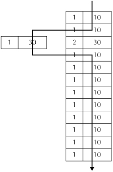
FIGURE 2-1. MVRC at work
A millisecond after this, another user updates a later row, increasing the value from 10 to 20. This change is committed before the query gets to the row, meaning that the newly committed value is included in the query. Although this action is correct, keep in mind that this change means that the final sum for the query will be 150, which is not correct. In fact, the sum of 150 was never correct. When the query began, the correct sum would have been 140. After the row is deleted, the correct sum would have been 110. After the subsequent update, the correct value would have been 120. But the sum would never have been 150. The integrity of the data has been lost. In a busy database with long-running queries, this could happen frequently. If you have a busy database (and who doesn’t), you could be getting a wide variety of incorrect data in your query—not a desirable outcome, to say the least.
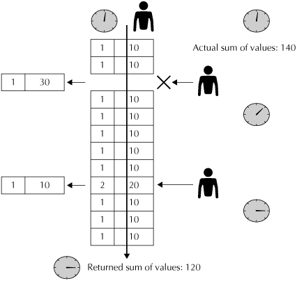
FIGURE 2-2. Summaries without MVRC
Figure 2-3 shows that MVRC handles this scenario correctly. When a query begins, it is assigned a system change number, or SCN. If the query encounters a row with a larger SCN, the query understands that the row has been changed since the query began, so Oracle uses an earlier version of the row to deliver a consistent view of data at a particular point in time. Oracle always delivers a consistent snapshot view of data, all without the overhead of read locks, lock management, and the contention they can cause.
To sum up, with MVRC, readers don’t block writers, writers don’t block readers, and queries always deliver a consistent view of data. Other major database vendors cannot deliver these benefits seamlessly, giving Oracle a significant advantage for the past two decades.
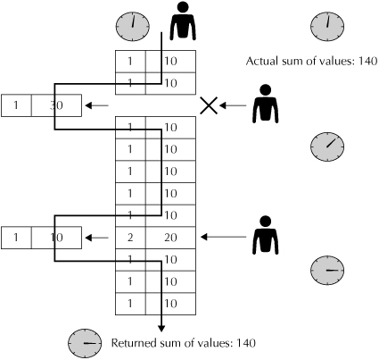
FIGURE 2-3. A consistent view of data with MVRC
Flashback
Before leaving this discussion of MVRC, you should understand that Oracle has leveraged the internal processes and structures used to implement MVRC to add a set of flashback features to the database. As the name implies, flashback is the ability to deliver a view of the database at an earlier point in time. A number of flashback features are available in Oracle 11g:
![]() Flashback query allows users to run queries as if they had taken place in the past with the use of a couple of keywords in a standard SQL statement.
Flashback query allows users to run queries as if they had taken place in the past with the use of a couple of keywords in a standard SQL statement.
![]() Flashback database gives administrators the ability to roll back an entire database to an earlier point in time.
Flashback database gives administrators the ability to roll back an entire database to an earlier point in time.
![]() Flashback drop gives you the ability to remove the effects of one of those unfortunate “oops” moments, when you mistakenly drop a database object.
Flashback drop gives you the ability to remove the effects of one of those unfortunate “oops” moments, when you mistakenly drop a database object.
In addition, many other varieties of flashback are used for different types of operations, including error diagnosis and corrections. Although flashback might just be along for the ride, provided by the infrastructure that supports MVRC, the flashback features can prove to be extremely useful.
Flashback also points out one of Oracle’s great strengths. Since MVRC has been a part of the Oracle database for so long, the supporting technology is robust enough to provide additional functionality with little additional development effort, extending Oracle’s feature advantages.
Real Application Clusters
As mentioned earlier, Exadata technology cannot be seen as springing fully formed from the brow of Oracle. Exadata technology is built on Oracle features that have been shaping the capabilities and direction of the database for many years. The best example of this progression is how Real Application Clusters, almost always referred to by the less unwieldy acronym of RAC, provides the basis for the eventual hardware/software synergies in the Exadata Database Machine.
RAC is the foundation of the Oracle grid story, both figuratively and literally. RAC gave users the ability to create a powerful database server by grouping together multiple physical servers. This capability provides an unmatched value proposition for database servers. That value proposition, and how it is implemented, is explored in the following pages.
What Is RAC?
RAC was the marquis feature of the Oracle 9i release, so most readers will probably be familiar with the general capabilities of this feature. But since RAC and grid are really the first big steps towards Exadata and the Exadata Database Machine, it’s worthwhile to spend a few paragraphs reviewing the exact definition and architecture of RAC.
The official name of the feature does make sense. When introduced, the defining characteristic of RAC was that it could be used transparently with existing, or real, applications. There was no need to rewrite or refactor existing applications to take advantage of the benefits of RAC, a virtue that is common to most new Oracle features.
The second part of the name points to what made RAC different. Normally, an Oracle database is only associated with a single instance—a single running copy of the Oracle database software—which was in turn associated with a single physical server. An Oracle database with RAC could run across multiple instances and servers, as shown in Figure 2-4.
FIGURE 2-4. Architecture of Real Application Clusters
You can see multiple servers, or nodes, which work together through the means of a layer of software called clusterware. Clusterware acts to coordinate the operation of the member nodes as well as to monitor and maintain the health of these nodes. Oracle has its own clusterware, which is bundled with Oracle Database Enterprise Edition.
You can also see that each node has an instance running and that all instances access the same shared storage. This shared storage and the software portion of RAC means that a user can connect to any of the nodes in the cluster and access the same database transparently. The resources of all the nodes in the cluster are combined into a single pool of resources.
The architecture of RAC introduced significant benefits in two key areas—availability and scalability.
RAC and Availability
A single RAC database can include instances on more than one node, which has dramatic implications for the overall availability of an Oracle RAC database. If any single node goes down, the failure has virtually no impact on any of the other nodes, which continue to operate as normal. This continuous operation means that even if a server node fails, the database continues running and does not have to be recovered. And every node acts as this type of hot backup for every other node, so the more nodes added to the cluster, the more reliable the cluster becomes.
To be absolutely accurate, the loss of a server node will affect some RAC users—those who are attached to that node. Just as with a single instance, these users will lose their connection to the database and all in-flight transactions will be rolled back. Users of the failed node will normally have to reconnect to another node, although another Oracle feature, Transparent Application Failover (TAF), can automate this process. The Oracle software stack also offers Fast Application Notification, which sends messages when an instance is not available, and Fast Connection Failover, which automatically reacts to these messages.
In addition, RAC includes distributed resources to manage tracking of data blocks across nodes, which we describe in the section on Cache Fusion later. If a node becomes unavailable, there is a brief pause for all users as the portion of the distributed management database is reassigned to existing nodes, but this pause is typically only a few seconds.
These particulars are minor, but the overall availability advantages are significant—an Oracle instance can disappear without requiring the shared database to be recovered, providing hot standby capability across all the nodes of a RAC cluster.
RAC and Scalability
RAC provides more than just hot standby for an Oracle database. As mentioned previously, a RAC database is completely transparent to the user and their application. This transparency means that administrators can add nodes to a RAC cluster without any changes to applications or user configurations.
This simple statement has fairly profound implications. Assume that you are running out of horsepower with a non-RAC Oracle database. At this point, you will need to acquire a bigger server that you will migrate your database to. This will require administration effort, some downtime, and a fairly large expenditure.
Compare that with RAC. If you have a two-node cluster, you can simply add another server to the cluster to increase the horsepower of the overall database by about 50 percent—without even bringing down the overall database.
RAC does offer linear scalability, in that adding a node to a two-node cluster will increase the horsepower by about 50 percent, or adding a node to a three-node cluster will add 33 percent to the overall power of the cluster. Don’t mistake this type of linear scalability for perfect scalability, in that a two-node cluster will not produce 200 percent of the throughput of a single-node server. However, you will not find decreasing efficiency as you add more nodes to the cluster, crucial to the use of larger clusters.
The scalability of RAC has significant implications for your database budget. With a single database server, you would typically size the server to handle not only today’s demands; instead, you will size the server to handle the anticipated load a couple of years in the future to avoid the overhead of a server upgrade too soon. This approach means that you will end up buying more servers than you need, increasing cost and forcing excess server capacity in the initial stages.
With RAC, you can simply buy the number of nodes you need to handle your near-term requirements. When you need more power, you just buy more servers and add them to the cluster. Even better, you can buy smaller commodity servers, which are significantly less expensive than larger machines. And to top it all off, the server you buy in nine months will give you more power for your money than a similar server today.
All of these benefits are part of the common Oracle liturgy, but there is one other advantage that RAC scalability provides. Even experienced administrators are frequently wrong when they try to estimate the requirements for a database server two years out. If they overestimate future needs, their organizations end up buying excess hardware and software—the lesser of two evils. If they underestimate, they will find themselves having to upgrade their database server early, because the database services it provides are more popular than they expected. So the upgrade, with its concomitant overhead and downtime, affects a popular service.
With RAC, you are never wrong. You won’t overestimate, since you will plan on buying more servers when you need them, whether that is in nine months or five years. And you won’t be plagued by the penalties associated with underestimation.
Cache Fusion
Up to this point, we have been looking at RAC from a fairly high level. You could be forgiven for not appreciating the sophistication of RAC technology. The really interesting part comes when you understand that the instances spread across multiple nodes are not just sharing data—they are also sharing their data caches, which is the key to the performance offered by RAC.
The diagram shown in Figure 2-5 is a slight expansion of the architecture shown in Figure 2-4. The difference is that you can now see the shared cache, implemented by technology known as Cache Fusion.
Although all instances share the same database files, each instance in a RAC database, since it is located on physically separate servers, must have its own separate memory cache. Normally, this separation could lead to all kinds of inefficiencies, as data blocks were cached in the data buffers of multiple machines. Part of the RAC architecture is an interconnect, which links caches on separate servers together and allows transfers directly between different memory caches. This architecture allows the database cache to grow as more nodes are added to a cluster.
When a SQL operation looks for a data block, the instance looks first in its own database buffers. If the block is not found in those buffers, the instance asks the cluster management service if the block exists in the buffer of another instance. If that block does exist in another instance, the block is transferred directly over the interconnect to the buffers of the requesting node.
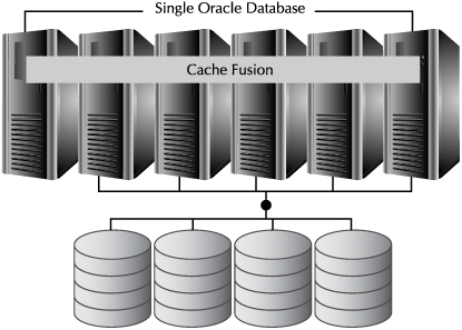
FIGURE 2-5. RAC and Cache Fusion
Cache Fusion uses a global service, where the location of every data block in every cached is tracked. The tracking is spread over all the nodes; this tracking information is what has to be rebuilt in the event of a node failure. RAC uses some intelligence in assigning ownership of a particular block. If the block is usually used on a particular instance, that instance is given the responsibility of tracking that block, cutting down on the interconnect traffic and the transfer of blocks between nodes, reducing any potential bottlenecks caused by flooding of the interconnect.
There may be times when you want to limit the way that a particular application or instance uses the resources of the entire cluster, and RAC provides a number of options, which are described in the next section.
Cache Fusion and Isolation
Did you notice something that was not mentioned in the discussion of Cache Fusion? In the first section in this chapter, you read that the smallest unit of standard data movement is the data block and that a data block can (and usually does) contain more than one row. So what happens if one row in a block is being modified by a transaction on one instance and another instance wants to modify a different row in the same block? Good question, and one that Oracle, unsurprisingly, has covered.
A single row in a data block can be part of an active write transaction and have an exclusive lock on that row. If the block containing that row is requested for a write operation on another row in the block, the block is sent to the requesting node, as expected. However, the node that originates the transfer makes a copy of the block, called a past image, which can be used for instance recovery in the event of a failure or to construct a consistent image of the row, part of the overall operations used to implement multiversion read consistency. When the row is committed on the requesting node, the block is marked as dirty and eventually written to the database. Once this version of the block is safely part of the database, the past image is no longer needed. Metalink (MOS) note 139436.1 explains how instances interact in different locking scenarios in greater detail, if you are interested.
Allocating Resources and RAC
Up to this point in the discussion of RAC, we have been looking at the architecture of RAC as if the cluster were supporting a single database. In fact, RAC is frequently used as a consolidation platform, supporting many databases and instances.
Once you start supporting multiple databases on a RAC architecture, you may find that you want to allocate the computing resources to appropriately serve the different uses of the database—or even modify those allocations, depending on a variety of factors. This section will describe some of the RAC-centric ways to accomplish this task.
Load Balancing, Part One
To a connecting session, a RAC database appears as a single, monolithic database. This key feature is what allows existing applications to take advantage of RAC without modification. But the underlying implementation of RAC involves physically separate servers, and each session will be connected to only one of those servers. How does RAC decide which instance to assign to an incoming connection request?
When RAC was introduced with Oracle 9i, the software determined the connection target by the CPU utilization of the different member instances. A new connection was assigned to the instance running on the server with the lowest level of CPU utilization.
This type of connection assignment did provide more efficient usage of the overall RAC cluster than a random allocation, but the end result was balancing the load for the overall cluster. The process assumed that the entire RAC database was being used equally by all instances. As larger clusters went into production, and as users started implementing RAC to consolidate multiple databases on a single cluster, this single-minded approach was not flexible enough to allocate computing resources appropriately. Enter services.
Services
Services, introduced with Oracle Database 10g Release 2, are a way to provision nodes in a RAC database for specific applications, as shown in Figure 2-6.
You can define which instances handle requests from a service. In this way, you can segregate the processing power provided by an instance to one or more services, as you can assign more than one service to a particular instance.
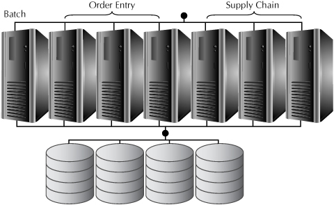
FIGURE 2-6. Services and RAC
You can dynamically adjust which instances handle which services, either in response to external conditions, such as time of day, or to designate which nodes should take on a service in the event of a failure of a node designated for that service.
The configuration of services and nodes is done as part of the RAC configuration, and clients simply connect to a service, rather than the RAC database or an individual node.
Load Balancing, Part Two
Once you define services, you can use a more sophisticated method of allocating resources between different nodes associated with a service.
You can still use the traditional method of allocating connections based on CPU utilization for the service, the same approach that has been used for RAC since its introduction.
You can also assign connections based on more advanced metrics of runtime performance delivered through the means of a Load Balancing Advisory. These advisories are sent to the listeners for each instance involved in a service.
When you use the Load Balancing Advisory, you configure whether you want to determine the connection load balancing based on throughput for an instance or the service time, representing the speed of response, for an instance. The Load Balancing Advisories deliver the information required to determine the appropriate connection assignment based on real-time workload conditions. The dynamic nature of this approach helps to ensure a more balanced workload across service instances, resulting in better utilization of resources automatically.
Load Balancing Advisories can also be delivered to clients so that environments that support client-side connection pooling can benefit from this type of intelligent connection allocation.
Server Pools
The concept of services gives you the ability to assign operations to a specific set of nodes within a RAC database. With Oracle Database 11g Release 2 came the introduction of server pools and quality of service measurements, which take this concept even further.
Services used to be assigned to specific nodes, which was a good way to divide up resources, but this approach required services to be explicitly assigned to one or more instances, which could create an increasing management overhead as the number of configuration options multiplied. A server pool is a collection of nodes, and services are assigned to a pool rather than a set of specific nodes.
RAC uses server pools to allocate resources between different services assigned to a pool. You can define a quality of service policy, described in more detail in Chapter 8, which specifies the performance objectives for an individual service, as well as the priority of that service. If a high-priority service is not getting sufficient CPU to deliver the defined quality of service, RAC makes a recommendation to promote the scheduling priority for that service with the CPU scheduler.
This remedy will improve the performance of the promoted service, which very well may not affect the qualities for the other services in the pool. If multiple services for a pool are all failing to meet their quality-of-service goals, the server pool can implement a different scenario to share resources, using Database Resource Manager (described later) or grab a node from another pool to remedy the problem, although the transfer of this node may take some time, depending on the specific implementation scenario.
The RAC database also uses feedback on the amount of memory used for a single server node in a server pool. If there is too much work for the memory on the node, that node will temporarily stop accepting new connections until the demand for memory is decreased.
Additional Provisioning Options
The Oracle Database includes other ways to provision database server resources, such as Database Resource Manager, which is described later in this chapter, and instance caging, implemented through Database Resource Manager, which allows you to specify how to allocate CPU resources between different database instances that may be sharing a single physical server.
RAC One
A RAC database gives you the ability to take a pool of resources and use them as if they were a single machine. In today’s computing environment, virtualization provides a different approach—the ability to share a pool of resources offered by a single physical machine among multiple virtual machines.
RAC One is a flavor of RAC that delivers the same type of benefit. An instance using RAC One runs on a single node. If that node should fail, the RAC One instance fails over to another node. Since the RAC One database was only running on a single instance, the underlying database will still need to be recovered, but the RAC One software handles this recovery, as well as the failover to another node, transparently, reducing downtime by eliminating the need for administrator intervention.
You can think of RAC One as a way to implement virtual database nodes rather than virtual machines. The purpose-driven nature of RAC One makes administration easier, and the elimination of a layer of virtual machine software should deliver better performance with the same hardware.
RAC and the Exadata Database Machine
Although RAC was introduced before the advent of the Exadata Database Machine, and although there is no absolute requirement that you use RAC on the Machine, the two offerings are made for each other. In fact, the Database Machine is sometimes referred to as a “grid in a box,” and RAC is the foundation of that grid.
The Exadata Database Machine includes a number of physical database servers in the same cabinet, so using RAC to pool the resources of those servers is a natural complement. The Database Machine is also configured for optimal RAC performance as it provides a high-bandwidth interconnect between the database servers.
In addition, since the Exadata Database Machine can be used as a platform for consolidation, there may be scenarios when RAC One is appropriate for this environment.
Automatic Storage Management
Real Application Clusters was a big step forward for the Oracle database. With RAC, you could combine multiple physical database servers together to act like a single database, offering a new way to deploy and scale database servers.
Automatic Storage Management, or ASM, extends a similar capability for storage. ASM was introduced with Oracle Database 10g, and provides a way to combine multiple disks into larger logical units, reducing storage costs and simplifying management. In addition, like RAC, ASM delivers additional benefits, such as improving performance and availability and simplifying a number of key management tasks.
What Is ASM?
ASM is storage management software, providing a single solution for a cluster file system and volume management. ASM manages a collection of storage disks, simplifying the interface to those disks for database administrators. ASM eliminates the need for third-party software like volume managers and file systems for Oracle database environments.
ASM runs as an instance, just like an Oracle database, and the ASM instance has some of the same organization as a database instance. Each database server that will use ASM must have a single ASM instance, which can manage storage for one or more database instances on the node.
The ASM instance maintains metadata about storage. The ASM instance uses this information to create an extent map that is passed to the database instance, which removes the necessity of the database instance to go through the ASM instance for access. The database instance interacts with ASM when files are created or modified, or when the storage configuration is modified by adding or dropping disks. This implementation gives ASM the flexibility to dynamically expand and contract storage, to implement mirroring and striping transparently, without affecting performance.
With ASM, you first build grid disks out of cell disks, which are built on top of LUNs, or logical units, as shown in Figure 2-7.
All management of storage is done at the level of disk groups by the ASM instance. An individual database file must be stored within a single disk group, but a single disk group can contain files from many different database instances. ASM provides a file system interface to the files stored in each disk group.
ASM is included with all editions of the Oracle Database that support Real Application Clusters, which includes Standard and Enterprise Editions. ASM comes with the Oracle database rather than with the RAC option, so you can use ASM for single-instance databases as well as Real Application Cluster databases, providing many of the same benefits for the single instance.
NOTE
ASM relies on Oracle Clusterware to manage multiple nodes in a cluster and synchronization between database instances and ASM, so ASM always requires Oracle Clusterware.
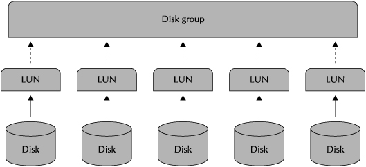
FIGURE 2-7. Automatic Storage Management
ASM and Performance
ASM automatically stripes files across multiple physical disks, which increases the access performance by spreading I/O over multiple disk heads. This placement avoids excessive hot spots in disk files, and also contributes to better I/O performance. ASM normally creates stripes based on the size of the allocation unit (AU) assigned to a disk group, but for some files, such as redo logs, ASM stripes are smaller to reduce I/O latency on these crucial files.
The I/O performance produced by ASM is roughly equivalent to the performance of a raw partition, without having the more extensive management overhead of raw storage.
In some cases, such as a stretch cluster, where nodes of a cluster are widely separated, ASM can give better performance by reading from a more local mirrored copy of data, rather than trying to access the primary copy at a more distant location. This capability is configured by means of an initialization parameter.
Oracle Database 11g Release 2 introduced a new performance feature for ASM called Intelligent Data Placement. A disk is circular, which means that the outer tracks of the disk are moving faster than the inner tracks, resulting in faster read times for data on the outer tracks. You can specify that data for a file or an entire disk group is either on the outside or inside of the disk, providing better performance for the outer sections. This Intelligent Data Placement works well with two disk groups, one for data and one for the Fast Recovery Area (FRA), which is used for backups. The FRA can go on the inner tracks of the disk, ceding the better-performing sections to the data disk groups that are in active production use.
ASM and Availability
In terms of disk storage, ASM provides an availability solution by automatically mirroring data in a disk group. Mirroring data means making an extra copy of the data in the event of a block or disk failure, similar to the functionality provided by redundant arrays of inexpensive disks (RAID) disks. You can choose to mirror data once, to assure reliability if a single point of failure occurs, or twice, to assure reliability even if a second failure should occur. You also have the option of not mirroring data, which you might choose if you are using ASM with a RAID disk that already provided mirroring, although ASM mirroring is specifically designed to support database access. You can assign mirroring on the basis of individual files to implement different levels of redundancy for different scenarios.
You want to make sure that the mirrored image of the data is kept separate from the primary copy of the data so that a failure of the disk that holds that primary copy will not also affect the mirrored copy. To implement this protection, ASM uses the concept of a failure group. When you define a disk group, you also define a failure group in relation to that disk group. Mirrored data is always placed in a different failure group, which ensures that a mirrored copy of the data is separated from the primary copy of that data. If a block fails or is corrupted, ASM will automatically use a mirrored copy of the data without any interruption in service. You can direct ASM to actually repair bad blocks from either a command-line interface or Enterprise Manager.
Normally, a read request will use the primary copy of the data. If the read request for that primary copy fails, ASM will automatically read the data from a mirrored copy. When a read fails in this way, ASM will also create a new copy of the data, using the mirrored data as the source. This approach is automatically used whenever a read request for data is executed and a bad data block is discovered. You can force this type of remapping on data that has not been read by means of an ASM command.
Frequently, disk failures are short-lived, or transient. During a transient disk failure, changes can be made to the secondary copy of the data. ASM keeps track of these changes, and when the disk comes back online, performs an automatic resynchronization to make the now-available copy of the data the same as the copy of the data that was continually accessible. This tracking means the resynchronization process is fast.
ASM and Management
There has always been overhead associated with managing storage for an Oracle database, such as determining which blocks have free space. ASM takes care of all of these issues, removing them from the DBA workload.
In fact, ASM manages much more than these basic tasks. The striping and mirroring discussed in the previous sections is done automatically within a disk group.
You can also dynamically resize a disk group by adding more disks to the group, or take disks out of a disk group. Both of these operations can be performed without any downtime. If you add new disks to a disk group, ASM will rebalance data across the new disks. ASM does an intelligent rebalance, only moving the amount of data necessary to ensure an even balance across the new set of disks, and rebalancing is done, by default, asynchronously, so as to not impact online performance. ASM includes a parameter that gives you the ability to control the speed of rebalancing, which, in turn, has an impact on the overhead used by the operation.
Since ASM manages most administrative details within a disk group, you would normally create a small number of disk groups. In fact, Oracle recommends creating only two disk groups—one for data and the other for the Flash Recovery Area used to hold database backups.
ASM itself can be managed through SQL*Plus, Enterprise Manager, or a command-line interface.
Partitioning
Computing hardware is, in the broadest sense, made up of three basic components—a computing component (CPU), memory, and storage. Over the course of the history of computing systems, different components have been the primary culprits in the creation of bottlenecks caused by insufficient resources. For the last ten years, the main source of performance bottlenecks has been the storage systems that service I/O requests.
To address this area, the Oracle database has continually implemented strategies to reduce the overall demand for I/O operations, such as indexes and multiblock reads for table scans. Partitioning is another of these strategies.
NOTE
As you will see in the next chapter, the Exadata Storage Server takes this approach of reducing I/O to a whole other level.
What Is Partitioning?
A partition is simply a smaller segment of a database object. When you partition an object, you break it into smaller pieces, based on the value of a partition key, which consists of one or more columns.
All SQL statements interact with the partitioned object as a single unified entity, but the Oracle optimizer is aware that an object is partitioned and how it is partitioned. The optimizer uses this information to implement a strategy of partition pruning. A query that needs to implement some type of selection, either with a predicate or a join, can simply avoid reading partitions whose partition key indicates that none of the data in the partition will pass the criteria. In this way, the execution path can avoid accessing a large portion of an object, reducing the overall I/O requirements. The performance gain, like the partition, is implemented transparently.
You can partition both tables and indexes with any of the partition methods that are described in the next section. Three different relationships are possible between a partitioned table and an index, as shown in Figure 2-8.
![]() The index and the partition can be partitioned on the same partition key. This relationship, known as equipartitioning or a local index, means a separate portion of the index for each partition in the database. If most of the queries running against your partitioned table will result in partition pruning, equipartitioning amplifies the benefits of this approach.
The index and the partition can be partitioned on the same partition key. This relationship, known as equipartitioning or a local index, means a separate portion of the index for each partition in the database. If most of the queries running against your partitioned table will result in partition pruning, equipartitioning amplifies the benefits of this approach.
![]() An index could be global and partitioned on a different partition key than the associated table. This scheme will deliver benefits for some queries where the index partition key can be used for partition pruning, and other benefits for queries where the table partition key can be used.
An index could be global and partitioned on a different partition key than the associated table. This scheme will deliver benefits for some queries where the index partition key can be used for partition pruning, and other benefits for queries where the table partition key can be used.
![]() An index can also be global and unpartitioned, and the table is partitioned. Although this relationship may not produce as large a benefit as equipartitioning, some types of random access will work better this way, as a global index can be accessed with a single read rather than having to probe each index partition.
An index can also be global and unpartitioned, and the table is partitioned. Although this relationship may not produce as large a benefit as equipartitioning, some types of random access will work better this way, as a global index can be accessed with a single read rather than having to probe each index partition.
Partitioning Types
Partitioning provides benefits by dividing up a larger table into smaller portions, based on the value of the partition key. A table or index can only be partitioned once at the top level, of course, since partitioning dictates the logical storage of the object, but the partitioning scheme used must correspond with the way that a query will be requesting data in order to provide performance benefits. Because of this, Oracle has continually expanded the ways that you can partition tables since the introduction of this feature with Oracle 8.
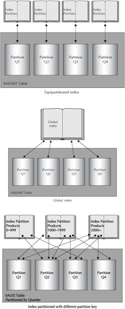
FIGURE 2-8. Index and table partitioning
Oracle Database 11g Release 2, the current release of the database at the time of this writing, supports the following types of partitioning:
![]() Hash The partition key for hash partitions is created by running a hash function on the designated partition column. The hash calculation is used to ensure an even distribution among partitions, even when the distribution of the actual values of the partition column is uneven. A hash-partitioned table cannot use partition pruning when the selection criteria include a range of values.
Hash The partition key for hash partitions is created by running a hash function on the designated partition column. The hash calculation is used to ensure an even distribution among partitions, even when the distribution of the actual values of the partition column is uneven. A hash-partitioned table cannot use partition pruning when the selection criteria include a range of values.
![]() Range Range partitioning uses the actual value of the partition key to create the partitions. Range partitioning is described with a low value and a high value for the partition key, although you can have one partition without a low value for all values lower than the specific value and one partition without a high value for a similar function at the high end. Range partitions can be used for partition pruning with a range of values, either specified or implied through the use of the LIKE operator.
Range Range partitioning uses the actual value of the partition key to create the partitions. Range partitioning is described with a low value and a high value for the partition key, although you can have one partition without a low value for all values lower than the specific value and one partition without a high value for a similar function at the high end. Range partitions can be used for partition pruning with a range of values, either specified or implied through the use of the LIKE operator.
![]() List In a list partition, you assign a specific list of values for a partition key to indicate membership in a partition. The list partition is designed for those situations where a group of values are linked without being consecutive, such as the states or territories in a sales region. List partitions can be used for partition pruning with the LIKE operator.
List In a list partition, you assign a specific list of values for a partition key to indicate membership in a partition. The list partition is designed for those situations where a group of values are linked without being consecutive, such as the states or territories in a sales region. List partitions can be used for partition pruning with the LIKE operator.
![]() Composite Composite partitioning is a way of adding a subpartition to a table, giving the table two levels of partitioning, as shown in Figure 2-9. Composite partitioning allows Oracle to go directly to a partition with specific values in two dimensions. With Oracle Database 11g, you can have any mix of composite partitions that include range, hash, or list partitions.
Composite Composite partitioning is a way of adding a subpartition to a table, giving the table two levels of partitioning, as shown in Figure 2-9. Composite partitioning allows Oracle to go directly to a partition with specific values in two dimensions. With Oracle Database 11g, you can have any mix of composite partitions that include range, hash, or list partitions.
![]() Interval An interval partition is a way to reduce the maintenance overhead for range partitions that use a date or number as the partition key. For an interval partition, you define the interval that specifies the boundaries of a partition. The Oracle Database will subsequently create partitions as appropriate without any further intervention. If the value for a partition key requires a new partition to be created, that operation is performed automatically. You can change an existing range-partitioned table into an interval-partitioned table, as long as the ranges fall into a specific pattern, or you can extend an existing range-partitioned table into an interval table in the future. You can also merge partitions at the low end of an interval-partitioned table to create a single-range partition. This last option is particularly useful for gaining the benefits of an interval partition while implementing an Information Lifecycle Management (ILM) strategy for reduced storage costs.
Interval An interval partition is a way to reduce the maintenance overhead for range partitions that use a date or number as the partition key. For an interval partition, you define the interval that specifies the boundaries of a partition. The Oracle Database will subsequently create partitions as appropriate without any further intervention. If the value for a partition key requires a new partition to be created, that operation is performed automatically. You can change an existing range-partitioned table into an interval-partitioned table, as long as the ranges fall into a specific pattern, or you can extend an existing range-partitioned table into an interval table in the future. You can also merge partitions at the low end of an interval-partitioned table to create a single-range partition. This last option is particularly useful for gaining the benefits of an interval partition while implementing an Information Lifecycle Management (ILM) strategy for reduced storage costs.
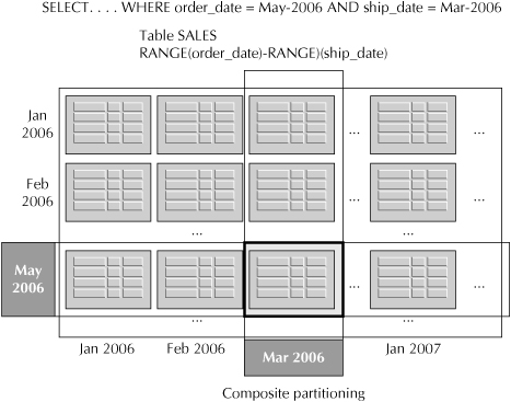
FIGURE 2-9. Composite partitioning
![]() REF A REF partition is another form of partitioning that reduces overhead, as well as saving storage space. Having parent and child tables in a foreign key relationship is a common implementation practice, especially since this architecture allows for partition-wise joins, described in the next section on parallel execution. A REF partition on the child simply points back to the parent and instructs Oracle to use the same partition scheme as the parent, as shown in Figure 2-10. Any changes made in the partitioning scheme in the parent table are automatically implemented in the child table. REF partitioning has an additional benefit with regard to storage. Since both tables are using the same partition key, there is no need to store the key value in the child table, eliminating redundancy and saving storage space.
REF A REF partition is another form of partitioning that reduces overhead, as well as saving storage space. Having parent and child tables in a foreign key relationship is a common implementation practice, especially since this architecture allows for partition-wise joins, described in the next section on parallel execution. A REF partition on the child simply points back to the parent and instructs Oracle to use the same partition scheme as the parent, as shown in Figure 2-10. Any changes made in the partitioning scheme in the parent table are automatically implemented in the child table. REF partitioning has an additional benefit with regard to storage. Since both tables are using the same partition key, there is no need to store the key value in the child table, eliminating redundancy and saving storage space.
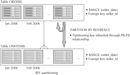
FIGURE 2-10. REF partitioning
![]() Virtual Virtual partitioning allows you to partition a table on a virtual column. The virtual column is defined as the result of a function on existing columns in the table. The virtual column is treated as a “real” column in all respects, including the collection of statistics, but does not require any storage space.
Virtual Virtual partitioning allows you to partition a table on a virtual column. The virtual column is defined as the result of a function on existing columns in the table. The virtual column is treated as a “real” column in all respects, including the collection of statistics, but does not require any storage space.
Other Benefits
Partitions can produce performance benefits by reducing the I/O needed for query results, but partitioning delivers other benefits as well.
To Oracle, partitions are seen as individual units for maintenance operations. This separation means that a partition can be taken off-line independently of other partitions, that maintenance operations can be performed on individual partitions, and that the failure of an individual partition does not affect the availability of the remainder of the table.
TIP
One exception to this availability advantage occurs if a partition has a global index. The global index will be unusable and will have to be recovered if even one partition becomes unavailable.
The ability of partitions to act as separate units means that you can use partitions to reduce storage costs through an ILM approach, moving less frequently accessed partitions to lower-cost storage platforms.
Partitions come with their own set of maintenance operations, including the ability to drop and add partitions to a table without taking the table offline, as well as the ability to merge partitions together or split a single partition into two.
Partitioning and the Exadata Database Machine
The key performance benefit provided by partitioning is a reduction in the amount of I/O necessary to satisfy a query. This key benefit is dramatically expanded with a number of Exadata features, such as Smart Scan and storage indexes, which are described in the next chapter.
But these features simply amplify the approach of partitioning. All the benefits of partitioning still apply to the use of the Exadata Database Machine. In this way, partitioning is the start of the performance enhancement continuum delivered by the Exadata Database Machine and, as such, is as integral to the overall benefits provided as RAC is for the use of the database servers.
Parallel Execution
Parallel execution, or parallelism, has been a part of the Oracle database for more than a decade. This long-time feature has become even more important in the context of the Exadata Database Machine, where multiple nodes, CPUs, and intelligence in the storage systems can increase the speed of individual parallel tasks as well as handle more of these tasks at the same time.
What Is Parallel Execution?
Normally, SQL statements are executed in a serial fashion. A statement comes to the Oracle database and is assigned to a server process to execute. A database server has many user processes active at any point in time, and each statement was assigned to a single server process.
NOTE
This description applies to a dedicated server, where there is a one-to-one connection between a user request and a user process on the server. Oracle also supports shared servers, where one server process is shared between multiple user requests, but that technology is outside the realm of this chapter.
Parallel execution is a way to reduce the overall response time of a statement by having multiple processes work on the statement together. By dividing the work up among these multiple processes, or parallel servers, each server does less work and finishes that work faster.
As you will read shortly, there is some overhead involved with this distribution of work, as well as with the re-aggregation of the results of the parallel work, but the overall performance benefit of the parallel operations provides benefits for longer-running operations in most cases.
What Can Be Parallelized?
The Oracle Database can parallelize a range of SQL statements. Table 2-1 lists the SQL tasks that can be executed in parallel.
The tasks listed in Table 2-1 are not all SQL statements. The actual implementation of parallelism takes place at the level of the subtasks that make up the overall execution of a statement. As an example, the query listed next has four subtasks that can be run in parallel—a table scan of each of the two tables, the join operation, and the aggregation requested.
SELECT customer_name, sum(order_total) FROM customers, orders WHERE
customers.customer_id = orders.customer_id
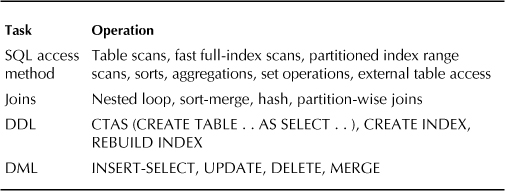
TABLE 2-1. Parallel Tasks
How Parallelism Works
In order for parallelism to be implemented, a database has to divide the data that is the target of a task into smaller groups for each separate parallel process to work on. The Oracle Database uses the concept of granules. Each granule can be assigned to a single parallel process, although a parallel process can work on more than one granule.
NOTE
In fact, parallelism can be more efficient if each parallel process works on more than one granule. When a process finishes its work on a granule, the process can get another granule to work on. This method of distribution avoids the potential problem of the convoy effect, when the completion of the overall task is only as fast as the slowest parallel process. If a parallel process completes its work, rather than sit around waiting for its peers, the process simply begins work on another granule.
With Oracle, a granule can either be a partition or a range of data blocks. The block-based granule gives the Oracle Database more flexibility in implementing parallelism, which can result in more SQL statements and tasks that can benefit from parallel operations.
The Architecture of Parallel Execution
When the Oracle Database receives a SQL statement that can be executed in parallel, and when parallelism is enabled for that instance, the parallel execution process begins, as shown in Figure 2-11.
In first step of parallel processing, the server process running the statement becomes the parallel query coordinator, shown as QC in the diagram. The QC is responsible for distributing and coordinating work among the parallel server processes, shown as PX in the diagram.
The query coordinator communicates with the parallel servers through a pair of buffers and, in most cases, the parallel servers communicate with each other through another set of buffers.
Parallelism at Work
Now that you know the basics of parallelism in Oracle, we can walk through a couple of examples of parallelism in action.
The first example is a simple table scan, as shown in this SQL statement:
SELECT * FROM customers;
The query coordinator divides the target data up into granules and assigns a granule to each parallel server in a set of parallel servers. As a parallel server completes the table scan of a granule, the results are returned to the query coordinator, who combines the accumulated results into a result set to return to the user. That example is simple enough.
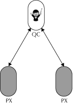
FIGURE 2-11. The architecture of parallel execution
The process gets a little more complicated when there are multiple tasks within a query that can benefit from parallel processing. Let’s return to the SQL statement originally mentioned in the previous section:
SELECT customer_name, sum(order_total) FROM customers, orders WHERE
customers.customer_id = orders.customer_id
The query coordinator will assign granules for scanning one table to one set of parallel servers, the producers. Once the producers complete scanning that table, they send the resulting rows to the second set of parallel servers, the consumers, and begin to scan the second table. Once the consumers start to receive rows from the second table scan, they will begin doing the join. As the producers start to send rows to the consumers, they will have to redistribute the rows to the appropriate consumer process in order to complete the join.
The query coordinator has a number of options for redistributing the data, as shown in Table 2-2.
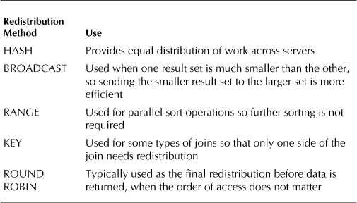
TABLE 2-2. Redistribution Methods
The results of the join are sent to a set of parallel servers for sorting, and finally to a set of parallel servers for the aggregation process.
Although this discussion has mentioned several different sets of parallel servers, any SQL statement can only use two sets of parallel servers at a time. These two sets of servers can act together, as producers and consumers. In this example, the set of parallel servers that was going to perform the sort act as consumers of the results from the parallel servers that were doing the join operation.
Partition-wise Parallel Joins
The reason why the previous pages went into some depth on the mechanics of parallel processing is to allow you to understand one of the great goals of parallel execution: partition-wise parallel joins.
Parallel processing is whizzing around in the Oracle database, with loads of parallel processes working together, completing tasks in a fraction of the time of a single serial process. Allowing parallelization for subtasks is a great way to amplify the overall gains from parallelism, but this method can also add some overhead. In the previous description, you may have noticed one particular type of overhead that could be significant—the redistribution of data in order to perform a join.
There is a way you can completely avoid this overhead through the use of parallelism in coordination with partitioning. Figure 2-12 illustrates the difference between a standard parallelized join operation, which requires redistribution of data, and a partition-wise parallel join.
In order to accomplish a partition-wise parallel join, both tables have to be equipartitioned using the same partitioning method, and both tables have to have an equal number of partitions.
In the join illustrated on the right in Figure 2-12, the two tables that are to be joined are both partitioned on the key value used in the join. The underlying partitions ensure that the results of a table scan from a partition on one table will only ever be joined with the results of the table scan on the matching partition in the other table.
By eliminating the need to redistribute data, a partition-wise parallel join can deliver better response time than queries that require standard joins. The superior performance of the partition-wise parallel join can influence the partitioning schemes you put in place for your overall database, depending on the usage scenarios for your data. In fact, partition-wise parallel joins only need a single set of parallel servers—there is no need for a set of producers and another set of consumers.
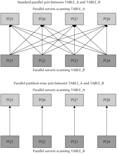
FIGURE 2-12. Standard parallel join and a partition-wise parallel join
How Do You Configure Parallel Execution?
At this point, you understand how the Oracle Database uses parallelism to improve response time. The database does all of this work transparently. But obviously, you have to configure the resources that will be used for implementing parallelism.
Enabling Parallel Execution
Parallel execution is enabled for the Oracle Database by default. However, you can turn parallelism off for a session with the following command:
ALTER SESSION DISABLE PARALLEL (DML | DDL | QUERY);
This command allows you to disable parallel execution for DML, DDL, or query operations. The command can also be used to turn on parallelism for any of these types of operations by replacing the keyword DISABLE with the keyword ENABLE.
NOTE
The ALTER SESSION . . . PARALLEL statement has a third option, FORCE, which you will learn about in the next section.
There are two more places where you can specify the use of parallelism. You can define a particular object with the PARALLEL n clause, which indicates that the object will use parallel execution, with n representing the degree of parallelism (which you will learn more about in the next section). You can also include a PARALLEL hint in your SQL statement.
These three methods are used to allow parallelism for different types of SQL statements. For queries and DDL, you need to have any one of these methods in action—an ALTER SESSION ENABLE command, a PARALLEL clause on an object in the SQL, or a hint in the SQL.
For DML, you will need to have issued the ALTER SESSION command and either have a hint in the SQL statement or have created one of the objects in the statement with a PARALLEL clause.
Enabling Parallel Servers
Enabling parallelism is the first step in its configuration. As you read previously, the query coordinator gets a set of parallel processes, but from where? Oracle uses a pool of parallel processes to serve the needs of parallel execution across the database.
The number of parallel servers you have on an instance has two potential effects. You want to have enough parallel servers to properly service the requests for parallel execution, which delivers the performance increase, but you don’t want to have too many parallel servers, since these servers use resources whether they are in use or not.
There are two initialization parameters you can use to allocate the pool of parallel servers. The PARALLEL_MIN_SERVERS parameter specifies the number of parallel servers to initially allocate when the instance starts up. The PARALLEL_MAX_SERVERS parameter indicates the maximum number of parallel servers to allocate. If your PARALLEL_MIN_SERVERS is less than your PARALLEL_MAX_SERVERS, Oracle will spin up additional parallel servers in response to demand until the maximum number is allocated to the pool.
NOTE
Why so much detail? In the other sections of this chapter, you basically learned about the capabilities of a feature, but not this type of drill down on configuration and the like. The reason for this increased focus on administration is so that you can understand the options you have for implementing parallel execution, options that will become more relevant in the rest of this chapter.
At this point, you know how parallel execution works, how to enable parallelism for an instance, and how to configure a pool of parallel servers. But how does Oracle know how many parallel servers to allocate for any particular statement? The answer lies in the next section.
Degree of Parallelism
You can configure the number of parallel servers to handle all the parallel execution requests for the entire instance, but how do you control how many parallel servers are used for a particular statement? The number of parallel servers used for a statement is called the degree of parallelism for the statement, commonly abbreviated to DOP.
Setting the DOP
You can set the default degree of parallelism at four different levels. First of all, the default DOP for a database is calculated with the following formula:
CPU_COUNT * PARALLEL_THREADS_PER_CPU
The CPU_COUNT parameter is normally set by the Oracle database, which monitors the number of CPUs reported to the operating system, and the PARALLEL_THREADS_PER_CPU also has a default, based on the platform, although the normal default is 2. You can set either of these parameters yourself if this default allows for too many parallel servers, or if the system is I/O bound, which could represent the need to split I/O operations further with parallel execution. Default DOP will be used when the parallel attribute has been set on an object explicitly or via a hint but no parallel degree was specified.
You can also set a specific DOP for an individual table, index, or materialized view, either when you create the object or subsequently modify it. If a SQL statement includes objects with different DOPs, Oracle will take the highest DOP as the DOP for the statement.
The ALTER SESSION command was discussed earlier in this section with regard to enabling parallelism. This command has another format that allows you to specify the degree of parallelism:
ALTER SESSION FORCE PARALLEL (DML | DDL | QUERY) PARALLEL n;
where n is the DOP for the duration of the session.
Finally, you can include a hint in a SQL statement that specifies the DOP for the statement.
A particular SQL statement may have multiple defaults that apply to the statement. The order of precedence for the DOP is hint, session, object, database, so the DOP indicated in a hint will be used instead of any other DOP that is present.
DOP in Action
The last step in understanding how the degree of parallelism affects parallel operations is to understand exactly how this value is used in the runtime environment.
If your Oracle instance has parallelism enabled for a particular type of statement, the optimizer will calculate the degree of parallelism for that statement. A statement can only have a single DOP, which will dictate the number of parallel servers used for all subtasks.
When the statement execution begins, the query coordinator goes to the parallel server pool and grabs the number of parallel servers that will be required for execution—either the DOP or twice the DOP, if the execution will involve both producers and consumers. If no parallel servers are available, the statement will be run serially.
But what if some parallel servers are available in the pool, but just not enough to satisfy the full request? In this case, the query coordinator will take as many parallel servers as it can and adjust the DOP for the statement accordingly—unless the initialization parameter PARALLEL_MIN_PERCENT is set, in which case the statement can fail to execute at all, as explained later in this section.
Modifying DOP
That last statement may have caused you some concern. Here you are, carefully calculating and setting the DOP for objects, sessions, and statements in order to produce the best performance from your Oracle instance. But an instance can support many users, applications, and SQL statements, so you may have a situation where there are not enough parallel servers to go around at a particular point in time. You may not want to populate the parallel server pool with enough servers to guarantee a full DOP during times of peak demand, since this may waste resources most of the time. What will you do?
Oracle has provided several different ways to address this situation dynamically.
One method is adaptive parallelism, enabled by setting the PARALLEL_ADAPTIVE_MULTI_USER parameter. When this parameter is set to TRUE, the Oracle instance will adjust the DOP for statements while taking into account the workload at the time of execution. The goal of adaptive parallelism is to ensure that there will be enough resources available for all parallel executions, so the Oracle instance will reduce the DOP when appropriate.
Adaptive parallelism takes a fairly aggressive approach to ensuring that there are sufficient parallel resources, and this approach may lead to different DOPs being set for the same statement at different times. If you choose to use this approach to limiting parallelism, you should make sure to test its effect on your true runtime environment.
Another method of limiting the DOP is through the use of the Database Resource Manager, which you will learn more about later in this chapter. With Database Resource Manager, you can limit the DOP of all statements, depending on which consumer group is executing the statement. Since membership in consumer groups can change based on runtime conditions, this method gives you the ability to only limit DOP when conditions require it. The DOP specified by Database Resource Manager also takes precedence over any other default DOP, so the limitations of your resource group are always enforced.
Oracle Database 11g Release 2 has an even better solution for addressing this problem, called Automatic Degree of Parallelism, or Auto DOP. Auto DOP does more than just guarantee that a statement will run with a certain DOP—it gives you much more flexibility to control parallelism across the board.
With Auto DOP, Oracle follows the decision process shown in Figure 2-13.
The first step in the process is when the optimizer determines if a particular statement will even benefit from parallel execution by comparing the estimated execution time with the PARALLEL_MIN_TIME_THRESHOLD parameter, set to ten seconds by default.
If the execution time exceeds this threshold, the next step is to calculate the ideal DOP, which is accomplished in the standard way of determining the DOP from different levels of defaults. Once this ideal DOP is calculated, the value is compared with the PARALLEL_DEGREE_LIMIT parameter, which can be used to limit the overall degree of parallelism for the instance, normally set based on the number of CPUs in the system and the parallel threads allowed per CPU. The default value for PARALLEL_DEGREE_LIMIT is default DOP or CPU_COUNT X PARALLEL_THREADS_PER_CPU.
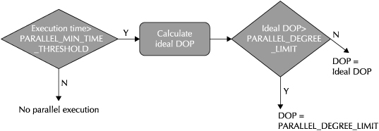
FIGURE 2-13. The Auto DOP decision process
All of these methods will reduce the DOP, depending on environmental conditions. Although this approach prevents your system from slowing down, due to excessive demands for parallelism, it creates another problem. Assuming you assigned a DOP for a reason, such as ensuring that a statement ran with a certain degree of performance, simply toning down the DOP will not give you the desired results. So must you always accept a reduction in performance for the good of the overall environment?
Ensuring DOP
Reducing the DOP for a statement can be more than an inconvenience. Take the example of creating a table and loading data, which is done on a nightly basis. The statement has a DOP of 16, uses both producers and consumers, and completes in three hours with this degree of parallelism in our example. When the statement goes to execute, the parallel server pool only has eight parallel servers available. The statement grabs them all, but ends up with a DOP of 4, due to the need for two sets of parallel servers. Oops—the job now takes 12 hours, and runs over into your production window, which interferes with business operations.
This outcome is especially annoying when you consider that the number of available parallel servers is constantly changing and that the scarcity of parallel servers may have been a transitory phenomenon, with a full complement of parallel servers becoming available seconds or minutes later.
There are two features in Oracle Database 11g that can protect you from this outcome. The first method, which is not new to Oracle Database 11g, is blunt, but effective. The PARALLEL_MIN_PERCENT parameter dictates the minimum percentage of parallel servers that must be available for a statement to execute. With the previous example, you could set the PARALLEL_MIN_PERCENT for the session to 50, which translates to 50 percent. This setting would require the assigned DOP to be at least 50 percent of the default DOP. In the previous example, the statement would actually return an error. You would have to handle this error in your script or code, but at least you would avoid a scenario when a simple lack of parallel server processes affected your production environment. A little bit more code, and a slight tolerance for slower execution, in return for protecting your overall production environment.
Once again, Oracle Database 11g Release 2 has a better solution in the form of parallel statement queuing. As its name implies, statement queuing puts statements into an execution queue when they need a degree of parallelism that cannot be satisfied from the currently available pool of parallel servers. The decision tree process for statement queuing is shown in Figure 2-14.
Once a statement is put into the parallel statement queue, it remains there until enough parallel server processes are available to run the statement with the proper DOP. The queue uses a first-in, first-out scheduler, so parallel statements will not be delayed by other statements with a smaller DOP placed in the queue later.
If you do not want a statement placed into this queue, you can use a hint on the statement itself.
Statement queuing will only kick in when the number of parallel servers in use is greater than a number you specify—a value less than the total number of parallel servers, but one that prevents this process from proceeding in environments where this type of alternative is not necessary. You can also force a statement to be queued, even if the parallel server limit has not yet been reached, with a hint in the statement.
Please keep in mind that the best solution for implementing the proper DOP is always to do a thorough analysis of your parallel execution needs and your environment and set the DOP appropriately. Even the Auto DOP feature will not ultimately deliver the same benefits produced from this measure of planning and foresight.
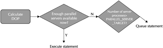
FIGURE 2-14. Decision tree for statement queuing
Parallelism and RAC
In a RAC database, parallel server pools act as a shared resource for all nodes. If there are 64 parallel servers on each node in a four-node cluster, the RAC database sees an overall pool of 256 parallel server processes. This abundance is, in many ways, a good thing, but with some potential downside.
As the previous explanations showed, quite a bit of communication can take place during the parallel execution of a statement, both between the query coordinator and different parallel processes. This communication can have an impact in a RAC environment.
Suppose you had parallel servers spread over all the different nodes and these servers had to redistribute the results of a subtask. Internode communication takes place over the interconnect between nodes, and a flood of traffic could affect the performance of this crucial resource.
NOTE
The Database Machine uses InfiniBand as the interconnect, which can normally handle this type of traffic.
Oracle Database 11g uses an intelligent default approach to distributing parallel server processes. When the database goes to execute a statement in parallel, Oracle will first try to run the statement with parallel servers on the node that is executing the statement. If this cannot be done, the RAC database will look for another node that can supply enough parallel server processes to execute the statement with the calculated DOP. When these two options are not available, parallel servers from multiple nodes will be used.
CAUTION
There is one caveat to this default approach. If the DOP used is the default DOP for the database, RAC will simply grab processes from across all nodes—yet another reason to spend some time analyzing the usage patterns for parallel execution and setting DOP defaults more specifically.
In addition to this default approach, you can specifically limit the allocation of parallel servers to one or more nodes. By setting the PARALLEL_FORCE_LOCAL parameter to true, you only allow the use of parallel processes on the node where the statement is executing. You can also define instance groups, a collection of nodes, and limit the use of parallel servers to the nodes in a particular instance group.
In-memory Parallel Execution
In-memory parallel execution is another new feature introduced in Oracle Database 11g Release 2. This enhancement is another way that Oracle combines the benefits of parallel execution with a RAC environment.
When a RAC database executes a statement with parallel processes, the database checks to see if the objects referenced by the statement could be cached in the aggregated data buffers across all nodes in the server. (This decision is based on a set of heuristics, rather than a simple size calculation.) If there is enough cache available, the granules created for parallel execution are stored in memory on separate nodes, and all operations on those granules are executed on those nodes. This arrangement delivers the benefits of caching entire objects in memory without needing to have the entire amount of memory on a single node.
The data remains cached on the specific node, so if subsequent SQL statements run with parallel execution require this data, the request is sent to the node and the end results returned to the requesting node.
Parallelism and Exadata
Parallel execution, like RAC and partitioning, is designed to work very well in a grid environment. Since the Exadata Database Machine is engineered to be a tightly connected grid, parallelism is ideal for producing great results on this platform. But the Exadata Storage Server provides even more parallelism.
Exadata Storage Servers, which will be covered in detail in Chapter 5, consist of an array of storage systems, and these systems use parallel operations to speed performance.
This storage parallelism does not in any way negate the power of parallel execution for SQL statements. Rather, the parallelism in storage acts as an I/O speed-up for all SQL statements, even for statements that execute serially on database server nodes. The end result is that you may not see as large a difference between serial execution of a statement and the parallel execution of the same statement, but the parallel execution will still provide a significant performance improvement.
Data Guard
A significant part of the overall Exadata Database Machine value proposition is the high availability provided by redundancy throughout the box. Data Guard is a way to supplement this high availability with a disaster recovery solution to provide protection against all types of failures.
What Is Data Guard?
High availability is a quality that, at its core, refers to the absence of a condition. A highly available solution is one where there is little or no downtime.
Traditionally, high availability has been implemented through redundant components in hardware and supporting software capabilities. Real Application Clusters, for instance, allows for the use of multiple servers, with each server acting as a hot failover for the others, without requiring any application changes to take advantage of this feature.
But there are scenarios where even this type of redundancy is not sufficient to avoid downtime, scenarios where a failure affects all the components of a redundant solution, such as a broad power failure or structural issue in an entire building, neighborhood, or region. These occurrences are appropriately referred to as disasters.
Data Guard is used to protect against these disasters by means of a standby database. The standby database can be virtually any distance from the primary database. Data Guard is used to keep the contents of the standby database in sync with the primary database. If the primary database fails, users can reconnect to the standby database after a brief recovery operation and continue their work.
The scenario described is termed a failover, where the standby database takes over for the primary database after that database fails, usually unexpectedly. Data Guard can also be used for a switchover, where the standby database takes over for the primary database intentionally, for situations such as maintenance work on the primary database that require downtime.
How Can Data Guard Be Implemented?
The basic function of Data Guard is to provide a standby database for failover or switchover. Data Guard implements this functionality by shipping redo log information from the primary database to the standby database. Once the redo arrives at the standby database, the records are applied to that database to synchronize it with changes on the primary database.
Modes of Redo Transmission
Although the redo is used to synchronize changes on the standby database, you have options on how the primary database interacts with this operation. You can specify that the redo stream is written to the standby database synchronously, which means that the transaction is not committed until the redo data is written to both the primary redo log and the standby redo log. This option can result in delays on the primary database, but guarantees that no data will ever be lost in the event of a primary failure.
You can also specify that the redo stream is written asynchronously to the standby database, which means that there is no performance impact on the primary database. However, with this mode, the standby database is usually a little behind in getting redo data, so a failure on the primary database could result in some data loss.
Data Guard also gives you the option of the best of both worlds. Redo data is written synchronously to the standby database as long as the redo transmission stream is not causing any delays. Once delays occur, the primary database switches to asynchronous redo data transmission. If the cause of the delay is transient and redo transmission can again be performed synchronously, Data Guard switches back to that form of operation. Although you cannot guarantee zero data loss with this method, you will get this level of integrity in normal conditions with little or no impact on the performance of the primary instance.
Standby Database Types
You also have three choices for configuring the Data Guard standby database, shown in Figure 2-15.
The implementation shown at the top of the figure is called a physical standby database where the redo data comes to the standby database and is then applied to the physical standby. Since the redo is being directly applied to the standby database, this database must be identical to the primary database. Redo information is normally only applied to a database while the database is in the process of recovery from a failure, so a physical standby database is in an ongoing state of recovery. This state means that the standby database is not available for use.
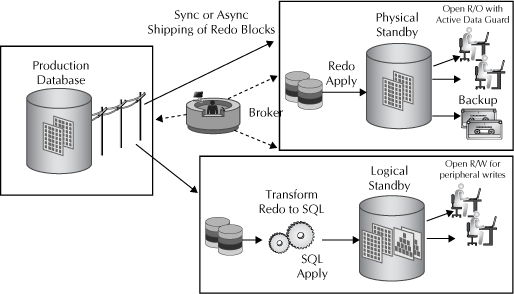
FIGURE 2-15. Data Guard implementations
The implementation shown in the lower half of the figure is called a logical standby database. In this option, the redo data is converted into SQL statements that implement the changes made on the primary database. The SQL statements are then run against the standby database. Since changes are being made through SQL statements, the standby database is available for users. The use of SQL for updates means that there is no need for the standby to be an exact copy of the primary database—the standby can have additional structures, such as indexes, on tables used for standby as well as additional tables that are not on the primary database. Users can access the data in the standby database, and even perform write operations to the tables that are not in the primary database.
Logical standby does have some limitations, including a delay in the application of the redo, since the SQL conversion takes some time, and some limitations on what sorts of changes can be mined from the redo data.
Standard Data Guard, which supports both physical and logical standbys, comes as a part of the Enterprise Edition of the Oracle Database. Oracle also offers an option called Active Data Guard. Active Data Guard works on a physical standby, but allows that standby to be open for read activity even while the redo information is being applied. This capability means that the standby database can be used to offload some of the operations of the primary database, such as reporting or acting as the source of backup operations. Active Data Guard also delivers other benefits, such as detecting bad data blocks on either the primary or standby databases and correcting these blocks with valid copies from the alternative source.
Data Guard also gives you the ability to create a snapshot standby database. A snapshot standby database begins as a physical standby. At a point in time, you discontinue the application of redo information to the standby, allowing the database to be opened for both read and write operations. The redo data continues to stream to the standby, but is not applied. You can change the snapshot standby database back into a physical standby database by applying the accumulated redo data.
Data Guard Broker
Figure 2-15, shown earlier, includes a component that has not been discussed. The Data Guard Broker is a helper application that can be used to automate many of the maintenance operations required for Data Guard, including setting up and managing Data Guard configurations and, more importantly, handling switchover and failover operations with a minimum of operator intervention.
Data Guard and Exadata
As mentioned already, an Oracle database running on the Exadata Database Machine is, in virtually all respects, just a normal Oracle database. This fact means that any application that works against the proper version of a standard Oracle database will work on an Oracle database on the Database Machine with no changes, and that all the standard tools and utilities will work on these Oracle databases.
This statement is also true for Data Guard, with one exception. You will learn in the next section about Exadata Hybrid Columnar Compression. If you used this type of compression, Data Guard will still work properly, sending redo data to the standby database and applying it. However, if the standby target is not an Exadata Database Machine, data that used Exadata Hybrid Columnar Compression will not be available on the standby database. You can still use Data Guard, but to ensure the ability to fail over to the standby, you will have to forego the use of the data that used Exadata Hybrid Columnar Compression, at least until you perform an ALTER statement on the compressed data to decompress it on the standby server.
Compression
The Exadata Database Machine produces fairly dramatic performance improvements for an Oracle database. Part of this improvement comes from improved speed and capacity for all components of the machine, from CPUs to the network to the disk drives. Another part of the improvement comes from reducing the demand for resources, which contributes to improved throughput. Compression, in various options, has been a part of the Oracle Database for more than a decade, and compression can improve overall resource utilization by reducing the size of data, which reduces storage costs and I/O operations, in return for some CPU costs for the compression and decompression operations.
What Types of Compression Does Oracle Support?
Compression was first introduced with Oracle 9i. This initial compression option is known as table compression. With table compression, data was compressed with direct load inserts, which typically are only used with batch operations.
Oracle Database 11g Release 1 introduced a new form of compression referred to as OLTP compression. This new compression differed from table compression in several ways. First of all, Oracle Database 11g can read data in compressed blocks directly, meaning that read operations would not be affected by OLTP compression.
OLTP compression comes as a part of the Advanced Compression option, which also includes a variety of other compression technologies used to compress SecureFiles (large objects), backup sets, and network traffic.
Most importantly, OLTP compression provides compression for data that is inserted after the initial load without affecting write performance. The method used by OLTP compression to accomplish this is shown in Figure 2-16.
Data is compressed within a block on the initial load of data. Data added to a block is initially stored without compression, but when a block contains a sufficient amount of uncompressed data, the block is added to a compression queue, which performs compression as a background process. With this method, data added or changed after an initial load is eventually compressed without affecting the real-time write operation for the data.
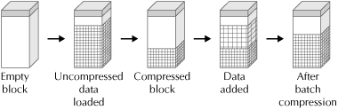
FIGURE 2-16. OLTP compression
SecureFiles
Oracle Database 11g also introduced SecureFiles, which provides compression for large objects stored in the database. SecureFiles gives you the option of three different levels of compression, where the effectiveness of the compression is balanced against the impact on CPU overhead.
Just as compression increases the effectiveness of storage by reducing the space requirements of data, SecureFiles goes an extra step by offering deduplication of large objects. Deduplication computes a hash value for stored large objects so that these objects can be uniquely identified. If an operation attempts to insert another copy of an existing object, SecureFiles simply adds a pointer to the already existing copy of the object. By reducing the number of large objects stored, SecureFiles improves storage efficiency, with no impact on read or write operations.
Benefits of Compression
Of course, compressing data means that you either need less storage for your data or you can store more data in the same storage. In either case, you will save money on storage.
But keep in mind that compressed data means that a compressed data block contains more data, which can mean fewer I/O operations to retrieve a set of rows. In addition, compressed data takes up less space in memory, which means more data blocks in the buffer cache and an improvement in the utilization of this cache. Taken together, these benefits can result in improved performance for some I/O operations, such as table scans, as well as increased overall query performance, based on a higher utilization of data in the buffer cache.
All the benefits delivered by table compression and OLTP compression are also produced by Exadata Hybrid Columnar Compression, which is exclusive to the Exadata platform and which you will learn about in the next chapter.
Remember that all types of compression do require some CPU and memory resources to compress the data when it is added or loaded to the database.
Database Resource Manager
Up to this point, most of the focus of our discussion concerning Oracle Database 11g features has been about providing better performance and scalability through reducing resource requirements. But, fortunately for our job security, there seems to be no end to the increasing requirements for computing services, which means we will all be forced to reckon with the situation where demand is greater than supply.
It is at times like these that we have to remember that performance is really not about resources at all—it’s about expectations. Good performance is the result of user expectations of performance being met. And expectations build on consistency. If the responsiveness of an application varies wildly based on differing specific characteristics of an enterprise-wide workload, you can’t really get away with saying that the performance is good sometimes and even better at other times.
The Database Resource Manager is a tool you can use to ensure consistent performance for critical groups of users and critical tasks to the business. Database Resource Manager not only helps to satisfy users with consistent performance, but also ensures an efficient allocation of oversubscribed resources.
What Is Database Resource Manager?
A database does many things, including manage resources between a group of users. In this way, the database server is responsible for some of the same tasks that an operating system performs. An operating system can allocate resources based on priorities, but the underlying operating system cannot allocate these resources differentially based on individual database users, since these users are not discernable to that software.
Database Resource Manager gives you the ability to prioritize resources to different users. You can specify how computing power is shared among different groups of users and guarantee that some groups will be able to use a fixed percentage of CPU time.
How Does Database Resource Manager Work?
There are three basic components used by Database Resource Manager, as shown in Figure 2-17.
The first component is the consumer group. A consumer group is a collection of sessions. A session is associated with a consumer group when the session is first created, either through mapping rules for sessions, which are defined as part of the resource plan, explained in the next paragraph, or a default consumer group associated with a particular user. Sessions can change resource groups in response to changing conditions, such as demand for resources, but each session can only be a member of a single consumer group at a time. The resources assigned to a consumer group are shared equally with all sessions within the group.
A resource plan is a scheme for sharing the overall resources available to an Oracle instance. The resource plan is made up of directives, which implement the sharing and limitations of resources between consumer groups.
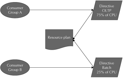
FIGURE 2-17. Components of Database Resource Manager
These three components work together at runtime, where each consumer group is assigned to one or more directives. As shown in Figure 2-17, the OLTP group is guaranteed 75 percent of CPU resources in scenarios where Database Resource Manager directives are in force, while the REPORTING consumer group is guaranteed 25 percent of CPU resources in the same circumstances.
What Can Database Resource Manager Affect?
Resource plans in Database Resource Manager can be used to allocate or limit a number of different resources, including:
![]() CPU usage You can create a directive that limits the percentage of CPU resources for a consumer group. You can have multiple levels of directives, or subplans, for CPU allocation. Each level in a subplan can allocate up to 100 percent of resources, with any remaining resources passed on to the next level for further allocation. You can have up to eight levels of subplans.
CPU usage You can create a directive that limits the percentage of CPU resources for a consumer group. You can have multiple levels of directives, or subplans, for CPU allocation. Each level in a subplan can allocate up to 100 percent of resources, with any remaining resources passed on to the next level for further allocation. You can have up to eight levels of subplans.
![]() Number of active sessions A directive can limit the number of active sessions for a consumer group. If this limit is reached, subsequent session requests are placed into a queue to wait for a currently active session to end. You can designate a timeout period to eliminate sessions that wait in the queue too long.
Number of active sessions A directive can limit the number of active sessions for a consumer group. If this limit is reached, subsequent session requests are placed into a queue to wait for a currently active session to end. You can designate a timeout period to eliminate sessions that wait in the queue too long.
![]() Degree of parallelism You can specify the degree of parallelism (DOP) for a consumer group. At runtime, this DOP is compared with the DOP calculated for an operation, and the lower of the two numbers is used.
Degree of parallelism You can specify the degree of parallelism (DOP) for a consumer group. At runtime, this DOP is compared with the DOP calculated for an operation, and the lower of the two numbers is used.
![]() Sessions You can specify that a session is to be terminated, based on a number of measures, such as the overall execution time for the session, the amount of idle time the session has used, or the amount of undo used by the consumer group. If the undo limit is reached, the DML statement currently executing is terminated and no other DML is allowed until undo space for the consumer group is freed.
Sessions You can specify that a session is to be terminated, based on a number of measures, such as the overall execution time for the session, the amount of idle time the session has used, or the amount of undo used by the consumer group. If the undo limit is reached, the DML statement currently executing is terminated and no other DML is allowed until undo space for the consumer group is freed.
Other Factors
There are a number of conditions that apply to the runtime operation of a resource plan. The overriding condition is that a resource plan and its associated directives only start to operate when the CPU is 100 percent utilized. If there is enough CPU to satisfy all requests, there is no need to allocate that resource.
NOTE
The latest release of Database Resource Manager includes the ability to set an upper limit for CPU resources, which is enforced whether this resource is oversubscribed or not.
You should also understand that the limit specified in a directive is the upper limit for a consumer group associated with that directive. In the resource plan shown in Figure 2-17, the OLTP consumer group is granted a maximum of 75 percent of CPU resources. If the OLTP group is only requesting 50 percent of CPU, the remaining consumer groups will simply divide up the remaining CPU resources.
You can have more than one resource plan for an instance, and you can switch resource plans at runtime. To switch resource plans, you use a function in the DBMS_RESOURCE_MANAGER PL/SQL package, included with the Oracle database, which also includes many other management options for resource plans and their use.
When you create a resource plan directive, you can include conditions that will cause an individual session to switch to another resource group at runtime. These conditions include the amount of CPU time used or the amount of I/O in terms of requests or the amount of data requested. You would use this type of switching to perform tasks such as moving a long-running query to a consumer group with a lower priority.
How Does Database Resource Manager Work with Exadata?
As with all the other capabilities discussed in this section, you can use Database Resource Manager with an Exadata Database Machine, just as you would with a single instance of Oracle or a RAC implementation. But the generic capabilities of Database Resource Manager—the ability to provision resource utilization between different consumer groups—are extended into the world of Exadata to the allocation of I/O resources, as you will learn about in the next chapter.
Analysis Capabilities
The Exadata Database Machine can be used for both data warehouse and OLTP workloads. Data warehouse workloads usually include some type of analysis of the existing data. Oracle Database 11g includes two capabilites that simplify the process of performing this analysis.
Analytic Functions
Oracle Database 11g comes with a rich set of analytic functions, such as the ability to calculate rankings and percentiles, moving window calculations, lag/lead analysis, first/last analysis, and linear regression statistics. Syntax for these analytic functions is used just like any other function, embedded in standard SQL. All these functions can be run with parallel execution.
In addition, business analysts can leverage the OLAP Option for the Oracle database for trending and forecasting functions and other analyses. The OLAP Option enables multidimensional cubes to be stored as objects in the Oracle database.
Data Mining
Data mining is the process of performing advanced analysis on large amounts of data in order to recognize trends and predict future events. Effective data mining can produce some of the highest value available in your data stores.
With data mining, you create a model, based on historical data, that identifies a behavior you are looking for in the future. You then apply this model to another set of data for scoring, which produces a value indicating the likelihood of the same behavior for members of the new set of data.
In the past, users would export data from a database to a separate server to perform this resource-intensive work. The Oracle Database gives you the option of performing data mining within the Oracle database, which reduces both the set of tasks needed to perform the mining and the overall resources needed to export the source data and import the results from another server.
Oracle Data Mining uses Generalized Linear Models, which build the models used for data mining analysis inside the Oracle database, based on one of a number of different algorithms that come with this feature. Once these models are created, you can score the data with the models to capture classifications, regressions and clustering in the models, and much more.
Enterprise Manager
If you have been involved in the world of Oracle database technology at any time over the past decade or so, you have probably heard of, and used, Enterprise Manager. Enterprise Manager is the tool that most customers use as their primary management interface to the Oracle Database. But if you have not looked at Enterprise Manager recently, you may be (pleasantly) surprised to discover that the functionality and the user interface have been significantly improved, as shown in Figure 2-18, which depicts a screenshot of the main management page for an Oracle instance.
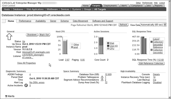
FIGURE 2-18. The home page for an Oracle instance in Enterprise Manager
FIGURE 2-19. Management areas for an Oracle database in Enterprise Manager
In terms of functionality, Enterprise Manager has now grown to the point where you can do practically anything with this tool that you can do with any other management tool, even basic command-line utilities. The screenshot shown in Figure 2-19 shows a simple list of the areas that you can view and modify for an Oracle database instance through Enterprise Manager.
In both of these figures, you can see another key facet of Enterprise Manager. The user interface for Enterprise Manager is browser-based, and much of the information displayed also acts as a link to more detail on the area summarized by the information. To show one more example, Figure 2-20 illustrates the type of detail you can get about a SQL query, which can be reached from many different pages that display information about SQL, from a historical listing to a list of the SQL statements that have used the most resources.
With this depth of functionality, Enterprise Manager has also greatly expanded the breadth of management coverage. With Enterprise Manager, you can now manage software in the middle tier, applications and business transactions, network performance, operating systems, and even some types of hardware.
FIGURE 2-20. SQL detail in Enterprise Manager
This last area of focus, hardware management, has been significantly expanded through the recent Sun acquisition. Sun’s management tool, Operations Center, is being integrated into the standard Enterprise Manager framework. Quite a few of Oracle’s acquisitions over the recent past have been components that are being integrated into the Enterprise Manager arena.
Enterprise Manager is even expanding its role in time, moving from managing a runtime IT environment to tools and helpers that can manage many parts of the software development process, including testing.
The capabilities of Enterprise Manager are so rich that no attempt to summarize them in a few pages would do justice to the product. Entire books have been written on the product, with more needed. For the purposes of this book, you should just understand that you will use Enterprise Manager to monitor and manage the activity of the Oracle software on the Exadata Database Machine in the same way that you would use Enterprise Manager with a standard Oracle database. Many scenarios on the Database Machine are no different from those of an individual instance. For example, if an ASM disk group goes down, Enterprise Manager recognizes this failure and can send an alert to an administrator. Whether this ASM group was built with disks on Exadata storage or not makes no difference in the way that Enterprise Manager will operate.
Enterprise Manager does include a plug-in that provides some extra capabilities relating only to the Database Machine, and the operation of this plug-in will be covered in the next chapter, as well as in Chapter 5.
Data Movement
The Exadata Database Machine is a real leap forward in performance and capability, and most customers already have a set of applications that can benefit from this new level of operation. Since these applications run on existing data stores, you will usually have to move data from those existing stores to the new platform.
Chapter 10 is focused on migration, but there are a few utilities and features of Oracle Database 11g that come into play when you are moving data onto the platform.
Utilities
Two basic utilities are used to move data into an Oracle Database. SQL*Loader is used to load data from standard external files into the database. SQL*Loader can be used to do more than simply put a complete file into a table, giving you the options to use multiple files as sources, multiple tables as targets, select the data to be loaded, and manipulate data being loaded through the use of SQL functions.
The other utility is Data Pump. Data Pump can export data from an Oracle database into a proprietary file format, which can be used as a source for the Data Pump import process. Data Pump can also load data directly from one Oracle database into another.
Best practices for the Exadata Database Machine call for the use of external tables for loads, rather than the use of these utilities, as described next.
Features
Three features of the Oracle database are also used in the process of moving data into an Oracle database. The first feature is used in conjunction with partitioning, which was discussed in a previous section. To move data into a partitioned table, you can create a temporary table with the same characteristics as a partitioned table and load the data into the table. Once the table is loaded, you create matching indexes on the table and calculate statistics on the table and its columns. At this point, you can add the table as a partition to the partition table target with a single operation, EXCHANGE PARTITION. This operation simply modifies the meta-data for the partitioned table, which causes a minimal interruption in production work.
As Exadata Database Machines are frequently used for data warehouse work, where large volumes of data are regularly added to existing databases, the EXCHANGE PARTITION method, along with the advantages of parallelism for loading, can come in handy.
Another feature that gives you the ability to add data to an existing Oracle database with very little interruption in service is the transportable tablespace. The tablespace is a logical storage unit that underlies all Oracle data structures.
Normally, when you migrate data, you have to extract data from the source database and load it into the target database. But transportable tablespaces, like the partition exchange explained previously, give you a faster way to migrate data from one Oracle database to another. With a transportable tablespace, you simply export the meta-data about the tablespace from the source database, move the files that are used by the tablespace to the target machine, and then load the meta-data into the data dictionary of the target machine.
You can even create a transportable tablespace from a backup set with Recovery Manager and have the tablespace reflect the state of the database at a specific point in time or SCN (system control number).
Finally, Oracle Database 11g includes a feature known as the Database File System, or DBFS. DBFS is built on SecureFiles, the feature used to store large objects, but builds on this storage capability by adding a file system interface, which allows a user to access the files through standard file system calls.
DBFS is used for moving data in conjunction with another Oracle feature known as external files. An external file, as the name implies, lives outside of the standard Oracle database. When you define an external table, you point to the external data source but create meta-data about that file, which allows users to access the file as if it were a table using standard SQL syntax.
One of the fastest ways to perform an actual import into Oracle tables is using a method known as CREATE TABLE AS SELECT . . ., or CTAS, which both creates a table using the structure defined by the SELECT statement and then loads the result set from the statement into the table.
TIP
You can use a similar method, INSERT AS APPEND, to add data to an existing table with similar benefits.
CTAS can use parallel execution to write data into tables very rapidly. Couple this with external tables, which can be read in parallel with the CTAS method, and you have an import method that takes full advantage of parallelism.
With DBFS, you can store external tables in the Oracle-based file system. This storage gives all the standard advantages of DBFS. Files stored in DBFS can be shared among multiple users of the Oracle database. File load operations are frequently performed using a RAC database as the target, which means that the source files have to be available on shared storage. Placing external tables in the DBFS meets this condition.
Operating Systems
Up until Oracle OpenWorld 2010, there wasn’t much to say about operating systems as they related to the Exadata Database Machine. But the event featured several announcements about the operating systems that support the Database Machine, which make this a topic worthy of some discussion.
Solaris Support
Oracle announced that they will support the Solaris operating system with the release of Solaris 11 Express, which should be available by the time you read this book. The X2-8 version of the Exadata Database Machine will come with both Solaris and Oracle Linux installed, and you can choose which operating system you want to run on the database server nodes when the Machine is installed.
In fact, you could even run Solaris on one node of the X2-8 and Oracle Linux on the other node of the X2-8, although you could not, of course, combine these nodes into a single RAC cluster if they were running different operating systems.
Oracle Linux
Oracle also announced that the newly renamed Oracle Linux will now support two different Linux kernels. One kernel is designed to be 100 percent compatible with Red Hat Linux. Another kernel, termed the Unbreakable Enterprise Kernel (UEK), includes a wide range of enhancements that contribute to significant performance gains, such as 1.8 times more OLTP transactions per second, as claimed by Oracle.
These enhancements were added to the Linux kernel in order to support the type of high-performance, modern components that make up the Exadata Database Machine. For instance, the UEK supports memory affinity, which ensures that a particular server node will use the co-located memory rather than memory on another node—a change that could mean a performance benefit of an order of magnitude. The Unbreakable Enterprise Kernel includes many other enhancements, such as better support for Infiniband and flash memory, which also contribute to improved performance.
You can choose either Linux kernel when you install Linux for the Exadata Database Machine, although the Unbreakable Linux Kernel will initially only be available for database nodes in the X2-8 version of the Database Machine. With the improved performance delivered by the new kernel, it is a natural choice for use on the X2-8 database nodes.
Please note that the features that make the Unbreakable Enterprise Linux Kernel different have all been submitted for inclusion in the open-source version of Linux. Oracle Linux, with either kernel, is still completely open source.
Other Oracle Database 11g Features
Oracle Database 11g is probably the most feature-rich database product available today. The main sections already described in this lengthy chapter cover some of the large areas of functionality that either contribute to the overall performance of the Exadata Database Machine or will be used as part of the implementation of the Database Machine. There are a few other features that also play a role in addressing the same issues as the Database Machine that deserve a brief explanation.
Materialized Views
Data warehouses are used to extract additional value from an organization’s data store by using that data for additional analysis. This analysis usually involves aggregation of the underlying data, a process that can take a significant amount of time in the production environment.
Materialized views are one way to reduce the runtime cost of these aggregations. A materialized view allows you to precalculate summary information, which not only avoids the need to perform these resource-intensive tasks at runtime, but also allows multiple queries looking for the same aggregation to reuse the same summaries. Materialized views come with their own set of refresh management options. You can choose to completely refresh the summaries in a materialized view, to perform an incremental refresh, or even to refresh summaries in materialized views every time an underlying table is updated. This last option gives you absolutely up-to-date summary information, but does impose overhead on every write operation to a table with one or more materialized views.
There are a set of views in the Oracle data dictionary that provide information on how much the data underlying a materialized view has changed, so you can determine if a materialized view needs a refresh based on this information.
Precomputed summaries can save runtime resources and enhance performance, and the flexible management of the refresh process is also a time-saver, but at this point you may wonder what is so special about materialized views. How is their functionality different from a summary table you build yourself?
The answer to this question lies with the Oracle optimizer. The optimizer recognizes the existence and composition of materialized views and can perform an operation known as query rewrite. When the optimizer receives a query requesting summary information that could be retrieved from a materialized view, the optimizer transparently rewrites the query to use this precomputed data. With query rewrite, you don’t have to modify any SQL in any application to take advantage of a materialized view.
Oracle OLAP
Oracle OLAP gives you the ability to embed complete OLAP cubes within the Oracle database. These cubes are managed just like any other data in an Oracle database, included in the same backup and recovery procedures and able to use the same security capabilities as the Oracle database. You can also access data in an Oracle OLAP cube with the same SQL as you use with a standard Oracle schema structure, with the different aspects of the cube being exposed as cube-views.
An Oracle OLAP cube, like a materialized view, contains precomputed summary information. And like materialized views, the summaries in the Oracle OLAP cube are used in the query rewrite process.
If you find yourself using a load of materialized views to precompute a large number of potential aggregates on the same set of tables, you might find that using an Oracle OLAP cube could lower your overall maintenance, since you can refresh all the cells in a cube with a single refresh operation.
Star Transformation
A star transformation is another type of query rewrite performed by the Oracle optimizer. The star transformation is performed as a way to significantly improve the performance of queries directed against a standard star schema, which includes a fact table and a large number of dimensions.
To understand how a star transformation works, consider the following query, typical in a data warehouse scenario:
Select SUM(quantity_sold)
From Sales s, Customers c, Products p, Times t
Where s.cust_id = c.cust_id
And s.prod_id = p.prod_id
And s.time_id = t.time_id
And c.cust_city ='BOSTON'
And p.product ='UMBRELLA'
And t.month ='MAY'
And t.year = 2008;
Normally, the optimizer would start out by looking to perform a four-way join in the most optimal way, between the SALES, CUSTOMERS, PRODUCTS, and TIMES tables. Although the dimension tables are much smaller than the SALES fact table, performing a multiple-way join can still be costly, especially since the point of the join is simply to use the Cartesian product of the dimensional join to identify the rows in the fact table for the SUM operation.
Before you can understand the true power of the star transformation, you will have to understand a type of index called a bitmap index. This index differs from a normal B*-tree index in that the bitmap index includes a string of bits that represent individual rows in the underlying table for each value in the index. If the index column in the row has a particular value, that bit is set to 1 (turned on) for that row in the string of bits for that index value. Bitmap indexes are particularly suited to data warehouse scenarios, where the cardinality of the index is very low.
The beauty of the bitmap is when the index is used for selection or joins. Because the values are indicated by individual bits, the server can use a bitwise operation to compare two bitmap indexes, and bitwise operations are extremely fast. So if you have a query that is looking to use multiple selection criteria and each of these criteria is represented in a bitmap index, the server simply does a few fast operations instead of multiple selection operations.
When a star transformation is performed, the optimizer recognizes that the targets of the query are tables that exist in a star schema, with a bitmap index on each of the dimension values. The optimizer rewrites the query to include subselects that take advantage of these bitmap indexes, resulting in this query:
Select SUM(quanity_sold)
From Sales s
Where s.cust_id IN
(Select c.cust_id From Customers c Where c.cust_city ='BOSTON')
And s.prod_id IN
(Select p.prod_id From Products p where p.product ='UMBRELLA')
And s.time_id IN
(Select t.time_id From Times t Where t.month ='MAY' And t.year = 2008);
The end result is an execution plan that is much faster than the execution plan that would have been required for the original query.
The query used in this example only uses the dimensions as a method to select rows from the fact table. But the optimizer can also use a star transformation to transform queries that need additional information from some or all of the dimension tables. The optimizer simply uses the interim result set from the star transformation as the driving table to join back to the dimension tables for the additional information. And, of course, the optimizer calculates the total cost of the star transformation versus the cost of running the query untouched to determine whether the star transformation will result in a faster execution plan.
Although star transformations are not unique to the Exadata Database Machine, this feature can provide significant performance benefits for data warehouse implementations on this platform.
Encryption
There is nothing about encryption as implemented in Oracle Database 11g software that is uniquely applicable to the Exadata Database Machine. Oracle Database 11g Advanced Security Option includes Transparent Data Encryption, so named because you can use this encryption without any changes to your application code. The encryption is implemented transparently.
However, the newest versions of the Oracle Database Machine use the X5600 (Westmere) chip in the Exadata Storage Server, as well as the database nodes in the X2-2 models. This chip supports AES-NI hardware-based encryption and decryption, which means these operations can be offloaded to these chips for much faster performance as well as relieving the database or storage server CPUs from the overhead of performing this task. Both the X2-2 database nodes and the storage server nodes will use this capability to decrypt data, with the goal of using the chip for encryption in future releases.
Since this capability is transparent, as is the encryption itself, you don’t really have to concern yourself with it, although this enhancement will help the Exadata Database Machine perform even better with encrypted data than before the advent of this hardware for offloading operations.
Summary
In this chapter, you learned about the foundation that the features of Oracle Database 11g provided for Exadata technology. These capabilities have been built up over decades of development and include these major features:
![]() Multiversion read consistency, which prevents locking contention between writers and readers, removing one of the key factors in performance degradation
Multiversion read consistency, which prevents locking contention between writers and readers, removing one of the key factors in performance degradation
![]() Real Application Clusters, which allow you to increase the horsepower and availability of your Oracle database by combining multiple database server nodes into a single Oracle database
Real Application Clusters, which allow you to increase the horsepower and availability of your Oracle database by combining multiple database server nodes into a single Oracle database
![]() Automated Storage Management, which delivers complete volume and storage management, providing scalability, performance, and reliability for database storage
Automated Storage Management, which delivers complete volume and storage management, providing scalability, performance, and reliability for database storage
![]() Partitioning, which helps to eliminate portions of data from consideration in supplying results to queries, a precursor to some of the features in Exadata software
Partitioning, which helps to eliminate portions of data from consideration in supplying results to queries, a precursor to some of the features in Exadata software
![]() Parallel execution, which allows the use of multiple CPUs to address the needs of individual tasks and subtasks that are part of a SQL request, delivering greater performance in some scenarios and environments
Parallel execution, which allows the use of multiple CPUs to address the needs of individual tasks and subtasks that are part of a SQL request, delivering greater performance in some scenarios and environments
![]() Data Guard, which provides a disaster-resilient configuration to provide for the highest levels of availability
Data Guard, which provides a disaster-resilient configuration to provide for the highest levels of availability
![]() Compression, which is available in different flavors in Oracle Database 11g and an additional variety in Exadata
Compression, which is available in different flavors in Oracle Database 11g and an additional variety in Exadata
![]() Database Resource Manager, which is used to allocate oversubscribed resources among different groups of database users
Database Resource Manager, which is used to allocate oversubscribed resources among different groups of database users
![]() A variety of other features and functionality used in the Exadata world, including Enterprise Manager for management, tools for data movement, and different operating systems used on the Exadata Database Machine
A variety of other features and functionality used in the Exadata world, including Enterprise Manager for management, tools for data movement, and different operating systems used on the Exadata Database Machine
This extensive list demonstrates that Exadata technology did not spring from the Oracle development organization as an entirely new entity, but rather as a continuation of progress that has been going on since the early days of Oracle.
The next chapter will cover the software that is unique to the Exadata Database Machine.
All materials on the site are licensed Creative Commons Attribution-Sharealike 3.0 Unported CC BY-SA 3.0 & GNU Free Documentation License (GFDL)
If you are the copyright holder of any material contained on our site and intend to remove it, please contact our site administrator for approval.
© 2016-2026 All site design rights belong to S.Y.A.