Pig Design Patterns (2014)
Chapter 1. Setting the Context for Design Patterns in Pig
This chapter is aimed at providing a broad introduction to multiple technologies and concepts addressed in this book. We start with exploring the concepts related to design patterns by defining them and understanding how they are discovered and applied in real life, and through this, we seek to understand how these design patterns are applied and implemented in Pig.
Before we start looking into the intricacies of the Pig programming language, we explore the background of why Pig came into existence, where Pig is used in an enterprise, and understand how Hadoop fits in the distributed computing landscape in the age of Big Data. We then perform a quick dive into the Hadoop ecosystem, introducing you to its important features. The Pig programming language has been covered from the language features perspective, giving you a ready-made example that is elaborated to explain the language features, such as common operators, extensibility, input and output operators, relational operators, schemas, nulls, and ways to understand the intermediate MapReduce code.
Understanding design patterns
Design patterns provide a consistent and common solutions approach to similar problems or requirements. A designer working with diverse systems often comes across a similarity in the way a problem manifests itself or a requirement that needs to be met. Eventually, he/she gains enough knowledge of the subtle variations, and starts seeing a common thread connecting these otherwise different and recurring problems. Such common behavior or characteristics are then abstracted into a pattern. This pattern or solution approach is thus a generalized design that can also be applied to a broader set of requirements and newer manifestations of the problem. For example, the widely acclaimed software design patterns book, Design Patterns: Elements of Reusable Object-Oriented Software by Erich Gamma, Richard Helm, Ralph Johnson, and John Vlissides, Addison-Wesley Professional, mentions five creational patterns. These patterns can also be understood by analyzing real-life situations that trace their origin to a non-software field. The factory method pattern mentioned in this book defines an interface for the creation of class objects, but it lets the subclasses perform the decision making on which class to instantiate. This software pattern seems to have a parallel in the non-software industry where toys are manufactured by the injection molding process. The machine processes the plastic powder and injects the powder into molds of the required shapes. The class of the toy (car, action figure, and so on) is determined by its mold.
The intent of the design pattern is not to act like a perfect tailor-made solution for a specific problem that can be converted into code. Rather, it is like a template to solve specific and well-defined problems. Usually, design patterns are uncovered in real life; they are not created. The following are general ways in which patterns are discovered:
· The evolution of a new group of technologies that solve the latest problems together; these technologies have a perceived need for a pattern catalog
· Encountering a solution that has recurring problems
Adapt the existing patterns to new situations and modify the existing pattern itself. Discovering a pattern implies defining it, giving it a name, and documenting it in a very clear way so that users can read, understand, and apply them when faced with similar problems. A pattern is worth publishing after it is used by real users and they have worked on real-world problems rather than hypothetical issues. These patterns are not rules or laws; they are guidelines that may be modified to fit the needs of the solution.
This book takes inspiration from other books written on design patterns on various subject areas. It also follows the pattern documentation format as outlined by the GoF pattern catalog Design Patterns: Elements of Reusable Object-Oriented Software, by Gamma,Helm, Johnson & Vlissides (Addison-Wesley Professional).
Every design pattern in this book follows a template and is identified by a name, followed by a few sections that tell the user more about the patterns.
· The pattern name gives the pattern a unique identifier and can be a good means of communication.
· The pattern details section succinctly describes the what and why of the pattern.
· The Background section describes the motivation and in-detail applicability of the pattern.
· The Motivation section describes a concrete scenario that describes the problem and how the pattern fits as a solution. Applicability describes different situations where the pattern is used.
· The Use cases section deals with various use cases in real systems where we can see evidence of the pattern.
· The Code snippets section consists of the code through which the pattern is implemented.
· The Results section has the consequences of the pattern that deal with the intended and unintended effect of the output of the pattern.
· The Additional information section deals with how the patterns relate to each other, and any other relevant information related to the pattern.
You apply a pattern when you identify a problem, which a pattern can solve, and recognize the similarity to other problems that might be solved using known patterns. This can happen during the initial design, coding, or maintenance phase. In order to do this, you need to get familiar with the existing patterns and their interrelationships first, and then look at the Background section that delves deeper into the motivation and applicability of the pattern for the design problem.
The scope of design patterns in Pig
This book deals with patterns that were encountered while solving real-world, recurrent Big Data problems in an enterprise setting. The need for these patterns takes root in the evolution of Pig to solve the emerging problems of large volumes and a variety of data, and the perceived need for a pattern catalog to document their solutions.
The emerging problems of handling large volumes of data, typically deal with getting a firm grip on understanding whether the data can be used or not to generate analytical insights and, if possible, how to efficiently generate these insights. Imagine yourself to be in the shoes of a data scientist who has been given a massive volume of data that does not have a proper schema, is messy, and has not been documented for ages. You have been asked to integrate this with other enterprise data sources and generate spectacular analytical insights. How do you start? Would you start integrating data and fire up your favorite analytics sandbox and begin generating results? Would it be handy if you knew beforehand the existence of design patterns that can be applied systematically and sequentially in this kind of scenario to reduce the error and increase the efficiency of Big Data analytics? The design patterns discussed in this book will definitely appeal to you in this case.
Design patterns in Pig are geared to enhance your ability to take a problem of Big Data and quickly apply the patterns to solve it. Successful development of Big Data solutions using Pig requires considering issues early in the lifecycle of development, and these patterns help to uncover those issues. Reusing Pig design patterns helps identify and address such subtleties and prevents them from growing into major problems. The by-product of the application of the patterns is readability and maintainability of the resultant code. These patterns provide developers a valuable communication tool by allowing them to use a common vocabulary to discuss problems in terms of what a pattern could solve, rather than explaining the internals of a problem in a verbose way. Design patterns for Pig are not a cookbook for success; they are a rule of thumb. Reading specific cases in this book about Pig design patterns may help you recognize problems early, saving you from the exponential cost of reworks later on.
The popularity of design patterns is very much dependent on the domain. For example, the state patterns, proxies, and facades of the Gang of Four book are very common with applications that communicate a lot with other systems. In the same way, the enterprises, which consume Big Data to understand analytical insights, use patterns related to solving problems of data pipelines since this is a very common use case. These patterns specifically elaborate the usage of Pig in data ingest, profiling, cleansing, transformation, reduction, analytics, and egress.
A few patterns discussed in Chapter 5, Data Transformation Patterns and Chapter 6, Understanding Data Reduction Patterns, adapt the existing patterns to new situations, and in the process modify the existing pattern itself. These patterns deal with the usage of Pig in incremental data integration and creation of quick prototypes.
These design patterns also go deeper and enable you to decide the applicability of specific language constructs of Pig for a given problem. The following questions illustrate this point better:
· What is the recommended usage of projections to solve specific patterns?
· In which pattern is the usage of scalar projections ideal to access aggregates?
· For which patterns is it not recommended to use COUNT, SUM, and COUNT_STAR?
· How to effectively use sorting in patterns where key distributions are skewed?
· Which patterns are related to the correct usage of spill-able data types?
· When not to use multiple FLATTENS operators, which can result in CROSS on bags?
· What patterns depict the ideal usage of the nested FOREACH method?
· Which patterns to choose for a JOIN operation when one dataset can fit into memory?
· Which patterns to choose for a JOIN operation when one of the relations joined has a key that dominates?
· Which patterns to choose for a JOIN operation when two datasets are already ordered?
Hadoop demystified – a quick reckoner
We will now discuss the need to process huge multistructured data and the challenges involved in processing such huge data using traditional distributed applications. We will also discuss the advent of Hadoop and how it efficiently addresses these challenges.
The enterprise context
The last decade has been a defining moment in the history of data, resulting in enterprises adopting new business models and opportunities piggybacking on the large-scale growth of data.
The proliferation of Internet searches, personalization of music, tablet computing, smartphones, 3G networks, and social media contributed to the change in rules of data management, from organizing, acquiring, storing, and retrieving data to managing perspectives. The need for decision making for these new sources of data and getting valuable insights has become a valuable weapon in the enterprise arsenal, aimed to make the enterprise successful.
Traditional systems, such as RDBMS-based data warehouses, took the lead to support the decision-making process by being able to collect, store, and manage data by applying traditional and statistical methods of measurement to create a reporting and analysis platform. The data collected within these traditional systems were highly structured in nature with minimal flexibility to change with the needs of the emerging data types, which were more unstructured.
These data warehouses are capable of supporting distributed processing applications, but with many limitations. Such distributed processing applications are generally oriented towards taking in structured data, transforming it, and making it usable for analytics or reporting, and these applications were predominantly batch jobs. In some cases, these applications are run on a cluster of machines so that the computation and data are distributed to the nodes of the cluster. These applications take a chunk of data, perform a computationally intense operation on it, and send it to downstream systems for another application or system to consume.
With the competitive need to analyze both structured and unstructured data and gain insights, the current enterprises need the processing to be done on an unprecedentedly massive scale of data. The processing mostly involves performing operations needed to clean, profile, and transform unstructured data in combination with the enterprise data sources so that the results can be used to gain useful analytical insights. Processing these large datasets requires many CPUs, sufficient I/O bandwidth, Memory, and so on. In addition, whenever there is large-scale processing, it implies that we have to deal with failures of all kinds. Traditional systems such as RDBMS do not scale linearly or cost effectively under this kind of tremendous data load or when the variety of data is unpredictable.
In order to process the exceptional influx of data, there is a palpable need for data management technology solutions; this allows us to consume large volumes of data in a short amount of time across many formats, with varying degrees of complexity to create a powerful analytical platform that supports decisions.
Common challenges of distributed systems
Before the genesis of Hadoop, distributed applications were trying to cope with the challenges of data growth and parallel processing in which processors, network, and storage failure was common. The distributed systems often had to manage the problems of failure of individual components in the ecosystem, arising out of low disk space, corrupt data, performance degradations, routing issues, and network congestion. Achieving linear scalability in traditional architectures was next to impossible and in cases where it was possible to a limited extent, it was not without incurring huge costs.
High availability was achieved, but at a cost of scalability or compromised integrity. The lack of good support for concurrency, fault tolerance, and data availability were unfavorable for traditional systems to handle the complexities of Big Data. Apart from this, if we ever want to deploy a custom application, which houses the latest predictive algorithm, distributed code has its own problems of synchronization, locking, resource contentions, concurrency control, and transactional recovery.
Few of the previously discussed problems of distributed computing have been handled in multiple ways within the traditional RDBMS data warehousing systems, but the solutions cannot be directly extrapolated to the Big Data situation where the problem is amplified exponentially due to huge volumes of data, and its variety and velocity. The problems of data volume are solvable to an extent. However, the problems of data variety and data velocity are prohibitively expensive to be solved by these attempts to rein in traditional systems to solve Big Data problems.
As the problems grew with time, the solution to handle the processing of Big Data was embraced by the intelligent combination of various technologies, such as distributed processing, distributed storage, artificial intelligence, multiprocessor systems, and object-oriented concepts along with Internet data processing techniques
The advent of Hadoop
Hadoop, a framework that can tolerate machine failure, is built to outlast challenges concerning the distributed systems discussed in the previous section. Hadoop provides a way of using a cluster of machines to store and process, in parallel, extremely huge amounts of data. It is a File System-based scalable and distributed data processing architecture, designed and deployed on a high-throughput and scalable infrastructure.
Hadoop has its roots in Google, which created a new computing model built on a File System, Google File System (GFS), and a programming framework, MapReduce, that scaled up the search engine and was able to process multiple queries simultaneously.Doug Cutting and Mike Cafarella adapted this computing model of Google to redesign their search engine called Nutch. This eventually led to the development of Nutch as a top-level Apache project under open source, which was adopted by Yahoo in 2006 and finally metamorphosed into Hadoop.
The following are the key features of Hadoop:
· Hadoop brings the power of embarrassingly massive parallel processing to the masses.
· Through the usage of File System storage, Hadoop minimizes database dependency.
· Hadoop uses a custom-built distributed file-based storage, which is cheaper compared to storing on a database with expensive storages such as Storage Area Network (SAN) or other proprietary storage solutions. As data is distributed in files across the machines in the cluster, it provides built-in redundancy using multinode replication.
· Hadoop's core principle is to use commodity infrastructure, which is linearly scalable to accommodate infinite data without degradation of performance. This implies that every piece of infrastructure, be it CPU, memory, or storage, added will create 100 percent scalability. This makes data storage with Hadoop less costly than traditional methods of data storage and processing. From a different perspective, you get processing done for every TB of storage space added to the cluster, free of cost.
· Hadoop is accessed through programmable Application Programming Interfaces (APIs) to enable parallel processing without the limitations imposed by concurrency. The same data can be processed across systems for different purposes, or the same code can be processed across different systems.
· The use of high-speed synchronization to replicate data on multiple nodes of the cluster enables a fault-tolerant operation of Hadoop.
· Hadoop is designed to incorporate critical aspects of high availability so that the data and the infrastructure are always available and accessible by users.
· Hadoop takes the code to the data rather than the other way round; this is called data locality optimization. This local processing of data and storage of results on the same cluster node minimizes the network load gaining overall efficiencies.
· To design fault tolerant applications, the effort involved to add the fault tolerance part is sometimes more than the effort involved in solving the actual data problem at hand. This is where Hadoop scores heavily. It enables the application developer to worry about writing applications by decoupling the distributed system's fault tolerance from application logic. By using Hadoop, the developers no longer deal with the low-level challenges of failure handling, resource management, concurrency, loading data, allocating, and managing the jobs on the various nodes in the cluster; they can concentrate only on creating applications that work on the cluster, leaving the framework to deal with the challenges.
Hadoop under the covers
Hadoop consists of the Hadoop core and Hadoop subprojects. The Hadoop core is essentially the MapReduce processing framework and the HDFS storage system.
The integral parts of Hadoop are depicted in the following diagram:
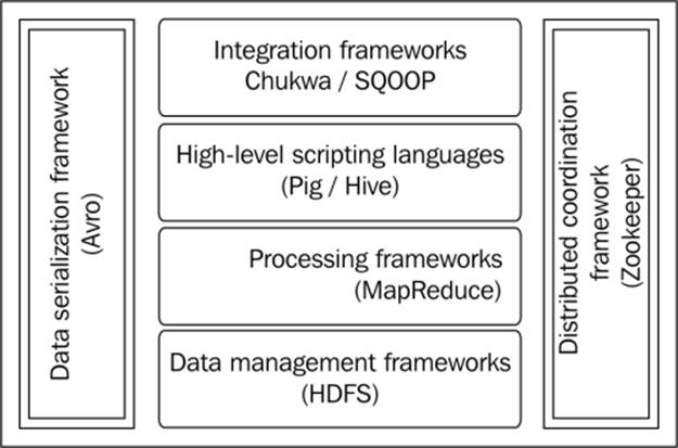
Typical Hadoop stack
The following is an explanation of the integral parts of Hadoop:
· Hadoop Common: This includes all the library components and utilities that support the ecosystem
· Hadoop Distributed File System (HDFS): This is a filesystem that provides highly available redundant distributed data access for processing using MapReduce
· Hadoop MapReduce: This is a Java-based software framework to operate on large datasets on a cluster of nodes, which store data (HDFS)
Few Hadoop-related top level Apache projects include the following systems:
· Avro: This a data serialization and deserialization system
· Chukwa: This is a system for log data collection
· SQOOP: This is a structured data collection framework that integrates with RDBMS
· HBase: This is a column-oriented scalable, distributed database that supports millions of rows and columns to store and query in real-time structured data using HDFS
· Hive: This is a structured data storage and query infrastructure built on top of HDFS, which is used mainly for data aggregation, summarization, and querying
· Mahout: This is a library of machine-learning algorithms written specifically for execution on the distributed clusters
· Pig: This is a data-flow language and is specially designed to simplify the writing of MapReduce applications
· ZooKeeper: This is a coordination service designed for distributed applications
Understanding the Hadoop Distributed File System
The Hadoop Distributed File System (HDFS) is a File System that provides highly available redundant data access to process using MapReduce. The HDFS addresses two major issues in large-scale data storage and processing. The first problem is that of data locality in which code is actually sent to the location of the data in the cluster, where the data has already been divided into manageable blocks so that each block can be independently processed and the results combined. The second problem deals with the capability to tolerate faults at any subsystem level (it can be at the CPU, network, storage, memory, or application level) owing to the reliance on commodity hardware, which is assumed to be less reliant, unless proven otherwise. In order to address these problems, the architecture of HDFS was inspired by the early lead taken by the GFS.
HDFS design goals
The three primary goals of HDFS architecture are as follows:
· Process extremely large files ranging from multiple gigabytes to petabytes.
· Streaming data processing to read data at high-throughput rates and process data while reading.
· Capability to execute on commodity hardware with no special hardware requirements.
Working of HDFS
HDFS has two important subsystems. One is NameNode, which is the master of the system that maintains and manages the blocks that are present in the other nodes. The second one is DataNodes, which are slave nodes working under the supervision of the NameNode and deployed on each machine to provide the actual storage. These nodes collectively serve read and write requests for the clients, which store and retrieve data from them. This is depicted in the following diagram:
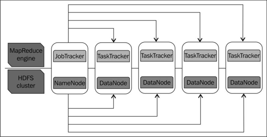
JobTracker and NameNode
The master node is the place where the metadata of the data splits is stored in the memory. This metadata is used at a later point in time to reconstruct the complete data stored in the slave nodes, enabling the job to run on various nodes. The data splits are replicated on a minimum of three machines (the default replication factor). This helps in situations when the hardware of the slave nodes fails and the data can be readily recoverable from the machines where the redundant copy was stored, and the job was executed on one of those machines. Together, these two account for the storage, replication, and management of the data in the entire cluster.
On a Hadoop cluster, the data within the filesystem nodes (data nodes) are replicated on multiple nodes in the cluster. This replication adds redundancy to the system in case of machine or subsystem failure; the data stored in the other machines will be used for the continuation of the processing step. As the data and processing coexist on the same node, linear scalability can be achieved by simply adding a new machine and gaining the benefit of an additional hard drive and the computation capability of the new CPU (scale out).
It is important to note that HDFS is not suitable for low-latency data access, or storage of many small files, multiple writes, and arbitrary file modifications.
Understanding MapReduce
MapReduce is a programming model that manipulates and processes huge datasets; its origin can be traced back to Google, which created it to solve the scalability of search computation. Its foundations are based on principles of parallel and distributed processing without any database dependency. The flexibility of MapReduce lies in its ability to process distributed computations on large amounts of data in clusters of commodity servers, with a facility provided by Hadoop and MapReduce called data locality, and a simple task-based model for management of the processes.
Understanding how MapReduce works
MapReduce primarily makes use of two components; a JobTracker, which is a Master node daemon, and the TaskTrackers, which run in all the slave nodes. It is a slave node daemon. This is depicted in the following diagram:
MapReduce internals
The developer writes a job in Java using the MapReduce framework, and submits it to the master node of the cluster, which is responsible for processing all the underlying data with the job.
The master node consists of a daemon called JobTracker, which assigns the job to the slave nodes. The JobTracker class, among other things, is responsible for copying the JAR file containing the task on to the node containing the task tracker so that each of the slave node spawns a new JVM to run the task. The copying of the JAR to the slave nodes will help in situations that deal with slave node failure. A node failure will result in the master node assigning the task to another slave node containing the same JAR file. This enables resilience in case of node failure.
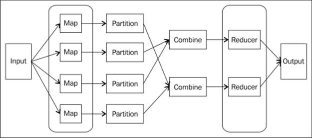
The MapReduce internals
A MapReduce job is implemented as two functions:
· The Map function: A user writes a Map function, which receives key-value pairs as input, processes it, and emits a list of key-value pairs.
· The Reduce function: The Reduce function, written by the user, will accept the output of the Map function, that is, the list of intermediate key-value pairs. These values would be typically merged to form a smaller set of values and hence the name Reduce. The output could be just zero or one output value per each reducer invocation.
The following are the other components of the MapReduce framework as depicted in the previous diagram:
· Combiner: This is an optimization step and is invoked optionally. It is a function specified to execute a Reduce-like processing on the Mapper side and perform map-side aggregation of the intermediate data. This will reduce the amount of data transferred over the network from the Mapper to the Reducer.
· Partitioner: This is used to partition keys of the map output. The key is used to develop a partition by grouping all values of a key together in a single partition. Sometimes default partitions can be created by a hash function.
· Output: This collects the output of Mappers and Reducers.
· Job configuration: This is the primary user interface to manage MapReduce jobs to specify the Map, Reduce functions, and the input files.
· Job input: This specifies the input for a MapReduce job.
Pig – a quick intro
Pig is MapReduce simplified. It is a combination of the Pig compiler and the Pig Latin script, which is a programming language designed to ease the development of distributed applications for analyzing large volumes of data. We will refer to the whole entity as Pig.
The high-level language code written in the Pig Latin script gets compiled into sequences of the MapReduce Java code and it is amenable to parallelization. Pig Latin promotes the data to become the main concept behind any program written in it. It is based on the dataflow paradigm, which works on a stream of data to be processed; this data is passed through instructions, which processes the data. This programming style is analogous to how electrical signals flow through circuits or water flows through pipes.
This dataflow paradigm is in stark contrast to the control flow language, which works on a stream of instructions, and operates on external data. In a traditional program, the conditional executions, jumps, and procedure calls change the instruction stream to be executed.
Processing statements in Pig Latin consist of operators, which take inputs and emit outputs. The inputs and outputs are structured data expressed in bags, maps, tuples, and scalar data. Pig resembles a dataflow graph, where the directed vertices are the paths of data and the nodes are operators (such as FILTER, GROUP, and JOIN) that process the data. In Pig Latin, each statement executes as soon as all data reaches them in contrast to a traditional program that executes as soon as it encounters the statement.
A programmer writes code using a set of standard data-processing Pig operators, such as JOIN, FILTER, GROUP BY, ORDER BY, and UNION. These are then translated into MapReduce jobs. Pig itself does not have the capability to run these jobs and it delegates this work to Hadoop. Hadoop acts as an execution engine for these MapReduce jobs.
It is imperative to understand that Pig is not a general purpose programming language with all the bells and whistles that come with it. For example, it does not have the concept of control flow or scope resolution, and has minimal variable support, which many developers are accustomed to in traditional languages. This limitation can be overcome by using User Defined Functions (UDFs), which is an extensibility feature of Pig.
For a deeper understanding, you may have to refer the Apache web site at http://pig.apache.org/docs/r0.11.0/ to understand the intricacies of the syntax, usage, and other language features.
Understanding the rationale of Pig
Pig Latin is designed as a dataflow language to address the following limitations of MapReduce:
· The MapReduce programming model has tightly coupled computations that can be decomposed into map phase, shuffle phase, and a reducer phase. This limitation is not appropriate for real-world applications that do not fit into this pattern and tasks having a different flow like joins or n-phases. Few other real-world data pipelines require additional coordination code to combine separate MapReduce phases for management of the intermediate results between pipeline phases. This takes its toll in terms of the learning curve for new developers to understand the computation.
· Complex workarounds have to be implemented in MapReduce even for the simplest of operations like projection, filtering, and joins.
· The MapReduce code is difficult to develop, maintain, and reuse, sometimes taking the order of the magnitude than the corresponding code written in Pig.
· It is difficult to perform optimizations in MapReduce because of its implementation complexity.
Pig Latin brings the double advantage of being a SQL-like language with its declarative style and the power of a procedural programming language such as MapReduce using various extensibility features.
Pig supports nested data and enables complex data types to be embedded as fields of a table. The support for nested data models makes data modeling more intuitive since this is closer to the reality of how data exists than the way a database models it in the first normal form. The nested data model also reflects how the data is stored on the disk and enables users to write custom UDFs more intuitively.
Pig supports creation of user-defined functions, which carry out specialized data processing tasks; almost all aspects of programming in Pig are extensible using UDFs. What it implies is that a programmer can customize Pig Latin functions like grouping, filtering, and joining using the EvalFunc method. You can also customize load/store capabilities by extending LoadFunc or StoreFunc. Chapter 2, Data Ingest and Egress Patterns, has examples showing Pig's extensibility.
Pig has a special feature, called the ILLUSTRATE function to aid the Big Data developer to develop code using sample data quickly. The sample data closely resembles the real data as much as possible and fully illustrates the semantics of the program. This example data evolves automatically as the program grows in complexity. This systematic example data can help in detecting errors and its sources early.
One other advantage of using Pig is that there is no need to perform an elaborate data import process prior to parsing the data into tuples as in conventional database management systems. What it implies is, if you have a data file, the Pig Latin queries can be run on it directly without importing it. Without importing means that the data can be accessed and queried in any format as long as it can be read by Pig as tuples. We don't need to import data as we do it while working with a database, for example, importing a CSV file into a database before querying it. Still, you need to provide a function to parse the content of the file into tuples.
Understanding the relevance of Pig in the enterprise
In the current enterprises, the Big Data processing cycle is remarkable for its complexity and it widely differs from a traditional data processing cycle. The data collected from a variety of data sources is loaded to a target platform; then a base level analysis is performed so that a discovery happens through a metadata layer being applied to the data. This will result in the creation of a data structure or schema for the content in order to discover the context and relevance of the data. Once the data structure is applied, the data is then integrated, transformed, aggregated, and prepared to be analyzed. This reduced and structured dataset is used for reporting and ad hoc analytics. The result from the process is what provides insights into the data and any associated context (based on the business rules processed). Hadoop can be used as a processing and storage framework at each of the stages.
The following diagram shows a typical Big Data processing flow:
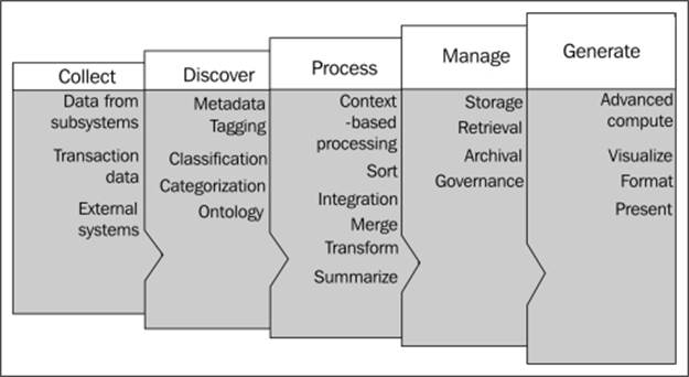
Big Data in the enterprise
The role of Pig as per the preceding diagram is as follows:
· In the collect phase, Pig is used to interface with the acquired data from multiple sources including real-time systems, near-real-time systems, and batch-oriented applications. Another way to use Pig is to process the data through a knowledge discovery platform, which could be upstream and store the subset of the output rather than the whole dataset.
· Pig is used in the data discovery stage where Big Data is first analyzed and then processed. It is in this stage that Big Data is prepared for integration with the structured analytical platforms or the data warehouse. The discovery and analysis stage consists of tagging, classification, and categorization of data, which closely resembles the subject area and results in the creation of data model definition or metadata. This metadata is the key to decipher the eventual value of Big Data through analytical insights.
· Pig is used in the data processing phase, where the context of the data is processed to explore the relevance of the data within the unstructured environment; this relevance would facilitate the application of appropriate metadata and master data in Big Data. The biggest advantage of this kind of processing is the ability to process the same data for multiple contexts, and then looking for patterns within each result set for further data mining and data exploration. For example, consider the word "cold", the context of the word has to be ascertained correctly based on the usage, semantics, and other relevant information. This word can be related to the weather or to a common disease. After getting the correct context for this word, further master data related to either weather or common diseases can be applied on the data.
· In the processing phase, Pig can also be used to perform data integration right after the contextualization of data, by cleansing and standardizing Big Data with metadata, master data, and semantic libraries. This is where the data is linked with the enterprise dataset. There are many techniques to link the data between structured and unstructured datasets with metadata and master data. This process is the first important step in converting and integrating the unstructured and raw data into a structured format. This is the stage where the power of Pig is used extensively for data transformation, and to augment the existing enterprise data warehouse by offloading high volume, low value data, and workloads from the expensive enterprise data warehouse.
· As the processing phase in an enterprise is bound by tight SLAs, Pig, being more predictable and having the capability to integrate with other systems, makes it more suitable to regularly schedule data cleansing, transformation, and reporting workloads.
Pig scores in situations where incoming data is not cleansed and normalized. It gracefully handles situations where data schemas are unknown until runtime or are inconsistent. Pig's procedural language model and schema-less approach offers much more flexibility and efficiency in data access so that data scientists can build research models on the raw data to quickly test a theory.
Pig is typically used in situations where the solution can be expressed as a Directed Acyclic Graph (DAG), involving the combination of standard relational operations of Pig (join, aggregation, and so on) and utilizing custom processing code via UDFs written in Java or a scripting language. This implies that if you have a very complex chain of tasks where the outputs of each job feeds as an input to the next job, Pig makes this process of chaining the jobs easy to accomplish.
Pig is useful in Big Data workloads where there is one very large dataset, and processing on that dataset includes constantly adding in new small pieces of data that will change the state of the large dataset. Pig excels in combining the newly arrived data so that the whole of the data is not processed, but only the delta of the data along with the results of the large data is processed efficiently. Pig provides operators that perform this incremental processing of data in a reasonable amount of time.
Other than the previously mentioned traditional use cases where Pig is generally useful, Pig has the inherent advantage in the form of much less development time needed to write and optimize code than to write in Java MapReduce. Pig is a better choice when performing optimization-by-hand is tedious. Pig's extensibility capabilities, through which you can integrate your existing executable and UDFs with Pig Latin scripts, enables even faster development cycles.
Working of Pig – an overview
This subsection is where an example Pig script gets dissected threadbare and is explained to illustrate the language features of Pig.
Firing up Pig
This subsection helps you to get a very quick understanding of booting Pig into the action mode by installing and configuring it.
The primary prerequisite for Pig to work in a Hadoop cluster is to maintain the Hadoop version compatibility, which in essence means Pig 0.11.0 works with Hadoop versions 0.20.X, 1.X, 0.23.X, and 2.X. This is done by changing the directory for HADOOP_HOME. The following table shows version compatibility between Apache Pig and Hadoop.
The following table summarizes the Pig versus Hadoop compatibility:
|
Apache Pig Version |
Compatible Hadoop Versions |
|
0.12.0 |
0.20.x, 1.x, 0.23.x, 2.x |
|
0.11.0 |
0.20.x, 1.x, 0.23.x, 2.x |
|
0.10.1 |
0.20.x, 1.x, 0.23.x, 2.x |
|
0.10.0 |
0.20.x, 1.0.x, 0.23.x |
|
0.9.2 |
0.20, 1.0.0 |
|
0.9.1 |
0.2 |
|
0.9.0 |
0.2 |
|
0.8.1 |
0.2 |
|
0.8.0 |
0.2 |
|
0.7.0 |
0.2 |
|
0.6.0 |
0.2 |
|
0.5.0 |
0.2 |
|
0.4.0 |
0.18 |
|
0.3.0 |
0.18 |
|
0.2.0 |
0.18 |
|
0.1.1 |
0.18 |
|
0.1.0 |
0.17 |
Pig core is written in Java and it works across operating systems. Pig's shell, which executes the commands from the user, is a bash script and requires a UNIX system. Pig can also be run on Windows using Cygwin and Perl packages.
Java 1.6 is also mandatory for Pig to run. Optionally, the following can be installed on the same machine: Python 2.5, JavaScript 1.7, Ant 1.7, and JUnit 4.5. Python and JavaScript are for writing custom UDFs. Ant and JUnit are for builds and unit testing, respectively. Pig can be executed with different versions of Hadoop by setting HADOOP_HOME to point to the directory where we have installed Hadoop. If HADOOP_HOME is not set, Pig will run with the embedded version by default, which is currently Hadoop 1.0.0.
The following table summarizes the prerequisites for installing Pig (we have considered major versions of Pig until 0.9.1):
|
Apache Pig Version |
Prerequisites |
|
0.12.0 |
Hadoop 0.20.2, 020.203, 020.204, 0.20.205, 1.0.0, 1.0.1, or 0.23.0, 0.23.1 |
|
Java 1.6 |
|
|
Cygwin(for windows) |
|
|
Perl(for windows) |
|
|
0.11.0,0.11.1 |
Hadoop 0.20.2, 020.203, 020.204, 0.20.205, 1.0.0, 1.0.1, or 0.23.0, 0.23.1 |
|
Java 1.6 |
|
|
Cygwin(for windows) |
|
|
Perl(for windows) |
|
|
0.10.0,0.10.1 |
Hadoop 0.20.2, 020.203, 020.204, 0.20.205, 1.0.0, 1.0.1, or 0.23.0, 0.23.1 |
|
Java 1.6 |
|
|
Cygwin(for windows) |
|
|
Perl(for windows) |
|
|
0.9.2 |
Hadoop 0.20.2, 0.20.203, 0.20.204, 0.20.205, or 1.0.0 |
|
Java 1.6 |
|
|
Cygwin(for windows) |
|
|
Perl(for windows) |
|
|
0.9.1 |
Hadoop 0.20.2, 0.20.203, 0.20.204 or 0.20.205 |
|
Java 1.6 |
|
|
Cygwin(for windows) |
|
|
Perl(for windows) |
Pig is typically installed in a machine, which is not a part of the Hadoop cluster. This can be a developer's machine, which has connectivity to the Hadoop cluster. This machine is called a gateway or edge machine.
The installation of Pig is a straightforward process. Download Pig from your favorite distribution site, be it Apache, Cloudera, or Hortonworks and follow the instructions specified in the installation guide specific to the distribution. These instructions generally involve steps to untar the tarball in a directory of your choice and setting the only configuration required, which is the JAVA_HOME property to the location that contains the Java distribution.
To verify if Pig was indeed installed correctly, try the command $ pig -help.
Pig can be run in two modes: local and MapReduce.
· The local mode: To run Pig in the local mode, install this mode on a machine where Pig is run using your local File System. The -x local flag is used to denote the local mode ($ pig -x local ...). The result of this command is the Pig shell called Grunt where you can execute command lines and scripts. The local mode is useful when a developer wants to prototype, debug, or use small data to quickly perform a proof of concept locally and then apply the same code on a Hadoop cluster (the MapReduce mode).
· $ pig -x local
· ... - Connecting to ...
grunt>
Tip
Downloading the example code
You can download the example code files for all Packt books you have purchased from your account at http://www.packtpub.com. If you purchased this book elsewhere, you can visit http://www.packtpub.com/support and register to have the files e-mailed directly to you.
· The MapReduce mode: This mode is used when you need to access a Hadoop cluster and run the application on it. This is the default mode and you can specify this mode using the -x flag ($ pig or $ pig -x mapreduce). The result of this command is the Pig shell called Grunt where you can execute commands and scripts.
· $ pig -x mapreduce
· ... - Connecting to ...
grunt>
You can also perform the following code snippet instead of the previous one:
$ pig
... - Connecting to ...
grunt>
It is important to understand that in both the local and MapReduce modes, Pig does the parsing, checking, compiling, and planning locally. Only the job execution is done on the Hadoop cluster in the MapReduce mode and on the local machine in the local mode. This implies that parallelism cannot be evidenced in the local mode.
In the local and MapReduce mode, Pig can be run interactively and also in the batch mode. Running Pig interactively implies executing each command on the Grunt shell, and running it in the batch mode implies executing the combination of commands in a script file (called Pig script) on the Grunt shell.
Here is a quick example of the interactive mode:
grunt> raw_logs_Jul = LOAD 'NASA_access_logs/Jul/access_log_Jul95' USING ApacheCommonLogLoader AS (jaddr, jlogname, juser, jdt, jmethod, juri, jproto, jstatus, jbytes);
grunt> jgrpd = GROUP raw_logs_Jul BY DayExtractor(jdt);
grunt> DESCRIBE jgrpd;
Please note that in the previous example, each of the Pig expressions are specified on the Grunt shell. Here is the example for the batch mode execution:
grunt> pigexample.pig
In the previous example, a Pig script (pigexample.pig) is created initially and it is executed on the Grunt shell. Pig scripts can also be executed outside the grunt shell at the command prompt. The following is the method to do it:
$>pig <filename>.pig (mapreduce mode)
You can also use the following code line instead of the previous one:
$>pig –x local <filename>.pig (local mode)
The use case
This section covers a quick introduction of the use case. Log data is generated by nearly every web-based software application. The applications log all the events into logfiles along with the timestamps at which the events occurred. These events may include changes to system configurations, access device information, information on user activity and access locations, alerts, transactional information, error logs, and failure messages. The value of the data in logfiles is realized through the usage of Big Data processing technologies and is consistently used across industry verticals to understand and track applications or service behavior. This can be done by finding patterns, errors, or suboptimal user experience, thereby converting invisible log data into useful performance insights. These insights can be leveraged across the enterprise with use cases providing both operational and business intelligence.
The Pig Latin script in the following Code listing section loads two month's logfiles, analyses the logs, and finds out the number of unique hits for each day of the month. The analysis results in two relations: one for July and the other for August. These two relations are joined on the day of month that produces an output where we can compare number of visits by day for each month (for example, the number of visits on the first of July versus the number of visits on the first of August).
Code listing
The following is the complete code listing:
-- Register the jar file to be able to use the UDFs in it
REGISTER 'your_path_to_piggybank/piggybank.jar';
/* Assign aliases ApacheCommonLogLoader, DayMonExtractor, DayExtractor to the CommonLogLoader and DateExtractor UDFs
*/
DEFINE ApacheCommonLogLoader org.apache.pig.piggybank.storage.apachelog.CommonLogLoader();
DEFINE DayMonExtractor org.apache.pig.piggybank.evaluation.util.apachelogparser.DateExtractor('dd/MMM/yyyy:HH:mm:ss Z','dd-MMM');
DEFINE DayExtractor org.apache.pig.piggybank.evaluation.util.apachelogparser.DateExtractor('dd-MMM','dd');
/* Load July and August logs using the alias ApacheCommonLogLoader into the relations raw_logs_Jul and raw_logs_Aug
*/
raw_logs_Jul = LOAD '/user/cloudera/pdp/datasets/logs/NASA_access_logs/Jul/access_log_Jul95' USING ApacheCommonLogLoader AS (jaddr, jlogname, juser, jdt, jmethod, juri, jproto, jstatus, jbytes);
raw_logs_Aug = LOAD '/user/cloudera/pdp/datasets/logs/NASA_access_logs/Aug/access_log_Aug95' USING ApacheCommonLogLoader AS (aaddr, alogname, auser, adt, amethod, auri, aproto, astatus, abytes);
-- Group the two relations by date
jgrpd = GROUP raw_logs_Jul BY DayMonExtractor(jdt);
DESCRIBE jgrpd;
agrpd = GROUP raw_logs_Aug BY DayMonExtractor(adt);
DESCRIBE agrpd;
-- Count the number of unique visits for each day in July
jcountd = FOREACH jgrpd
{
juserIP = raw_logs_Jul.jaddr;
juniqIPs = DISTINCT juserIP;
GENERATE FLATTEN(group) AS jdate,COUNT(juniqIPs) AS jcount;
}
-- Count the number of unique visits for each day in August
acountd = FOREACH agrpd
{
auserIP = raw_logs_Aug.aaddr;
auniqIPs = DISTINCT auserIP;
GENERATE FLATTEN(group) AS adate,COUNT(auniqIPs) AS acount;
}
-- Display the schema of the relations jcountd and acountd
DESCRIBE jcountd;
DESCRIBE acountd;
/* Join the relations containing count of unique visits in July and August where a match is found for the day of the month
*/
joind = JOIN jcountd BY DayExtractor(jdate), acountd BY DayExtractor(adate);
/* Filter by removing the records where the count is less than 2600
*/
filterd = FILTER joind BY jcount > 2600 and acount > 2600;
/* Debugging operator to understand how the data passes through FILTER and gets transformed
*/
ILLUSTRATE filterd;
/* Sort the relation by date, PARALLEL specifies the number of reducers to be 5
*/
srtd = ORDER filterd BY jdate,adate PARALLEL 5;
-- Limit the number of output records to be 5
limitd = LIMIT srtd 5;
/* Store the contents of the relation into a file in the directory unique_hits_by_month on HDFS
*/
STORE limitd into '/user/cloudera/pdp/output/unique_hits_by_month';
The dataset
As an illustration, we would be using logs for two month's web requests in a web server at NASA. These logs were collected from July 1 to 31, 1995 and from August 1 to 31, 1995. The following is the description of the fields in the files:
· Hostname (or the Internet address), which initiates the request, for example, 109.172.181.143 in the next code snippet.
· Logname is empty in this dataset and is represented by – in the next code snippet.
· The user is empty in this dataset and is represented by – in the next code snippet.
· The timestamp is in the DD/MMM/YYYY HH:MM:SS format. In the next code snippet, the time zone is -0400, for example, [02/Jul/1995:00:12:01 -0400].
· HTTP request is given in quotes, for example, GET /history/xxx/ HTTP/1.0 in the next code snippet.
· HTTP response reply code, which is 200 in the next code snippet.
The snippet of the logfile is as follows:
109.172.181.143 - - [02/Jul/1995:00:12:01 -0400] "GET /history/xxx/ HTTP/1.0" 200 6545
Understanding Pig through the code
The following subsections have a brief description of the operators and their usage:
Pig's extensibility
In the use case example, the REGISTER function is one of the three ways to incorporate external custom code in Pig scripts. Let's quickly examine the other two Pig extensibility features in this section to get a better understanding.
· REGISTER: The UDFs provide one avenue to include the user code. To use the UDF written in Java, Python, JRuby, or Groovy, we use the REGISTER function in the Pig script to register the container (JAR and Python script). To register a Python UDF, you also need to explicitly provide which compiler the Python script will be using. This can be done using Jython.
In our example, the following line registers the Piggybank JAR:
REGISTER '/opt/cloudera/parcels/CDH-4.3.0-1.cdh4.3.0.p0.22/lib/pig/piggybank.jar';
· MAPREDUCE: This operator is used to embed MapReduce jobs in Pig scripts. We need to specify the MapReduce container JAR along with the inputs and outputs for the MapReduce program.
An example is given as follows:
input = LOAD 'input.txt';
result = MAPREDUCE 'mapreduceprg.jar' [('other.jar', ...)] STORE input INTO 'inputPath' USING storeFunc LOAD 'outputPath' USING loadFunc AS schema ['params, ... '];
The previous statement stores the relation named input into inputPath using storeFunc; native mapreduce uses storeFunc to read the data. The data received as a result of executing mapreduceprg.jar is loaded from outputPath into the relation named result usingloadFunc as schema.
· STREAM: This allows data to be sent to an external executable for processing as part of a Pig data processing pipeline. You can intermix relational operations, such as grouping and filtering with custom or legacy executables. This is especially useful in cases where the executable has all the custom code, and you may not want to change the code and rewrite it in Pig. The external executable receives its input from a standard input or file, and writes its output either to a standard output or file.
The syntax for the operator is given as follows:
alias = STREAM alias [, alias …] THROUGH {'command' | cmd_alias } [AS schema] ;
Where alias is the name of the relation, THROUGH is the keyword, command is the executable along with arguments, cmd_alias is the alias defined for the command using the DEFINE operator, AS is a keyword, and schema specifies the schema.
Operators used in code
The following is an explanation of the operators used in the code:
· DEFINE: The DEFINE statement is used to assign an alias to an external executable or a UDF function. Use this statement if you want to have a crisp name for a function that has a lengthy package name.
For a STREAM command, DEFINE plays an important role to transfer the executable to the task nodes of the Hadoop cluster. This is accomplished using the SHIP clause of the DEFINE operator. This is not a part of our example and will be illustrated in later chapters.
In our example, we define aliases by names ApacheCommonLogLoader, DayMonExtractor, and DayExtractor for the corresponding fully qualified class names.
DEFINE ApacheCommonLogLoader org.apache.pig.piggybank.storage.apachelog.CommonLogLoader();
DEFINE DayMonExtractor org.apache.pig.piggybank.evaluation.util.apachelogparser.DateExtractor('dd/MMM/yyyy:HH:mm:ss Z','dd-MMM');
DEFINE DayExtractor org.apache.pig.piggybank.evaluation.util.apachelogparser.DateExtractor('dd-MMM','dd');
· LOAD: This operator loads data from the file or directory. If a directory name is specified, it loads all the files in the directory into the relation. If Pig is run in the local mode, it searches for the directories on the local File System; while in the MapReduce mode, it searches for the files on HDFS. In our example, the usage is as follows:
· raw_logs_Jul = LOAD 'NASA_access_logs/Jul/access_log_Jul95' USING ApacheCommonLogLoader AS (jaddr, jlogname, juser, jdt, jmethod, juri, jproto, jstatus, jbytes);
·
raw_logs_Aug = LOAD 'NASA_access_logs/Aug/access_log_Aug95' USING ApacheCommonLogLoader AS (aaddr, alogname, auser, adt, amethod, auri, aproto, astatus, abytes);
The content of tuple raw_logs_Jul is as follows:
(163.205.85.3,-,-,13/Jul/1995:08:51:12 -0400,GET,/htbin/cdt_main.pl,HTTP/1.0,200,3585)
(163.205.85.3,-,-,13/Jul/1995:08:51:12 -0400,GET,/cgi-bin/imagemap/countdown70?287,288,HTTP/1.0,302,85)
(109.172.181.143,-,-,02/Jul/1995:00:12:01 -0400,GET,/history/xxx/,HTTP/1.0,200,6245)
By using globs (such as *.txt, *.csv, and so on), you can read multiple files (all the files or selective files) that are in the same directory. In the following example, the files under the folders Jul and Aug will be loaded as a union.
raw_logs = LOAD 'NASA_access_logs/{Jul,Aug}' USING ApacheCommonLogLoader AS (addr, logname, user, dt, method, uri, proto, status, bytes);
· STORE: The STORE operator has dual purposes, one is to write the results into the File System after completion of the data pipeline processing, and another is to actually commence the execution of the preceding Pig Latin statements. This happens to be an important feature of this language, where logical, physical, and MapReduce plans are created after the script encounters the STORE operator.
In our example, the following code demonstrates their usage:
DUMP limitd;
STORE limitd INTO 'unique_hits_by_month';
· DUMP: The DUMP operator is almost similar to the STORE operator, but it is used specially to display results on the command prompt rather than storing it in a File System like the STORE operator. DUMP behaves in exactly the same way as STORE, where the Pig Latin statements actually begin execution after encountering the DUMP operator. This operator is specifically targeted for the interactive execution of statements and viewing the output in real time.
In our example, the following code demonstrates the usage of the DUMP operator:
DUMP limitd;
· UNION: The UNION operator merges the contents of more than one relation without preserving the order of tuples as the relations involved are treated as unordered bags.
In our example, we will use UNION to merge the two relations raw_logs_Jul and raw_logs_Aug into a relation called combined_raw_logs.
combined_raw_logs = UNION raw_logs_Jul, raw_logs_Aug;
The content of tuple combined_raw_logs is as follows:
(163.205.85.3,-,-,13/Jul/1995:08:51:12 -0400,GET,/htbin/cdt_main.pl,HTTP/1.0,200,3585)
(163.205.85.3,-,-,13/Jul/1995:08:51:12 -0400,GET,/cgi-bin/imagemap/countdown70?287,288,HTTP/1.0,302,85)
(198.4.83.138,-,-,08/Aug/1995:22:25:28 -0400,GET,/shuttle/missions/sts-69/mission-sts-69.html,HTTP/1.0,200,11264)
· SAMPLE: The SAMPLE operator is useful when you want to work on a very small subset of data to quickly test if the data flow processing is giving you correct results. This statement provides a random data sample picked from the entire population using an arbitrary sample size. The sample size is passed as a parameter. As the SAMPLE operator internally uses a probability-based algorithm, it is not guaranteed to return the same number of rows or tuples every time SAMPLE is used.
In our example, the SAMPLE operator returns, at most, 1 percent of the data as an illustration.
sample_combined_raw_logs = SAMPLE combined_raw_logs 0.01;
The content of tuple sample_combined_raw_logs is as follows:
(163.205.2.43,-,-,17/Jul/1995:13:30:34 -0400,GET,/ksc.html,HTTP/1.0,200,7071)
(204.97.74.34,-,-,27/Aug/1995:12:07:37 -0400,GET,/shuttle/missions/sts-69/liftoff.html,HTTP/1.0,304,0)
(128.217.61.98,-,-,21/Aug/1995:08:59:26 -0400,GET,/images/ksclogo-medium.gif,HTTP/1.0,200,5866)
· GROUP: The GROUP operator is used to group all records with the same value into a bag. This operator creates a nested structure of output tuples.
The following snippet of code from our example illustrates grouping logs by day of the month.
jgrpd = GROUP raw_logs_Jul BY DayMonExtractor(jdt);
DESCRIBE jgrpd;
Schema content of jgrpd: The following output shows the schema of the relation jgrpd where we can see that it has created a nested structure with two fields, the key and the bag of collected records. The key is named group, and value is the name of the alias that was grouped with raw_logs_Jul and raw_logs_Aug, in this case.
jgrpd: {group: chararray,raw_logs_Jul: {(jaddr: bytearray,jlogname: bytearray,juser: bytearray,jdt: bytearray,jmethod: bytearray,juri: bytearray,jproto: bytearray,jstatus: bytearray,jbytes: bytearray)}}
agrpd = GROUP raw_logs_Aug BY DayExtractor(adt);
DESCRIBE agrpd;
agrpd: {group: chararray,raw_logs_Aug: {(aaddr: bytearray,alogname: bytearray,auser: bytearray,adt: bytearray,amethod: bytearray,auri: bytearray,aproto: bytearray,astatus: bytearray,abytes: bytearray)}}
· FOREACH: The FOREACH operator is also known as a projection. It applies a set of expressions to each record in the bag, similar to applying an expression on every row of a table. The result of this operator is another relation.
In our example, FOREACH is used for iterating through each grouped record in the group to get the count of distinct IP addresses.
jcountd = FOREACH jgrpd
{
juserIP = raw_logs_Jul.jaddr;
juniqIPs = DISTINCT juserIP;
GENERATE FLATTEN(group) AS jdate,COUNT(juniqIPs) AS }
acountd = FOREACH agrpd
{
auserIP = raw_logs_Aug.aaddr;
auniqIPs = DISTINCT auserIP;
GENERATE FLATTEN(group) AS adate,COUNT(auniqIPs) AS acount;
}
Contents of the tuples: The following output shows the tuples in the relations jcountd and acountd. The first field is the date in the format of DD-MMM and the second field is the count of distinct hits.
jcountd
(01-Jul,4230)
(02-Jul,4774)
(03-Jul,7264)
acountd
(01-Aug,2577)
(03-Aug,2588)
(04-Aug,4254)
· DISTINCT: The DISTINCT operator removes duplicate records in a relation. DISTINCT should not be used where you need to preserve the order of the contents.
The following example code demonstrates the usage of DISTINCT to remove duplicate IP addresses and FLATTEN to remove the nest of jgrpd and agrpd.
jcountd = FOREACH jgrpd
{
juserIP = raw_logs_Jul.jaddr;
juniqIPs = DISTINCT juserIP;
GENERATE FLATTEN(group) AS jdate,COUNT(juniqIPs) AS jcount;
}
acountd = FOREACH agrpd
{
auserIP = raw_logs_Aug.aaddr;
auniqIPs = DISTINCT auserIP;
GENERATE FLATTEN(group) AS adate,COUNT(auniqIPs) AS acount;
}
DESCRIBE jcountd;
DESCRIBE acountd;
Content of the tuples: The following output shows the schema of the relation of jcountd and acountd. We can see that the nesting created by GROUP is now removed.
jcountd: {jdate: chararray,jcount: long}
acountd: {adate: chararray,acount: long}
· JOIN: The JOIN operator joins more than one relation based on shared keys.
In our example, we join two relations by day of the month; it returns all the records where the day of the month matches. Records for which no match is found are dropped.
joind = JOIN jcountd BY jdate, acountd BY adate;
Content of tuples: The following output shows the resulting values after JOIN is performed. This relation returns all the records where the day of the month matches; records for which no match is found are dropped. For example, we have seen in sample output of FOREACH, the section jcountd shows 4774 hits on 2-Jul and acountd does not have any record for 2-Aug. Hence after JOIN, the tuple having 2-Jul hits is omitted as there is no match found for 2-Aug.
(01-Jul,4230,01-Aug,2577)
(03-Jul,7264,03-Aug,2588)
(04-Jul,5806,04-Aug,4254)
(05-Jul,7144,05-Aug,2566))
· DESCRIBE: The DESCRIBE operator is a diagnostic operator in Pig and is used to view and understand the schema of an alias or a relation. This is a kind of command line log, which enables us to understand how preceding operators in the data pipeline are changing the data. The output of the DESCRIBE operator is the description of the schema.
In our example, we use DESCRIBE to understand the schema.
DESCRIBE joind;
The output is as follows:
joind: {jcountd::jdate: chararray,jcountd::jcount: long,acountd::adate: chararray,acountd::acount: long}
· FILTER: The FILTER operator allows you to select or filter out the records from a relation based on a condition. This operator works on tuples or rows of data.
The following example filters records whose count is greater than 2,600:
filterd = FILTER joind BY jcount > 2600 and acount > 2600;
Content of filtered tuple: All the records which are less than 2600 are filtered out.
(04-Jul,5806,04-Aug,4254)
(07-Jul,6951,07-Aug,4062)
(08-Jul,3064,08-Aug,4252)
· ILLUSTRATE: The ILLUSTRATE operator is the debugger's best friend, and it is used to understand how data passes through the Pig Latin statements and gets transformed. This operator enables us to create good test data in order to test our programs on datasets, which are a sample representing the flow of statements.
ILLUSTRATE internally uses an algorithm, which uses a small sample of the entire input data and propagates this data through all the statements in the Pig Latin scripts. This algorithm intelligently generates sample data when it encounters operators such asFILTER, which have the ability to remove the rows from the data, resulting in no data following through the Pig statements.
In our example, the ILLUSTRATE operator is used as shown in the following code snippet:
filterd = FILTER joind BY jcount > 2600 and acount > 2600;
ILLUSTRATE filterd;
The dataset used by us does not have records where the count is less than 2,600. ILLUSTRATE has manufactured a record with two counts to ensure that values below 2,600 get filtered out. This record passes through the FILTER condition and gets filtered out and hence, no values are shown in the relation filtered.
The following screenshot shows the output:
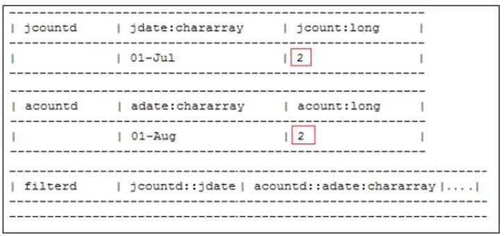
Output of illustrate
· ORDER BY: The ORDERBY operator is used to sort a relation using the sort key specified. As of today, Pig supports sorting on fields with simple types rather than complex types or expressions. In the following example, we are sorting based on two fields (July date and August date).
srtd = ORDER filterd BY jdate,adate PARALLEL 5;
· PARALLEL: The PARALLEL operator controls reduce-side parallelism by specifying the number of reducers. It is defaulted to one while running in a local mode. This clause can be used with operators, such as ORDER, DISTINCT, LIMIT, JOIN, GROUP, COGROUP, and CROSS that force a reduce phase.
· LIMIT: The LIMIT operator is used to set an upper limit on the number of output records generated. The output is determined randomly and there is no guarantee if the output will be the same if the LIMIT operator is executed consequently. To request a particular group of rows, you may consider using the ORDER operator, immediately followed by the LIMIT operator.
In our example, this operator returns five records as an illustration:
limitd = LIMIT srtd 5;
The content of the limitd tuple is given as follows:
(04-Jul,5806,04-Aug,4254)
(07-Jul,6951,07-Aug,4062)
(08-Jul,3064,08-Aug,4252)
(10-Jul,4383,10-Aug,4423)
(11-Jul,4819,11-Aug,4500)
· FLATTEN: The FLATTEN operator is used to make relations such as bags and tuple flat by removing the nesting in them. Please refer to the example code in DISTINCT for the sample output and usage of FLATTEN.
The EXPLAIN operator
A Pig program goes through multiple stages as shown in the next diagram, before being executed in the Hadoop cluster, and the EXPLAIN operator provides the best way to understand what transpires underneath the Pig Latin code. The EXPLAIN operator generates the sequence of plans that go into converting the Pig Latin scripts to a MapReduce JAR.
The output of this operator can be converted into a graphical format by the use of the -dot option to generate graphs of the program. This writes the output to a DOT file containing diagrams explaining the execution of our script.
The syntax for the same is as follows:
pig -x mapreduce -e 'pigexample.pig' -dot -out <filename> or <directoryname>
Next is an example of usage. If we specify a filename directory after -out, all the three output files (logical, physical, and MapReduce plan files) will get created in that directory. In the next case, all files will get created in the pigexample_output directory.
pig -x mapreduce -e ' pigexample.pig' -dot -out pigexample_output
Follow the given steps to convert the DOT files into an image format:
1. Install graphviz on your machine.
2. Plot a graph written in Dot language by executing the following command:
dot –Tpng filename.dot > filename.png
The following diagram shows each step in Pig processing:
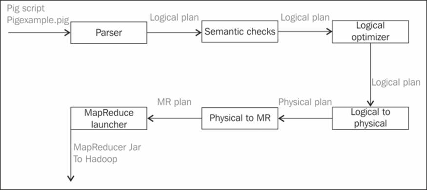
Pig Latin to Hadoop JAR
· The query parser: The parser uses ANother Tool for Language Recognition (ANTLR), a language parser, to verify whether the program is correct syntactically and if all the variables are properly defined. The parser also checks the schemas for type correctness and generates intermediate representation, Abstract Syntax Tree (AST).
· The logical plan: The intermediate representation, AST, is transformed into a logical plan. This plan is implemented internally as a directed graph with all the operators in the Pig Latin script mapped to the logical operators. The following diagram illustrates this plan:
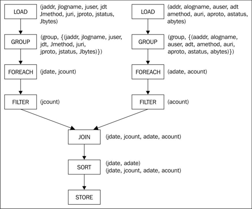
Logical plan
· The logical optimization: The logical plan generated is examined for opportunities of optimization such as filter-projection pushdown and column pruning. These are considered depending on the script. Optimization is performed and then the plan is compiled into a series of physical plans.
· The physical plan: The physical plan is a physical description of the computation that creates a usable pipeline, which is independent of MapReduce. We could use this pipeline and target other processing frameworks such as Dryad. The opportunities for optimizations in this stage are in memory aggregations instead of using combiners. The physical planning stage is also the right place where the plan is examined for the purpose of reducing the number of reducers.
For clarity, each logical operator is shown with an ID. Physical operators that are produced by the translation of a logical operator are shown with the same ID. For the most part, each logical operator becomes a corresponding physical operator. The logicalGROUP operator maps into a series of physical operators: local and global rearrange plus package. Rearrange is just like the Partitioner class and Reducer step of the MapReduce where sorting by a key happens.
The following diagram shows the logical plan translated to a physical plan example:
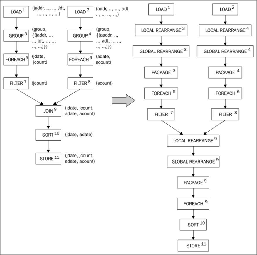
Logical to physical plan
· MapReduce plan: This is the phase where the physical plan is converted into a graph of actual MapReduce jobs with all the inputs and outputs specified. Opportunities for optimization in the MapReduce phase are examined to see if it is possible to combine multiple MapReduce jobs into one job for reducing the data flow between Mappers and Reducers. The idea of decoupling the Logical and Physical plans from the MapReduce plan is to divorce them from the details of running on Hadoop. This level of abstraction is necessary to port the application to a different processing framework like Dryad.
The following Physical to MapReduce Plan shows the assignment of the physical operators to Hadoop stages for our running example (only the map and reduce stages are shown). In the MapReduce plan, the local rearrange operator interprets tuples with keys and input stream's identifiers.
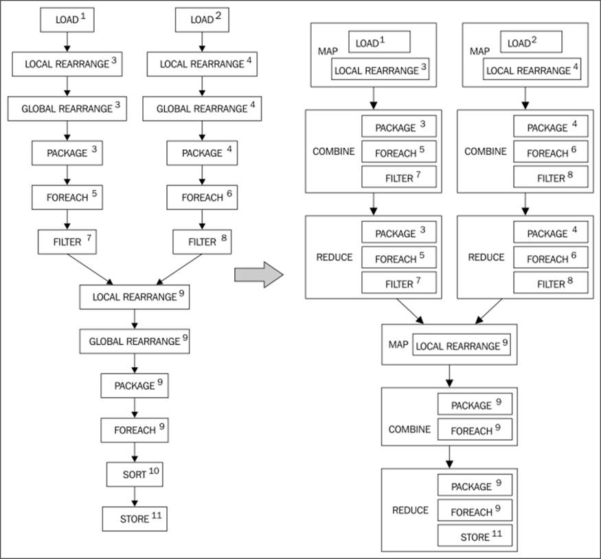
Physical to the MapReduce plan
Understanding Pig's data model
The Pig's data model consists of both primitive and complex types. The following sections give a brief overview of these data types:
Primitive types
Pig supports primitive data types such as Int, Float, Long, Double, and Chararray.
Complex types
The following are the complex data types, formed by combining the primitive data types:
· Atom: An atom contains a single value and can be composed of any one of the primitive data types.
· Tuple: A tuple is like a row of a table in an RDBMS, or a sequence of fields, each of which can be any of the data types including primitive and complex types. Tuples are enclosed in parentheses, (). An example is shown as follows:
(163.205.85.3,-,-,13/Jul/1995:08:51:12 -0400,GET,/htbin/cdt_main.pl,HTTP/1.0,200,3585)
· Bag: A bag is analogous to a table and a collection of tuples, which may have duplicates too. Bag is Pig's only spillable data structure, which implies that when the full structure does not fit in memory, it is spilled on to the disk and paged in when necessary. In a Bag, the schema of the constituent tuples is flexible and doesn't need to have a consistent number and type of fields. Bags are represented by data or tuple in curly braces, {}. An example is shown as follows:
· {(163.205.85.3,-,-,13/Jul/1995:08:51:12 -0400,GET,/htbin/cdt_main.pl,HTTP/1.0,200,3585)
(100.305.185.30,-,-,13/AUG/1995:09:51:12 -0400,GET,/htbin/cdt_main.pl,HTTP/1.0,200,3585)}
· Map: This is a key value data structure. The schema of the data items in a Map is not strictly enforced, giving the option to take the form of any type. Map is useful to prototype datasets where schemas may change over time. Maps are enclosed in square braces, [].
The relevance of schemas
Pig has a special way to handle known and unknown schemas. Schemas exist to give fields their identity by naming them and categorizing them into a data type. Pig has the ability to discover schemas at runtime by making appropriate assumptions about the data types. In case the data type is not assigned, Pig defaults the type to bytearray and performs conversions later, based on the context in which that data is used. This feature gives Pig an edge when you want to use it for research purposes to create quick prototypes on data with the unknown schema. Notwithstanding these advantages of working with unspecified schemas, it is recommended to specify the schema wherever or whenever it is possible for more efficient parse-time checking and execution. However, there are a few idiosyncrasies of how Pig handles unknown schemas when using various operators.
For the relational operators that perform JOIN, GROUP, UNION, or CROSS, if any one of the operators in the relation doesn't have a schema specified, then the resultant relation would be null. Similarly, a null would be the result when you try to flatten a bag with unknown schema.
Extending the discussion of how nulls can be resulted in Pig as in the preceding section, there are a few other ways nulls could result through the interaction of specific operators. As a quick illustration, if any of the subexpression operand in the comparison operators, such as ==, <, >, and MATCHES are null, then the result would be null. The same is applicable to arithmetic operators (such as +, -, *, /) and the CONCAT operators too. It is important to remember subtle differences between how various functions respect a null. While the AVG, MAX, MIN, SUM, and COUNT functions disregard nulls, the COUNT_STAR function does not ignore it and counts a null as if there is a value to it.
Summary
In this chapter, we have covered a wide array of ideas, with the central theme of keeping your focus latched on to Pig and then exploring its periphery. We understood what design patterns are and the way they are discovered and applied, from the perspective of Pig. We explored what Hadoop is, but we did it from a viewpoint of the historical enterprise context and figured out how Hadoop rewrote the history of distributed computing by addressing the challenges of the traditional architectures.
We understood how Pig brought in a fresh approach to programming Hadoop in an intuitive style, and we could comprehend the advantages it offers over other approaches of programming, plus it has given us the facility to write code in scripting-like language, which is easy to understand for those who already know scripting or don't want to code in Java MapReduce; with a small set of functions and operators, it provides us with the power to process an enormous amount of data quickly. We used a code example through which we understood the internals of Pig. The emphasis of this section was to cover as much ground as possible without venturing too deep into Pig and give you a ready reckoner to understand Pig.
In the next chapter, we will extend our understanding of the general concepts of using Pig in enterprises to specific use cases where Pig can be used for the input and output of data from a variety of sources. We shall begin by getting a ring-side view of all the data that gets into the enterprise and how it is consumed, and then we will branch out to look at a specific type of data more closely, and apply our patterns to it. These branches deal with unstructured, structured, and semi-structured data. Within each branch, we will learn how to apply patterns for each of the subbranches that deal with multiple aspects and attributes.
All materials on the site are licensed Creative Commons Attribution-Sharealike 3.0 Unported CC BY-SA 3.0 & GNU Free Documentation License (GFDL)
If you are the copyright holder of any material contained on our site and intend to remove it, please contact our site administrator for approval.
© 2016-2026 All site design rights belong to S.Y.A.