Pig Design Patterns (2014)

Chapter 6. Understanding Data Reduction Patterns

In the previous chapter, we learned about the various Big Data transformation techniques that dealt with transforming the structure of the data to a hierarchical representation. This was done in order to take advantage of Hadoop's capability to process semistructured data. We have seen the importance of performing normalization on the data before performing analysis on it. We then discussed using joins to denormalize the data. CUBE and ROLLUP perform multiple aggregations on the data; these aggregations provide a snapshot of the data. In the data generalization section, we discussed various generalization techniques for numerical and categorical data.

In this chapter, we will discuss design patterns that perform dimensionality reduction using the principal component analysis technique, and numerosity reduction using clustering, sampling, and histogram techniques.

Data reduction – a quick introduction

Data reduction aims to obtain a reduced representation of the data. It ensures data integrity, though the obtained dataset after the reduction is much smaller in volume than the original dataset.

Data reduction techniques are classified into the following three groups:

· Dimensionality reduction: This group of data reduction techniques deals with reducing the number of attributes that are considered for an analytics problem. They do this by detecting and eliminating the irrelevant attributes, relevant yet weak attributes, or redundant attributes. The principal component analysis and wavelet transforms are examples of dimensionality reduction techniques.

· Numerosity reduction: This group of data reduction techniques reduces the data by replacing the original dataset with a sparse representation of the data. The sparse subset of the data is computed by parametric methods such as regression, where a model is used to estimate the data so that only a subset is enough instead of the entire dataset. There are other methods such as nonparametric methods, for example, clustering, sampling, and histograms, which work without the need for a model to be built.

· Compression: This group of data reduction techniques uses algorithms to reduce the size of the physical storage that the data consumes. Typically, compression is performed at a higher level of granularity than at the attribute or record level. If you need to retrieve the original data from the compressed data without any loss of information, which is required while storing string or numerical data, a lossless compression scheme is used. If instead, there is a need to uncompress video and sound files that can accommodate the imperceptible loss of clarity, then lossy compression techniques are used.

The following diagram illustrates the different techniques that are used in each of the aforementioned groups:

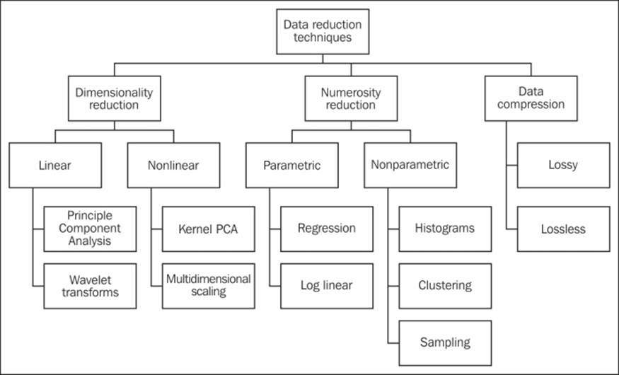
Data reduction – a quick introduction

Data reduction techniques – overview

Data reduction considerations for Big Data

In Big Data problems, data reduction techniques have to be considered as part of the analytics process rather than a separate process. This will enable you to understand what type of data has to be retained or eliminated due to its irrelevance to the analytics-related questions that are asked.

In a typical Big Data analytical environment, data is often acquired and integrated from multiple sources. Even though there is the promise of a hidden reward for using the entire dataset for the analytics, which in all probability may yield richer and better insights, the cost of doing so sometimes overweighs the results. It is at this juncture that you may have to consider reducing the amount of data without drastically compromising on the effectiveness of the analytical insights, in essence, safeguarding the integrity of the data.

Performing any type of analysis on Big Data often leads to high storage and retrieval costs owing to the massive amount of data. The benefits of data reduction processes are sometimes not evident when the data is small; they begin to become obvious when the datasets start growing in size. These data reduction processes are one of the first steps that are taken to optimize data from the storage and retrieval perspective. It is important to consider the ramifications of data reduction so that the computational time spent on it does not outweigh or erase the time saved by data mining on a reduced dataset size. Now that we have understood data reduction concepts, we will explore a few concrete design patterns in the following sections.

Dimensionality reduction – the Principal Component Analysis design pattern

In this design pattern, we will consider one way of implementing the dimensionality reduction through the usage of Principal Component Analysis (PCA) and Singular value decomposition (SVD), which are versatile techniques that are widely used for exploratory data analysis, creating predictive models, and for dimensionality reduction.

Background

Dimensions in a given data can be intuitively understood as a set of all attributes that are used to account for the observed properties of data. Reducing the dimensionality implies the transformation of a high dimensional data into a reduced dimension's set that is proportional to the intrinsic or latent dimensions of the data. These latent dimensions are the minimum number of attributes that are needed to describe the dataset. Thus, dimensionality reduction is a method to understand the hidden structure of data that is used to mitigate the curse of high dimensionality and other unwanted properties of high dimensional spaces.

Broadly, there are two ways to perform dimensionality reduction. One of them is the linear dimensionality reduction, examples of which are PCA and SVD. The other is the nonlinear dimensionality reduction for which kernel PCA and Multidimensional Scaling are the examples.

In this design pattern, we explore linear dimensionality reduction by implementing PCA in R and SVD in Mahout and integrating them with Pig.

Motivation

Let's first have an overview of PCA. PCA is a linear dimensionality reduction technique that works unsupervised on a given dataset by implanting the dataset into a subspace of lower dimensions, which is done by constructing a variance-based representation of the original data.

The underlying principle of PCA is to identify the hidden structure of the data by analyzing the direction where the variation of data is the most or where the data is most spread out.

Intuitively, a principal component can be considered as a line, which passes through a set of data points that vary to a greater degree. If you pass the same line through data points with no variance, it implies that the data is the same and does not carry much information. In cases where there is no variance, data points are not considered as representatives of the properties of the entire dataset, and these attributes can be omitted.

PCA involves finding pairs of eigenvalues and eigenvectors for a dataset. A given dataset is decomposed into pairs of eigenvectors and eigenvalues. An eigenvector defines the unit vector or the direction of the data perpendicular to the others. An eigenvalue is the value of how spread out the data is in that direction.

In multidimensional data, the number of eigenvalues and eigenvectors that can exist are equal to the dimensions of the data. An eigenvector with the biggest eigenvalue is the principal component.

After finding out the principal component, they are sorted in the decreasing order of eigenvalues so that the first vector shows the highest variance, the second shows the next highest, and so on. This information helps uncover the hidden patterns that were not previously suspected and thereby allows interpretations that would not result ordinarily.

As the data is now sorted in the decreasing order of significance, the data size can be reduced by eliminating the attributes with a weak component, or low significance where the variance of data is less. Using the highly valued principal components, the original dataset can be constructed with a good approximation.

As an example, consider a sample election survey conducted on a hundred million people who have been asked 150 questions about their opinions on issues related to elections. Analyzing a hundred million answers over 150 attributes is a tedious task. We have a high dimensional space of 150 dimensions, resulting in 150 eigenvalues/vectors from this space. We order the eigenvalues in descending order of significance (for example, 230, 160, 130, 97, 62, 8, 6, 4, 2,1… up to 150 dimensions). As we can decipher from these values, there can be 150 dimensions, but only the top five dimensions possess the data that is varying considerably. Using this, we were able to reduce a high dimensional space of 150 and could consider the top five eigenvalues for the next step in the analytics process.

Next, let's look into SVD. SVD is closely related to PCA, and sometimes both terms are used as SVD, which is a more general method of implementing PCA. SVD is a form of matrix analysis that produces a low-dimensional representation of a high-dimensional matrix. It achieves data reduction by removing linearly dependent data. Just like PCA, SVD also uses eigenvalues to reduce the dimensionality by combining information from several correlated vectors to form basis vectors that are orthogonal and explains most of the variance in the data.

For example, if you have two attributes, one is sale of ice creams and the other is temperature, then their correlation is so high that the second attribute, temperature, does not contribute any extra information useful for a classification task. The eigenvalues derived from SVD determines which attributes are most informative and which ones you can do without.

Mahout's Stochastic SVD (SSVD) is based on computing mathematical SVD in a distributed fashion. SSVD runs in the PCA mode if the pca argument is set to true; the algorithm computes the column-wise mean over the input and then uses it to compute the PCA space.

Use cases

You can consider using this pattern to perform data reduction, data exploration, and as an input to clustering and multiple regression.

The design pattern can be applied on ordered and unordered attributes with sparse and skewed data. It can also be used on images. This design pattern cannot be applied on complex nonlinear data.

Pattern implementation

The following steps describe the implementation of PCA using R:

· The script applies the PCA technique to reduce dimensions. PCA involves finding pairs of eigenvalues and eigenvectors for a dataset. An eigenvector with the biggest eigenvalue is the principal component. The components are sorted in the decreasing order of eigenvalues.

· The script loads the data and uses streaming to call the R script. The R script performs PCA on the data and returns the principal components. Only the first few principal components that can explain most of the variation can be selected so that the dimensionality of the data is reduced.

Limitations of PCA implementation

While streaming allows you to call the executable of your choice, it has performance implications, and the solution is not scalable in situations where your input dataset is huge. To overcome this, we have shown a better way of performing dimensionality reduction by using Mahout; it contains a set of highly scalable machine learning libraries.

The following steps describe the implementation of SSVD on Mahout:

· Read the input dataset in the CSV format and prepare a set of data points in the form of key/value pairs; the key should be unique and the value should comprise of n vector tuples.

· Write the previous data into a sequence file. The key can be of a type adapted into WritableComparable, Long, or String, and the value should be of the VectorWritable type.

· Decide on the number of dimensions in the reduced space.

· Execute SSVD on Mahout with the rank arguments (this specifies the number of dimensions), setting pca, us, and V to true. When the pca argument is set to true, the algorithm runs in the PCA mode by computing the column-wise mean over the input and then uses it to compute the PCA space. The USigma folder contains the output with reduced dimensions.

Generally, dimensionality reduction is applied on very high dimensional datasets; however, in our example, we have demonstrated this on a dataset with fewer dimensions for a better explainability.

Code snippets

To illustrate the working of this pattern, we have considered the retail transactions dataset that is stored on the Hadoop File System (HDFS). It contains 20 attributes, such as Transaction ID, Transaction date, Customer ID, Product subclass, Phone No, Product ID, age,quantity, asset, Transaction Amount, Service Rating, Product Rating, and Current Stock. For this pattern, we will be using PCA to reduce the dimensions. The following code snippet is the Pig script that illustrates the implementation of this pattern via Pig streaming:

Assign an alias pcar to the streaming command

Use ship to send streaming binary files (R script in this use case) from the client node to the compute node

DEFINE pcar '/home/cloudera/pdp/data_reduction/compute_pca.R' ship('/home/cloudera/pdp/data_reduction/compute_pca.R');

Load the data set into the relation transactions

transactions = LOAD '/user/cloudera/pdp/datasets/data_reduction/transactions_multi_dims.csv' USING PigStorage(',') AS (transaction_id:long, transaction_date:chararray, customer_id:chararray, prod_subclass:chararray, phone_no:chararray, country_code:chararray, area:chararray, product_id:chararray, age:int, amt:int, asset:int, transaction_amount:double, service_rating:int, product_rating:int, curr_stock:int, payment_mode:int, reward_points:int, distance_to_store:int, prod_bin_age:int, cust_height:int);

Extract the columns on which PCA has to be performed.

STREAM is used to send the data to the external script.

The result is stored in the relation princ_components

selected_cols = FOREACH transactions GENERATE age AS age, amt AS amount, asset AS asset, transaction_amount AS transaction_amount, service_rating AS service_rating, product_rating AS product_rating, curr_stock AS current_stock, payment_mode AS payment_mode, reward_points AS reward_points, distance_to_store AS distance_to_store, prod_bin_age AS prod_bin_age, cust_height AS cust_height;

princ_components = STREAM selected_cols THROUGH pcar;

The results are stored on the HDFS in the directory pca

STORE princ_components INTO '/user/cloudera/pdp/output/data_reduction/pca';

Following is the R code illustrating the implementation of this pattern:

#! /usr/bin/env Rscript

options(warn=-1)

#Establish connection to stdin for reading the data

con <- file("stdin","r")

#Read the data as a data frame

data <- read.table(con, header=FALSE, col.names=c("age", "amt", "asset", "transaction_amount", "service_rating", "product_rating", "current_stock", "payment_mode", "reward_points", "distance_to_store", "prod_bin_age", "cust_height"))

attach(data)

#Calculate covariance and correlation to understand the variation between the independent variables

covariance=cov(data, method=c("pearson"))

correlation=cor(data, method=c("pearson"))

#Calculate the principal components

pcdat=princomp(data)

summary(pcdat)

pcadata=prcomp(data, scale = TRUE)

pcadata

The ensuing code snippets illustrate the implementation of this pattern using Mahout's SSVD. The following is a snippet of a shell script with the commands for executing CSV to the sequence converter:

#All the mahout jars have to be included in HADOOP_CLASSPATH before execution of this script.

#Execute csvtosequenceconverter jar to convert the CSV file to sequence file.

hadoop jar csvtosequenceconverter.jar com.datareduction.CsvToSequenceConverter /user/cloudera/pdp/datasets/data_reduction/transactions_multi_dims_ssvd.csv /user/cloudera/pdp/output/data_reduction/ssvd/transactions.seq

The following is the code snippet of the Pig script with commands for executing SSVD on Mahout:

*Ideally the following data pre-processing steps have to be generally performed on the actual data, we have deliberately omitted the implementation as these steps were covered in the respective chapters

*Data Ingestion to ingest data from the required sources

*Data Profiling by applying statistical techniques to profile data and find data quality issues

*Data Validation to validate the correctness of the data and cleanse it accordingly

*Data Transformation to apply transformations on the data.

Use sh command to execute shell commands.

Convert the files in a directory to sequence files

-i specifies the input path of the sequence file on HDFS

-o specifies the output directory on HDFS

-k specifies the rank, i.e the number of dimensions in the reduced space

-us set to true computes the product USigma

-V set to true computes V matrix

-pca set to true runs SSVD in pca mode

sh /home/cloudera/mahout-distribution-0.8/bin/mahout ssvd -i /user/cloudera/pdp/output/data_reduction/ssvd/transactions.seq -o /user/cloudera/pdp/output/data_reduction/ssvd/reduced_dimensions -k 7 -us true -V true -U false -pca true -ow -t 1

Use seqdumper to dump the output in text format.

-i specifies the HDFS path of the input file

sh /home/cloudera/mahout-distribution-0.8/bin/mahout seqdumper -i /user/cloudera/pdp/output/data_reduction/ssvd/reduced_dimensions/V/v-m-00000

Results

The following is a snippet of the result of executing the R script through Pig streaming. Only the important components in the results are shown to improve readability.

Importance of components:

Comp.1 Comp.2 Comp.3

Standard deviation 1415.7219657 548.8220571 463.15903326

Proportion of Variance 0.7895595 0.1186566 0.08450632

Cumulative Proportion 0.7895595 0.9082161 0.99272241

The following diagram shows a graphical representation of the results:

Results

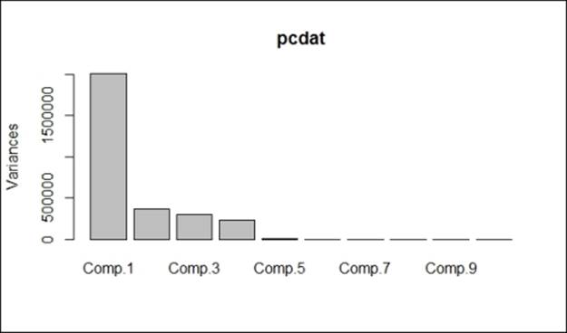
PCA output

From the cumulative results, we can explain most of the variation with the first three components. Hence, we can drop the other components and still explain most of the data, thereby achieving data reduction.

The following is a code snippet of the result attained after applying SSVD on Mahout:

Key: 0: Value: {0:6.78114976729216E-5,1:-2.1865954292525495E-4,2:-3.857078959222571E-5,3:9.172780131217343E-4,4:-0.0011674781643860148,5:-0.5403803571549012,6:0.38822546035077155}

Key: 1: Value: {0:4.514870142377153E-6,1:-1.2753047299542729E-5,2:0.002010945408634006,3:2.6983823401328314E-5,4:-9.598021198119562E-5,5:-0.015661212194480658,6:-0.00577713052974214}

Key: 2: Value: {0:0.0013835831436886054,1:3.643672803676861E-4,2:0.9999962672043754,3:-8.597640675661196E-4,4:-7.575051881399296E-4,5:2.058878196540628E-4,6:1.5620427291943194E-5}

Key: 11: Value: {0:5.861358116239576E-4,1:-0.001589570485260711,2:-2.451436184622473E-4,3:0.007553283166922416,4:-0.011038688645296836,5:0.822710349440101,6:0.060441819443160294}

The contents of the V folder show the contribution of the original variables to every principal component. The result is a 12 x 7 matrix as we have 12 dimensions in our original dataset, which were reduced to 7, as specified in the rank argument to SSVD.

The USigma folder contains the output with reduced dimensions.

Additional information

The complete code and datasets for this section are in the following GitHub directories:

· Chapter6/code/

· Chapter6/datasets/

Information on Mahout's implementation of SSVD can be found at the following links:

· https://cwiki.apache.org/confluence/display/MAHOUT/Stochastic+Singular+Value+Decomposition

· https://cwiki.apache.org/confluence/download/attachments/27832158/SSVD-CLI.pdf?version=18&modificationDate=1381347063000&api=v2

· http://en.wikibooks.org/wiki/Data_Mining_Algorithms_In_R/Dimensionality_Reduction/Singular_Value_Decomposition

Numerosity reduction – the histogram design pattern

The Numerosity reduction – histogram design pattern explores the implementation of the histograms technique for data reduction.

Background

Histograms belong to the numerosity reduction category of data reduction. They are nonparametric methods of data reduction in which it is assumed that the data does not fit into a predefined model or function.

Motivation

Histograms work by dividing the entire data into buckets or groups and storing the central tendency for each of the buckets. Internally, this resembles binning. Histograms can be constructed optimally using dynamic programming. Histograms differ from bar charts in that they represent continuous data categories rather than discrete categories. This implies that in a histogram, there are no gaps among columns that represent various categories.

Histograms help in reducing the categories of data by grouping a large number of continuous attributes. Representing a large number of attributes may result in a complex histogram with so many columns that it becomes difficult to interpret the information. Hence, the data is grouped into ranges that denote a continuous range of values for an attribute. The data can be grouped in the following ways:

· Equal-width grouping technique: In this grouping technique, each range is of uniform width.

· Equal-frequency (or equi-depth) grouping technique: In an equal-frequency grouping technique, the ranges are created in a way that either the frequency of each range is constant or each range contains the same number of contiguous data elements.

· V-Optimal grouping technique: In this grouping technique, we consider all the possible histograms for a given number of ranges and choose the one with the minimal variance.

· MaxDiff grouping technique: This histogram grouping technique considers grouping values into a range based on the difference between each pair of adjacent values. The range boundary is defined between each pair of adjacent points with the largest differences. The following diagram depicts sorted data that is grouped into three ranges identified by the maximum differences between 9-14 and 18-27.

Motivation

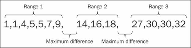
Maximum difference – illustration

In the previously mentioned grouping techniques, the V-Optimal and MaxDiff techniques are more accurate and effective for approximating both sparse and dense data, as well as highly skewed and uniform data. These histograms can also work on multiple attributes by using multidimensional histograms that can capture dependencies between attributes.

Use cases

You can consider using this design pattern in the following conditions:

· When the data does not fit into a parametric model such as regression or log-linear models

· When the data is continuous and not discrete

· When the data has ordered or unordered numeric attributes

· When the data is skewed or sparse

Pattern implementation

The script loads the data and divides it into buckets using equal-width grouping. The data for the Transaction Amount field is grouped into buckets. It counts the number of transactions in each bucket and returns the bucket range and the count as the output.

This pattern produces a reduced representation of the dataset where the transaction amount is divided into the specified number of buckets and the count of transactions that fall in that range. This data is plotted as a histogram.

Code snippets

To illustrate the working of this pattern, we have considered the retail transactions dataset stored on the HDFS. It contains attributes such as Transaction ID, Transaction date, Customer ID, age, Phone Number, Product, Product subclass, Product ID, Transaction Amount, andCountry Code. For this pattern, we will be generating buckets on the attribute Transaction Amount. The following code snippet is the Pig script illustrating the implementation of this pattern:

Define the alias generateBuckets for the custom UDF, the number of buckets(20) is passed as a parameter

DEFINE generateBuckets com.datareduction.GenerateBuckets('20');

Load the dataset into the relation transactions

transactions = LOAD '/user/cloudera/pdp/datasets/data_reduction/transactions.csv' USING PigStorage(',') AS (transaction_id:long,transaction_date:chararray, cust_id:chararray, age:chararray, area:chararray, prod_subclass:int, prod_id:long, quantity:int, asset:int, transaction_amt:double, phone_no:chararray, country_code:chararray);

Maximum value of transactions amount and the actual transaction amount are passed to generateBuckets UDF

The UDF calculates the bucket size by dividing maximum transaction amount by the number of buckets.

It finds out the range to which each value belongs to and returns the value along with the bucket range

transaction_amt_grpd = GROUP transactions ALL;

transaction_amt_min_max = FOREACH transaction_amt_grpd GENERATE MAX(transactions.transaction_amt) AS max_transaction_amt,FLATTEN(transactions.transaction_amt) AS transaction_amt;

transaction_amt_buckets = FOREACH transaction_amt_min_max GENERATE generateBuckets(max_transaction_amt,transaction_amt) ;

Calculate the count of values in each range

transaction_amt_buckets_grpd = GROUP transaction_amt_buckets BY range;

transaction_amt_buckets_count = FOREACH transaction_amt_buckets_grpd GENERATE group, COUNT(transaction_amt_buckets);

The results are stored on HDFS in the directory histogram.

STORE transaction_amt_buckets_count INTO '/user/cloudera/pdp/output/data_reduction/histogram';

The following code snippet is the Java UDF code that illustrates the implementation of this pattern:

@Override

public String exec(Tuple input) throws IOException {

if (input == null || input.size() ==0)

return null;

try{

//Extract the maximum transaction amount

max = Double.parseDouble(input.get(0).toString());

//Extract the value

double rangeval = Double.parseDouble(input.get(1).toString());

/*Calculate the bucket size by dividing maximum

transaction amount by the number of buckets.

setBucketSize();

/*Set the bucket range by using the bucketSize and

noOfBuckets

setBucketRange();

It finds out the range to which each value belongs

to and returns the value along with the bucket range

return getBucketRange(rangeval);

} catch(Exception e){

System.err.println("Failed to process input; error - " + e.getMessage());

return null;

}

Results

The following is a snippet of the result of applying this pattern on the dataset; the first column is the bucket range of the Transaction Amount attribute and the second column is the count of transactions:

1-110 45795

110-220 50083

220-330 60440

330-440 40001

440-550 52802

The following is the histogram generated by plotting this data using gnuplot. It shows a graphical representation of the transaction amount buckets and the number of transactions in each bucket.

Results

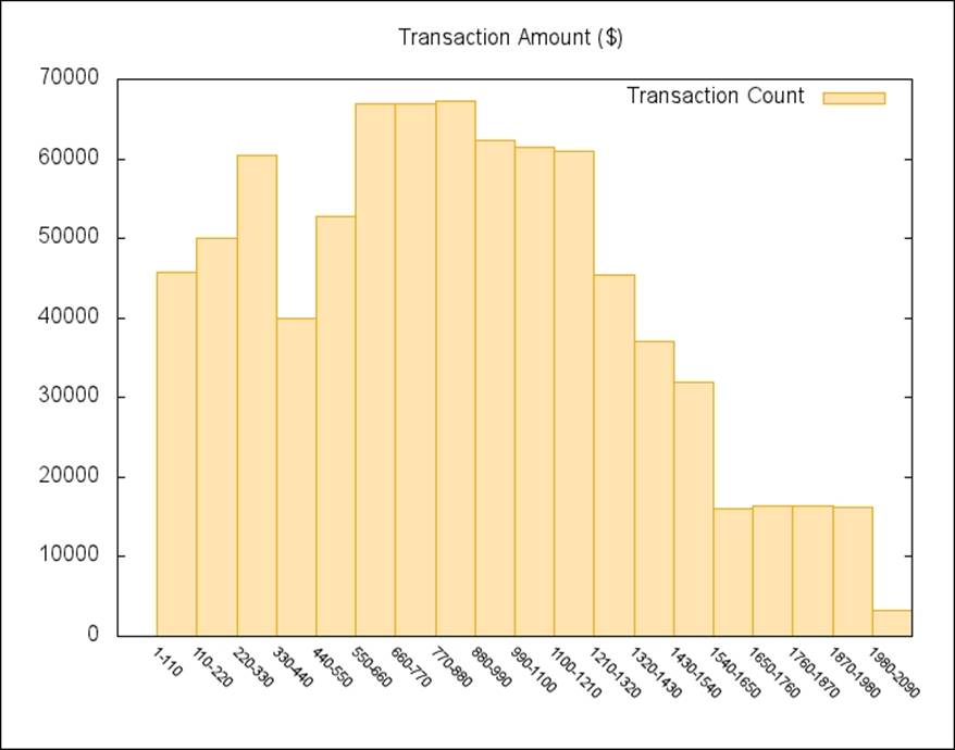
Histogram output

Additional information

The complete code and datasets for this section are in the following GitHub directories:

· Chapter6/code/

· Chapter6/datasets/

Numerosity reduction – sampling design pattern

This design pattern explores the implementation of sampling techniques for data reduction.

Background

Sampling belongs to the numerosity reduction category of data reduction. It can be used as a data reduction technique, as it represents a very large amount of data by a much smaller subset.

Motivation

Sampling is essentially a method of data reduction to determine the approximate subset of a population that has the characteristics of the entire population. Sampling is a general approach to choose a subset of data to accurately represent a population. Sampling is performed by various methods that differ in the way in which they define what goes into the subset and the way candidates are located for that subset.

In the Big Data scenario, the cost of performing analytics, such as classification and optimization, over the complete population is high; sampling helps to reduce the cost by reducing the footprint of the data used to perform the actual analytics and then extrapolating the results on the population. There would be marginal loss of accuracy, but it far outweighs the benefits of reduced time versus storage trade-offs.

When it comes to Big Data, wherever techniques of statistical sampling are applied, it is important to be cognizant of the population about which one aims to perform the analytics. Even if the data that has been collected is very big, the samples may relate only to a small part of the population, and they may not represent the whole. While picking the sample, representativeness plays a vital role, as it determines how close the sampled data is to the population.

Sampling can be performed using probabilistic and nonprobabilistic methods. The following diagram captures the broad landscape of the techniques involved in sampling:

Motivation

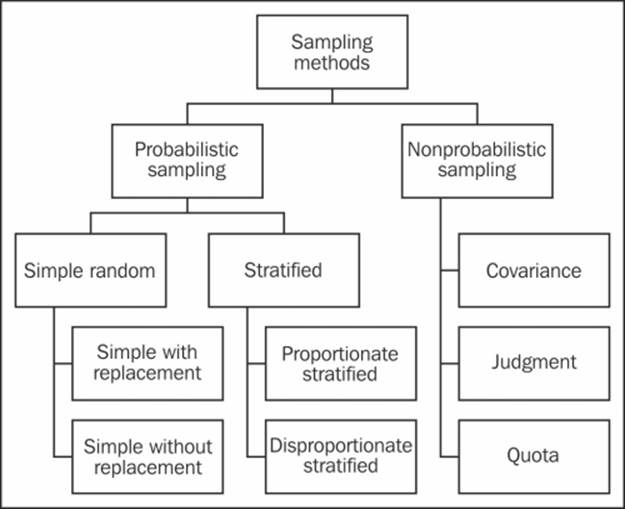
Sampling methods

Probabilistic sampling methods use random sampling, and every element in the population has a known nonzero (greater than zero) chance of getting selected into the sampled subset. Probabilistic sampling methods use weighted sampling and result in unbiased samples of the population. The following are a few probabilistic sampling methods:

· Simple random sampling: This is the most basic type of sampling in which every element of the population has an equal chance of being selected into the subset. The samples are objectively selected at random. The simple random sampling can be done by replacing the selected item in the population so that it can be selected again (sampling with replacement) or by not replacing the selected item in the population (sampling without replacement). Random sampling doesn't always result in a representative sample and is a costly operation to perform on a very large dataset. The representativeness of random sampling can be improved by presampling the population using stratification or clustering.

· The following diagram illustrates the difference between the Simple Random Sampling Without Replacement (SRSWOR) and Simple Random Sampling With Replacement (SRSWR).

Motivation

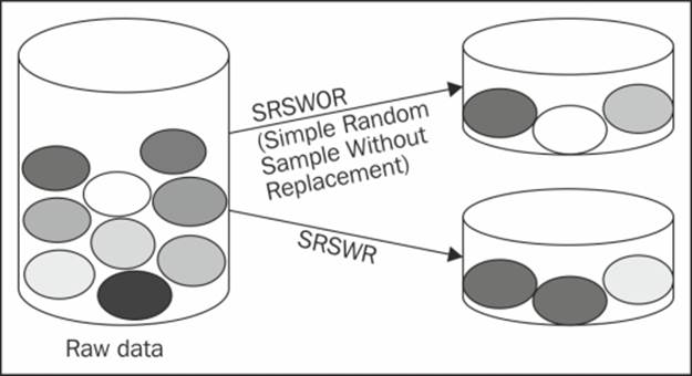
SRSWOR versus SRSWR

· Stratified sampling: This sampling technique is used when we already know that the population contains a number of unique categories that are used to organize the population into subpopulations (strata); individual samples can then be picked out of them. The chosen sample is forced to contain elements from each of the subpopulations. This sampling method concentrates on relevant subpopulations and ignores the irrelevant ones. The representativeness of the sample is increased by eliminating the selection by absolute randomness, as evidenced in the simple random sampling and by selecting items from the independent strata. The stratified sampling method is a more efficient sampling technique in cases where the unique categories of the strata are identified in advance. There is an overall time-cost trade-off associated with stratified sampling, as it could be tedious to initially identify the unique categories for a population that is relatively homogeneous.

· NonProbabilistic sampling: This sampling method selects the subset of the population without giving an equal chance of selection to some elements of the population. In this sampling, the probability of the selection of the elements cannot be accurately determined. The selection of the elements is done purely based on a few assumptions on the population of interest. Nonprobabilistic sampling score poorly to accurately represent the population, and hence the resultant analytics cannot be extrapolated from the sample to the population. Nonprobabilistic sampling methods include the covariance sampling, the judgment sampling, and the quota sampling methods.

Use cases

You can consider using the numerosity reduction sampling design pattern in the following scenarios:

· When the data is continuous or discrete

· When each element of the data has an equal chance of getting selected without affecting the representativeness of the sampling

· When the data has ordered or unordered attributes

Pattern implementation

This design pattern is implemented in Pig as a standalone script. It uses the datafu library, which has the implementation of SRSWR as a pair of UDFs, SimpleRandomSampleWithReplacementElect and SimpleRandomSampleWithReplacementVote; they implement a scalable algorithm for SRSWR. The algorithm consists of two phases: vote and elect. Candidates for each position are voted during the vote stage. One candidate per position is elected during the election stage. The output is a bag of sampled data.

The script selects a sample of 100,000 records from the transactions dataset using the SRSWR technique.

Code snippets

To illustrate the working of this pattern, we have considered the retail transactions dataset stored on the HDFS. It contains attributes such as Transaction ID, Transaction date, Customer ID, age, Phone Number, Product, Product subclass, Product ID, Transaction Amount, andCountry Code. For this pattern, we will be performing SRSWR on the transactions dataset. The following code snippet is the Pig script that illustrates the implementation of this pattern:

Define aliases for the classes SimpleRandomSampleWithReplacementVote and SimpleRandomSampleWithReplacementElect

DEFINE SRSWR_VOTE datafu.pig.sampling.SimpleRandomSampleWithReplacementVote();

DEFINE SRSWR_ELECT datafu.pig.sampling.SimpleRandomSampleWithReplacementElect();

Load the dataset into the relation transactions

transactions= LOAD '/user/cloudera/pdp/datasets/data_reduction/transactions.csv' USING PigStorage(',') AS (transaction_id:long,transaction_date:chararray, cust_id:chararray, age:int, area:chararray, prod_subclass:int, prod_id:long, quantity:int, asset:int, transaction_amt:double, phone_no:chararray, country_code:chararray);

The input to Vote UDF is the bag of items, the desired sample size (100000 in our use case) and the actual population size.

This UDF votes candidates for each position

summary = FOREACH (GROUP transactions ALL) GENERATE COUNT(transactions) AS count;

candidates = FOREACH transactions GENERATE FLATTEN(SRSWR_VOTE(TOBAG(TOTUPLE(*)), 100000, summary.count));

The Elect UDF elects one candidate for each position and returns a bag of sampled items stored in the relation sampled

sampled = FOREACH (GROUP candidates BY position PARALLEL 10) GENERATE FLATTEN(SRSWR_ELECT(candidates));

The results are stored on the HDFS in the directory sampling

STORE sampled into '/user/cloudera/pdp/output/data_reduction/sampling';

Results

The following is a snippet of the results obtained after applying sampling on the transactions data. We have eliminated a few columns to improve readability.

580493 … 1621624 … … … … 1 115 576 900-435-5791 U.S.A

193016 … 1808643 … … … … 1 119 735 9020138550 U.S.A

800748 … 199995 … … … … 1 28 1577 904-066-467q USA

The result is a file that contains 100,000 records, taken as a sample from the original dataset.

Additional information

The complete code and datasets for this section are in the following GitHub directories:

· Chapter6/code/

· Chapter6/datasets/

Numerosity reduction – clustering design pattern

This design pattern explores the implementation of the clustering technique for data reduction.

Background

Clustering belongs to the numerosity reduction category of data reduction. Clustering is a nonparametric model and works without the prior knowledge of a class label using unsupervised learning.

Motivation

Clustering is a general approach to solve the problem of grouping data. It can be achieved by various algorithms that differ in the way they define what goes into a group and how to find the candidates for that group. There are more than 100 different implementations of clustering algorithms that solve a variety of problems for different objectives. There is no single size that fits all the clustering algorithms for a given problem; the appropriate one has to be chosen by careful experimentation. A clustering algorithm that works on a specific data model doesn't always work on a different model. Clustering is widely used in machine learning, image analysis, pattern recognition, and information retrieval.

The objective of clustering is to partition the dataset and effectively reduce its size based on a set of heuristics. Clustering is, in a way, similar to binning, since it mimics the grouping aspect of binning; however, the difference lies in the precise way the grouping is performed in clustering.

The partitions are performed in a way that the data in one cluster is similar to another in the same cluster, but is dissimilar to other data in other clusters. Here, similarity is defined as a measure of how close the data is to each other.

K Means is one of the most widely used methods for clustering. Partitions of observations into k clusters is done by K Means of the cluster analysis; here, each observation belongs to the cluster with the nearest mean. It is an iterative process and stabilizes only if the cluster centroid does not move any further.

The quality measure of how well the clustering was performed can be ascertained by measuring the diameter or the average distance of each cluster object from the cluster centroid.

We can intuitively understand the need for clustering to reduce the numerosity of data by the example of an apparel company planning to release a new model of t-shirt into the market. If the company doesn't use a data reduction technique, it ends up manufacturing t-shirts of varying sizes to cater to different people. In order to prevent this, they reduce the data by first noting down the height and weight of people, plotting them on a graph, and dividing them into three major clusters: small, medium, and large.

The K Means method uses the dataset of height and weight (n observations) and divides them into k (that is, three) clusters. For each of the cluster (small, medium, and large), the data points inside the cluster are closer to the cluster category (that is, mean of small's height and weight). K Means has provided us with the best three sizes that will fit everyone and has thus effectively reduced the complexity of the data; instead of working on the actual data, clustering enables us to work on the replacement of the actual data by clusters themselves.

Note

We have considered using the K Means implementation of Mahout; more information on this can be obtained from https://mahout.apache.org/users/clustering/k-means-clustering.html.

From a Big Data perspective, as there is a need to process a very large amount of data, there would be a time-quality trade-off to be taken into consideration for choosing a clustering algorithm. New research is underway to develop preclustering methods, which can process Big Data efficiently. However, the results of a preclustering method are an approximate prepartitioning of the original dataset, which will eventually be clustered again by traditional methods such as K Means.

Use cases

You can consider using this design pattern in the following cases:

· When the data is continuous or discrete and the class labels of the data are not known in advance

· When there is a need to preprocess the data by clustering for, eventually, performing the classification on a very large amount of data

· When the data has numeric, ordered, or unordered attributes

· When the data is categorical

· When the data is not skewed, sparsed, or smeared

Pattern implementation

The design pattern is implemented in Pig and Mahout. The dataset is loaded into Pig. The age attribute on which K Means clustering is to be performed is transformed into vectors and is stored into a Mahout-readable format. It applies Mahout's K Means clustering on the age attribute of the transactions dataset. K Means clustering partitions the observations into k clusters in which each observation belongs to the cluster with the nearest mean; the process is iterative and stabilizes only if the cluster centroid does not move any further.

This pattern produces a reduced representation of the dataset where the age attribute is partitioned into a predefined number of clusters. This information can be used to identify the age groups of the customers visiting the store.

Code snippets

To illustrate the working of this pattern, we have considered the retail transactions dataset stored on the HDFS. It contains attributes such as Transaction ID, Transaction date, Customer ID, age, Phone Number, Product, Product subclass, Product ID, Transaction Amount, andCountry Code. For this pattern, we will be performing K Means clustering on the age attribute. The following code snippet is the Pig script that illustrates the implementation of this pattern:

Use declare to create aliases.

declare is a preprocessor statement and is processed before running the script

%declare SEQFILE_LOADER 'com.twitter.elephantbird.pig.load.SequenceFileLoader';

%declare SEQFILE_STORAGE 'com.twitter.elephantbird.pig.store.SequenceFileStorage';

%declare VECTOR_CONVERTER 'com.twitter.elephantbird.pig.mahout.VectorWritableConverter';

%declare TEXT_CONVERTER 'com.twitter.elephantbird.pig.util.TextConverter';

Load the dataset into the relation transactions

transactions = LOAD '/user/cloudera/pdp/datasets/data_reduction/transactions.csv' USING PigStorage(',') AS (id:long,transaction_date:chararray, cust_id:int, age:int, area:chararray, prod_subclass:int, prod_id:long, quantity:int, asset:int, transaction_amt:double, phone_no:chararray, country_code:chararray);

Extract the columns on which clustering has to be performed

age = FOREACH transactions GENERATE id AS tid, 1 AS index, age AS cust_age;

Generate tuples from the parameters

grpd = GROUP age BY tid;

vector_input = FOREACH grpd generate group, org.apache.pig.piggybank.evaluation.util.ToTuple(age.(index, cust_age));

Use elephant bird functions to store the data into sequence file (mahout readable format)

cardinality represents the dimension of the vector.

STORE vector_input INTO '/user/cloudera/pdp/output/data_reduction/kmeans_preproc' USING $SEQFILE_STORAGE (

'-c $TEXT_CONVERTER', '-c $VECTOR_CONVERTER -- -cardinality 100'

);

The following is a snippet of a shell script with the commands for executing K Means clustering on Mahout:

#All the mahout jars have to be included in classpath before execution of this script.

#Create the output directory on HDFS before executing VectorConverter

hadoop fs -mkdir /user/cloudera/pdp/output/data_reduction/kmeans_preproc_nv

#Execute vectorconverter jar to convert the input to named vectors

hadoop jar /home/cloudera/pdp/data_reduction/vectorconverter.jar com.datareduction.VectorConverter /user/cloudera/pdp/output/data_reduction/kmeans_preproc/ /user/cloudera/pdp/output/data_reduction/kmeans_preproc_nv/

#The below Mahout command shows the usage of kmeans. The algorithm takes the input vectors from the path specified in the -i argument, it chooses the initial clusters at random, -k argument specifies the number of clusters as 3, -x specified the maximum number of iterations as 15. -dm specifies the distance measure to use i.e euclidean distance and a convergence threshold specified in -cd as 0.1

/home/cloudera/mahout-distribution-0.7/bin/mahout kmeans -i /user/cloudera/pdp/output/data_reduction/kmeans_preproc_nv/ -c kmeans-initial-clusters -k 3 -o /user/cloudera/pdp/output/data_reduction/kmeans_clusters -x 15 -ow -cl -dm org.apache.mahout.common.distance.EuclideanDistanceMeasure -cd 0.01

# Execute cluster dump command to print information about the cluster

/home/cloudera/mahout-distribution-0.7/bin/mahout clusterdump --input /user/cloudera/pdp/output/data_reduction/kmeans_clusters/clusters-4-final --pointsDir /user/cloudera/pdp/output/data_reduction/kmeans_clusters/clusteredPoints --output age_kmeans_clusters

Results

The following is a snippet of the result of applying this pattern on the transactions dataset:

VL-817732{n=309263 c=[1:45.552] r=[1:4.175]}

Weight : [props - optional]: Point:

1.0: 1 = [1:48.000]

1.0: 2 = [1:42.000]

1.0: 3 = [1:42.000]

1.0: 4 = [1:41.000]

VL-817735{n=418519 c=[1:32.653] r=[1:4.850]}

Weight : [props - optional]: Point:

1.0: 5 = [1:24.000]

1.0: 7 = [1:38.000]

1.0: 12 = [1:34.000]

1.0: 14 = [1:23.000]

VL-817738{n=89958 c=[1:65.198] r=[1:5.972]}

Weight : [props - optional]: Point:

1.0: 6 = [1:66.000]

1.0: 8 = [1:58.000]

1.0: 16 = [1:62.000]

1.0: 24 = [1:74.000]

VL-XXXXXX is the cluster identifier for a converged cluster, c is the centroid and is a vector, n is the number of points in the cluster, and r is the radius and is a vector. The data is divided into three clusters as specified in the K Means command. When this data is visualized, we can infer that values between 41 and 55 are grouped under cluster 1, 20 and 39 under cluster 2, and 56 and 74 are grouped under cluster 3.

Additional information

The complete code and datasets for this section are in the following GitHub directories:

· Chapter6/code/

· Chapter6/datasets/

Summary

In this chapter, you have studied various data reduction techniques that aim to obtain a reduced representation of the data. We have explored design patterns that perform the dimensionality reduction using the PCA technique and the numerosity reduction using the clustering, sampling, and histogram techniques.

In the next chapter, you will explore the advanced patterns that use Pig to mimic social-media data and understand the context better using text classification and other relevant techniques. We will also understand how the Pig language would evolve in the future.