R Recipes: A Problem-Solution Approach (2014)

Chapter 8. Graphics and Data Visualization

In Chapter 8, you learn how to graph and visualize data. As in other areas, R’s base graphics capabilities are fine for most day-to-day graphing purposes, but a number of packages extend R’s graphical functionality. We will use the ggplot2 package to illustrate.

The ggplot2 package was written by Hadley Wickham and Winston Chang as an implementation of the “grammar of graphics.” This term was introduced by Leland Wilkinson in his book on the subject published by Springer in 2005. The idea was to take the good parts of the base R graphics and lattice graphics, and none of the bad parts. All the graphics you have seen thus far were created using the base version of R.

A point about graphics and visualization is in order. The two are not exactly the same thing. A graph is a kind of diagram that shows the relationships between two or more things represented as dots, bars, or lines. To visualize something, on the other hand, we first develop a mental picture. The image in our mind helps us understand the data in a way that looking at raw data cannot do. Of course, what has happened is that visualization has evolved to include not just a mental process, but external processes as well. We could say that visualization is correctly described as turning something that is symbolic into something geometric. Visualization allows researchers to “observe” their own simulations and calculations.

It is very easy to make bad graphs. It is not very easy to make beautiful ones. If you would like to sit at the feet of a master, study the work of Edward Tufte. His books on the visual display of quantitative data are masterpieces. According to Tufte, “Excellence in statistical graphics consists of complex ideas communicated with clarity, precision, and efficiency,” (from the second edition of The Visual Display of Quantitative Information, Graphics Press, 2001). Tufte’s book has approximately 250 illustrations of very good graphics and a few examples of really terrible ones. My favorite thing about Tufte is that he dislikes PowerPoint as much as I do (www.edwardtufte.com/tufte/powerpoint).

We begin with the ubiquitous pie chart. According to Wilkinson, the pie chart has been praised unjustifiably by managers and maligned unjustifiably by statisticians. For example, the R documentation for the pie() function states: “Pie charts are a very bad way of displaying information. The eye is good at judging linear measures and bad at judging relative areas. A bar chart or dot chart is a preferable way of displaying this type of data.” I agree with the second and third sentences, but not with the first one. In addition to the pie chart, we will run through the standard graphics, some of which you have already seen in earlier chapters. We will also explore several techniques for visualizing data, including categorical and scale data.

Recipe 8-1. Getting the Colors You Want

Problem

R’s default color palette is a series of pastel colors, much like the sidewalk chalk children like to play with. The colors are not very appealing, but they are functional for many basic uses. Users often want to establish a more effective color scheme. You learn several important skills in Recipe 8-1, including choices for color palettes, how to create a pie chart representation of a color palette, and how to display multiple graphic objects simultaneously.

Solution

The pie chart is so simple that a five-year-old can grasp the concept. It is also so appealing to the eye that people cannot resist making pie charts. It is also very easy to muck one up, and people do it all the time. One thing you should never do is to make a 3D pie chart. Excel will readily do this for you, but a 3D pie chart is a definite no-no. The 3D pie chart distorts the perspective of the data as well as introduces a false third dimension. R makes decent pie charts, and they are completely customizable. My guess is that Hadley Wickham doesn’t like pie charts. The ggplot2package features many “geoms,” but there is not one for a pie chart.

Note The label “geom” is short for geometric object.

One excellent use for a pie chart is to explore the color palettes in R. I wish I could say I thought this up, but the example is in the R documentation for the palette function. We first draw a blank pie chart by using the argument col = FALSE, and then fill the graphics device with the blank pie chart, R’s default palette, the rainbow palette (my personal favorite), and the heat colors palette. Here’s the code for doing that. The par() function allows the user to place multiple graphic objects in the same window, in this case, four objects arranged in two rows and two columns, but with no borders displayed. The argument main can be used to specify the title of each separate graphic object.

n<- 7
par(mfrow = c(2,2))
pie(rep(1,n), col = FALSE, main = "Blank Pie")
pie(rep(1,n), main = "Default Colors")
pie(rep(1,n), col = rainbow(n), main = "Rainbow Colors")
pie(rep(1,n), col = heat.colors(n), main = "Heat Colors")

See Figure 8-1 for the graphical representations.

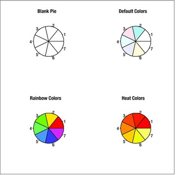
Figure 8-1. Illustration of a few of R’s color palettes

In addition to learning about the color palettes, you just learned how to display multiple graphs in the R Graphics Device. Examine Figure 8-2 to see that you can copy and save the output, as well as print it. To access these options, just right-click anywhere in the Graphics Device window.

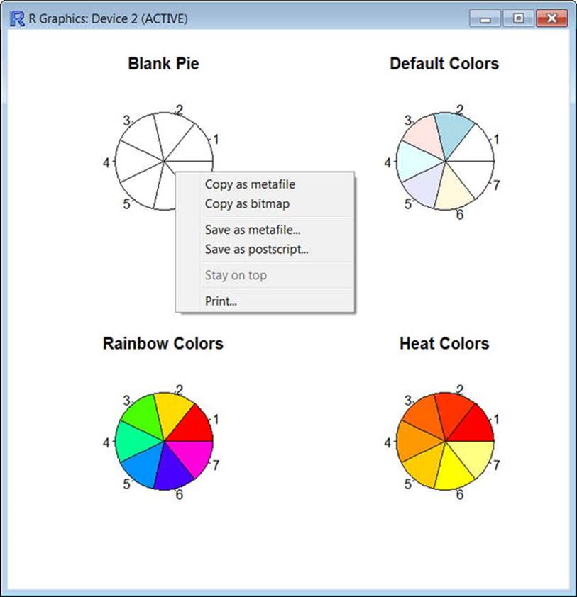
Figure 8-2. R allows you to copy, save, and print graphics

Recipe 8-2. Using the Standard Graphs

Problem

Many people are visual learners and thinkers. Numbers are wonderful, and I like playing with numbers and “crunching” them, but I really like to turn them into pictures, both mental and physical. The trite expression that a picture is worth a thousand words has a ring of truth to it.

Every statistics book in my library has a chapter on the graphical display of data. This is usually the second or third chapter in the book, because graphs are part of descriptive statistics, or what Tukey called exploratory data analysis. You have seen frequency distributions, histograms, pie charts, and bar charts (including clustered bar charts) in earlier chapters. In the remaining recipes in Chapter 8, you learn to produce line graphs, scatterplots, and various exploratory graphs and plots. We will use ggplot2 for most of the graphics in this chapter.

Solution

First, let us review some principles of good graphics before illustrating the various graphs that I just listed. Here are Tufte’s principles of graphical integrity (www.asq0511.org/Presentations/1298/sld008.htm):

· The physical area on the graphic should be directly proportional to the number represented.

· The data and important events should be labeled and explained on the graphic.

· The graphic should show variation in the data, not design variation.

· Time series displays of money should use deflated and standardized units.

· The number of chart dimensions should not exceed the number of data dimension.

· Do not quote data out of context.

Histograms

The bars in a histogram represent the frequencies of the observations. Because there is an underlying continuum, the bars should touch. Histograms are one of the most common and most meaningful ways to display simple and grouped frequency distributions.

Here is an example of a histogram taken from the ggplot2 documentation. In keeping with Tufte’s principles, I added a descriptive title. The code follows. The data for more 58,788 movies ship with ggplot2. The rating is based on International Movie Database (IMDB) user votes and can range from 1 to a perfect 10. We take a sample of 1,000 to keep our example manageable. The set.seed function allows us to generate pseudorandom numbers that we can replicate should we want to use the same example again. This is useful for various purposes; in this case, for sampling from a larger dataset. See Figure 8-3 for the histogram.

> library(ggplot2)
> set.seed(5689)
> movies <- movies[sample(nrow(movies), 1000), ]
> qplot(rating, data=movies, geom="histogram", main = "Movie Ratings")

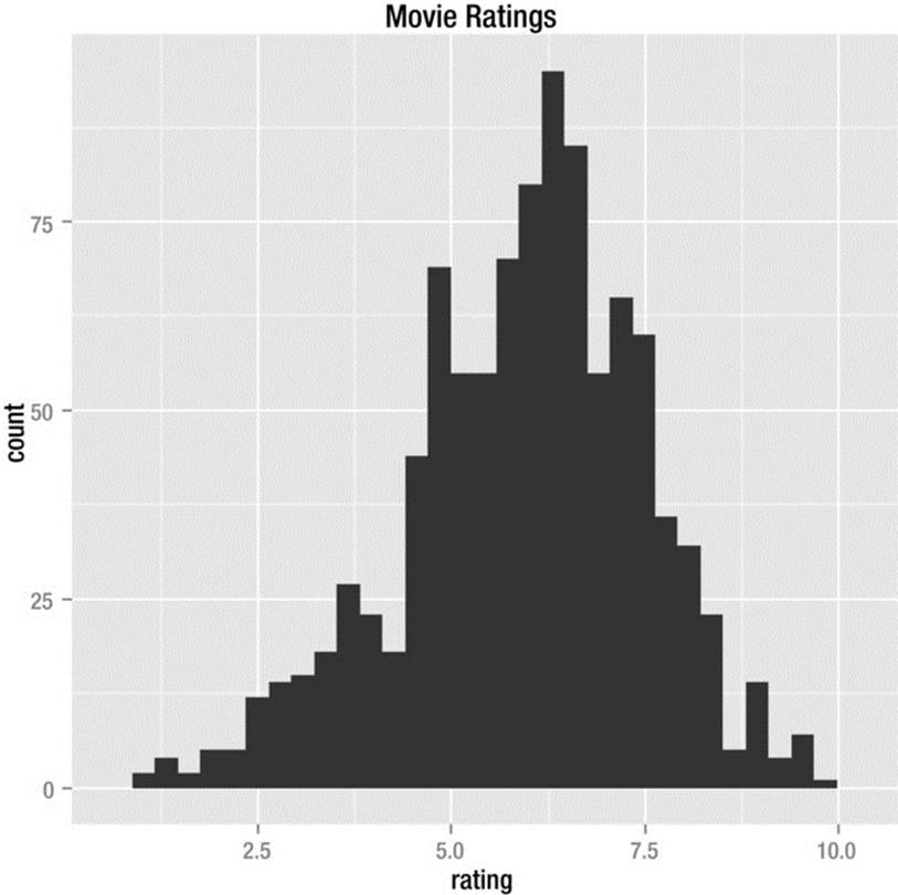
Figure 8-3. Histogram produced by ggplot2

Bar Charts

Both histograms and bar charts are produced by the geom_bar() function in ggplot2. Here are some actual expense data from one of my recent conference trips. First I create a data frame called df, which contains the meal and prices. Then I download ggplot2 using the commandinstall.packages("ggplot2"), followed by library("ggplot2") after the download is completed.

The aes() function creates the “aesthetic” for the bar chart. The default legend is redundant in this case, but can be removed by setting guides(fill = FALSE). We define the bar chart by telling R what the axes are, as well as what variable to fill. The stat = "identity"option specifies that that the bars should represent the actual values in the data frame. The default is stat = "bin", which causes the bars to represent frequencies. The completed bar chart appears in Figure 8-4.

> df
Meal Price
1 Breakfast 13.98
2 Lunch 21.52
3 Dinner 37.52
> barChart<- ggplot(df)
> barChart <- barChart +geom_bar(aes(x=Meal,y=Price, fill=Meal), stat ="identity")
> barChart + ggtitle("Meal Expenses")
> barChart + guides(fill = FALSE)

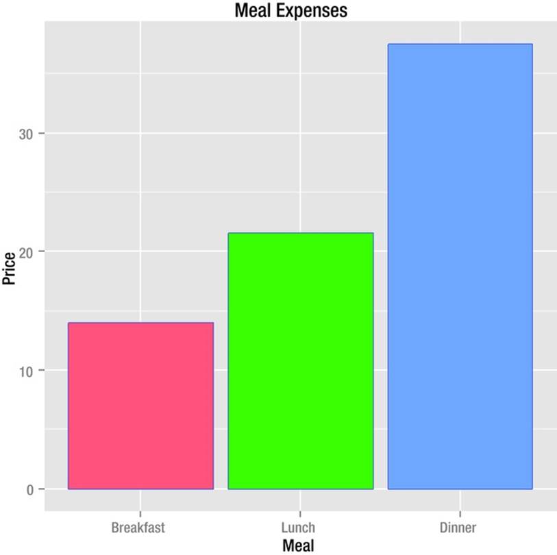
Figure 8-4. Bar chart produced by ggplot2

Line Graphs

We use line graphs to display the change in a variable or variables over time. A common example is the change in the closing price of a stock. A frequency polygon is also a kind of line graph. The following data are from the Yahoo! Finance web site. The data include the opening, high, low, closing, volume, and adjusted closing prices of Starbucks stock for the year 2013. I added an index number for the 252 days in the dataset.

> head(starbucks)
date open high low close volume adj_close number
1 1/2/2013 54.59 55.00 54.26 55.00 6633800 53.88 1
2 1/3/2013 55.07 55.61 55.00 55.37 7335200 54.24 2
3 1/4/2013 55.53 56.00 55.31 55.69 5455700 54.55 3
4 1/7/2013 55.40 55.79 55.01 55.72 4360000 54.58 4
5 1/8/2013 55.58 55.72 55.07 55.62 4806700 54.48 5
6 1/9/2013 55.89 55.90 54.33 54.63 8339200 53.51 6

We can use the qplot() function in ggplot2 for most basic graphs. See the syntax as follows. Note that the geom type is specified as a character string. The finished line graph appears in Figure 8-5.

> qplot(starbucks$number, starbucks$adj_close, geom="line", main="Starbucks Closing Price")

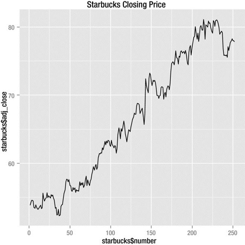
Figure 8-5. Starbucks closing stock prices for the year 2013

Scatterplots

The scatterplot is the default in ggplot2 if no geom is specified. This is consistent with the base version of R, which will produce a scatterplot when you plot two variables without further specification. Let us see how the Starbucks volumes relate to the date. Remember the xlab and ylabarguments are used to specify the labels for the x and y axes.

> qplot(starbucks$number, starbucks$volume, xlab = "date", ylab = "volume", main = "Starbucks Volume by Date")

The scatterplot appears in Figure 8-6. There is no apparent relationship between the date and the volume.

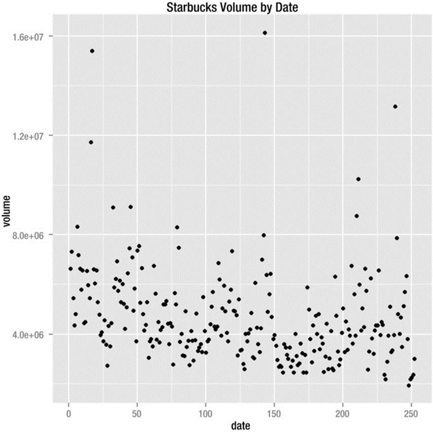
Figure 8-6. Scatterplot of Starbucks volume by date

Recipe 8-3. Using Graphics for Exploratory Data Analysis

Problem

According to John Tukey’s preface to Exploratory Data Analysis (Pearson, 1977): “Once upon a time, statisticians only explored. Then they learned to confirm exactly—to confirm a few things exactly, each under very specific circumstances. As they emphasized exact confirmation, their techniques inevitably became less flexible.”

Tukey believed that exploratory data analysis is “detective work,” and I agree. The two most common graphical tools for exploratory data analysis are the stem-and-leaf plot and the boxplot. These tools do help you see another, deeper layer in the data. The boxplot, in particular, is very useful for visualizing the shape of the data, as well as the presence of outliers. In addition to these plots, we will examine the dot plot (of which there are a couple of varieties).

Solution

A boxplot is a visual representation of the Tukey five-number summary of a dataset. These numbers are the minimum, the first quartile, the median, the third quartile, and the maximum. Tukey originally called the plot a “box and whiskers” plot.

Side-by-side boxplots are very handy for comparing two or more groups. The following example uses the PlantGrowth data frame that comes with the base version of R. The data represent the weights of 30 plants divided into three groups on the basis of a control condition and two treatment conditions:

> summary(PlantGrowth)
weight group
Min. :3.590 ctrl:10
1st Qu.:4.550 trt1:10
Median :5.155 trt2:10
Mean :5.073
3rd Qu.:5.530
Max. :6.310

Here is how to make side-by-side boxplots for the three groups using qplot(). See the graphics output in Figure 8-7, where you will note the presence of two outliers in the trt1 group.

> boxPlot <- ggplot(PlantGrowth, aes(x=group, y=weight)) + geom_boxplot()
> boxPlot

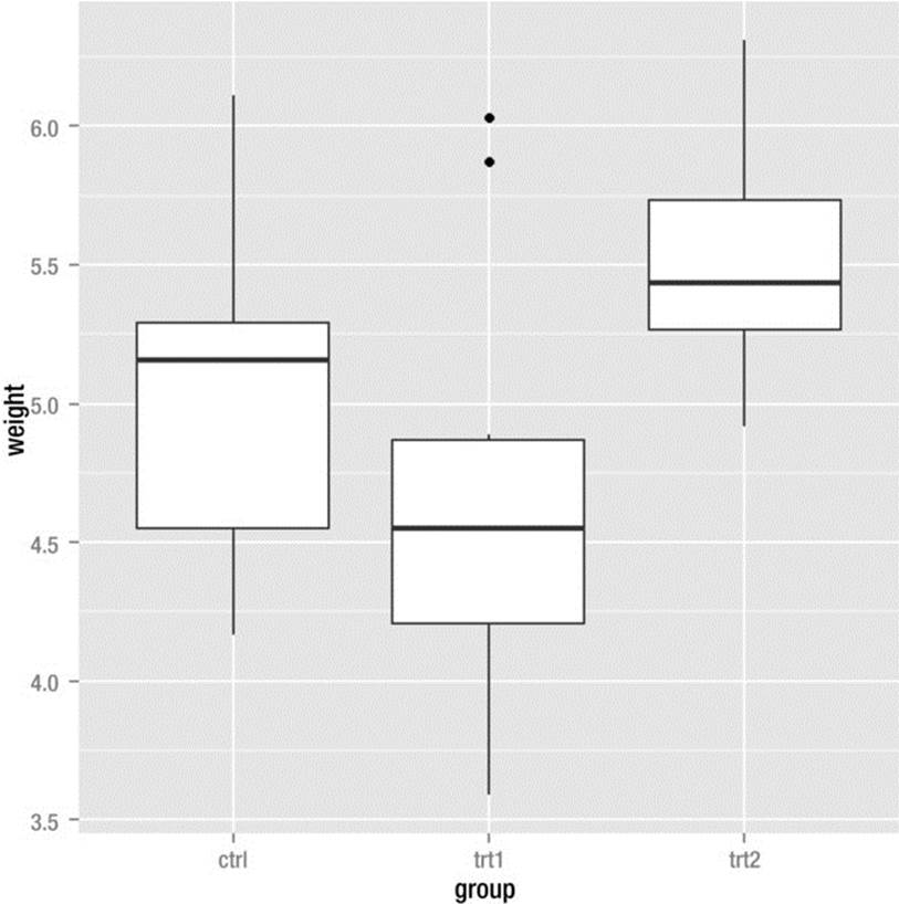
Figure 8-7. Side-by-side boxplots

I retrieved the following information from the Internet. The data include the location (the 50 US states plus Washington, DC), the region, the 2013 population, the percentage of the population with PhDs, the per capita income in 2012, the total number of PhDs awarded in that state or location during 2012, and the breakdown of these degrees by male and female. The data are part of a much larger database managed by the National Science Foundation.

> head(phds)
location region pop2013 phdPct income total maleTot femaleTot
1 Alabama southEast 4833722 0.0134 35625 648 328 320
2 Alaska nonContiguous 735132 0.0068 46778 50 29 21
3 Arizona west 6626624 0.0134 35979 888 491 397
4 Arkansas southEast 2959373 0.0066 34723 194 110 84
5 California west 38332521 0.0157 44980 6035 3423 2612
6 Colorado central 5268367 0.0154 45135 809 427 382

It would be interesting to see if there is a positive correlation between the percentage of the population with PhDs and the per capita income. There is.

> cor.test(phds$phdPct, phds$income)

Pearson's product-moment correlation

data: phds$phdPct and phds$income
t = 2.3124, df = 49, p-value = 0.025
alternative hypothesis: true correlation is not equal to 0
95 percent confidence interval:
0.0416852 0.5423665
sample estimates:
cor
0.3136656

The correlation of r = .31 is statistically significant at p = .025, but not particularly large. Squaring the correlation coefficient gives us the “coefficient of determination,” which shows the percentage of variance overlap between the per capita income and the percentage of PhDs graduated from a state. We can estimate that about 9.8% of the variation in per capita income can be predicted by knowing the percentage of PhDs who graduated in that state. However, the correlation is misleading, as you will see when we determine there are outliers throwing off the relationship. As indicated, we can use ggplot2 to produce a very nice box plot to determine the presence of the outliers. To make a boxplot for a single variable, you must add a fake x grouping variable to the aesthetic. See the following code and the resulting boxplot, which reveals four high outliers, one of them extreme (see Figure 8-8). We use scale_x_discrete(breaks = NULL to remove the unwanted zero that appears on the x axis of the plot.

> plot <- ggplot(phds, aes(x = factor(0), y = phdPct))+ geom_boxplot() + xlab("")
> plot <- plot + scale_x_discrete(breaks = NULL)
> plot

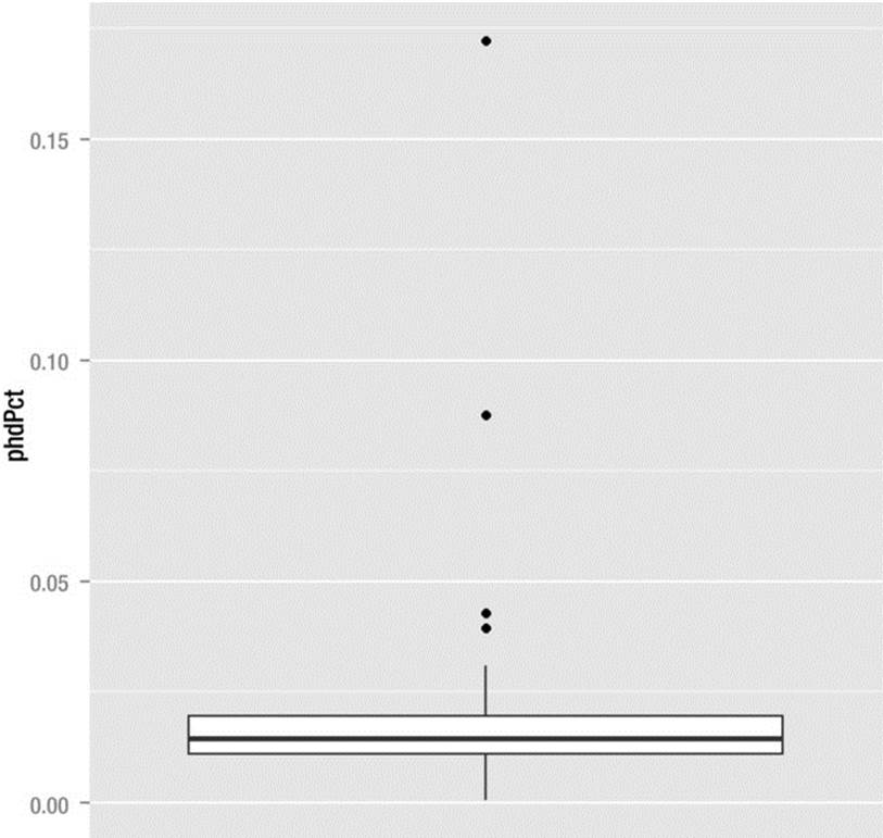
Figure 8-8. Boxplot reveals four outliers

The four locations with the highest percentages of PhDs are the District of Columbia, Massachusetts, Washington, and Wisconsin. With these locations taken out of the data, the correlation becomes slightly higher:

> cor.test(data = phds, x = phds$phdPct, y = phds$income)

Pearson's product-moment correlation

data: phds$phdPct and phds$income
t = 2.4334, df = 44, p-value = 0.01909
alternative hypothesis: true correlation is not equal to 0
95 percent confidence interval:
0.06011174 0.57700935
sample estimates:
cor
0.3443999

A scatterplot also reveals that with the outliers removed, there is basically a linear relationship between the percent of PhDs and the per capita income in a state. We can still account for only 11.9% of the variation in income, however (see Figure 8-9, in which I used ggplot to add the line of best fit). The inclusion of geom_point() adds the required layer to the scatterplot to make it visible in the R Graphics Device. The fit line is added by stat_smooth, which plots a smoother—in this case, a linear model— on the scatterplot.

> plot <- ggplot(phds,aes(phdPct, income)) + geom_point()
> plot <- plot + stat_smooth(method = "lm", se = FALSE)
> plot

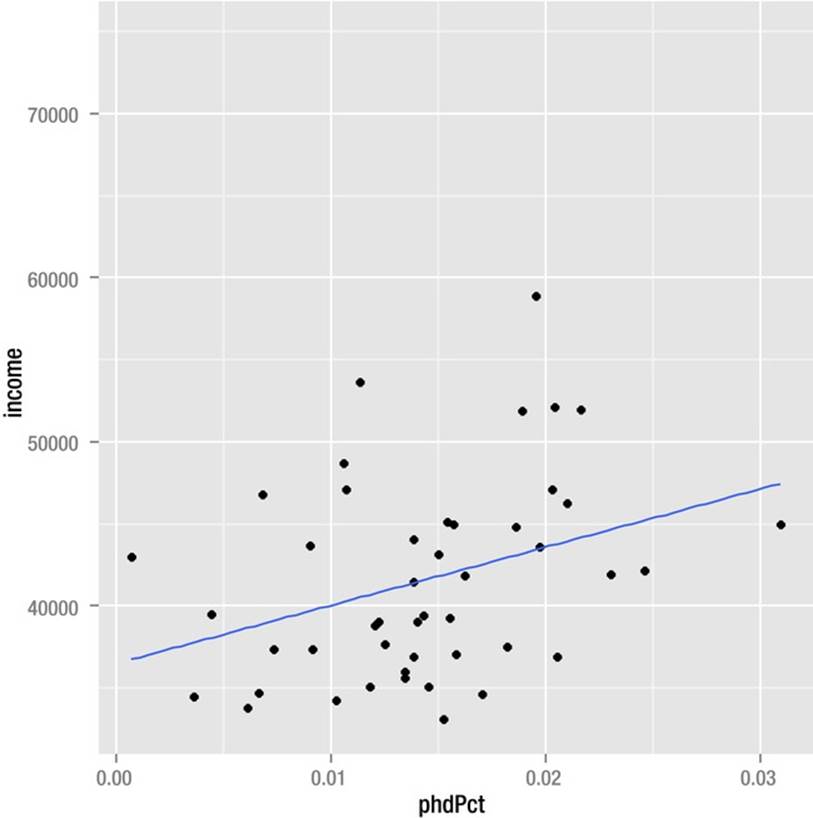
Figure 8-9. Scatterplot with line of best fit added

Stem-and-leaf plots are a semigraphical way to show the frequencies in a dataset. The stems are the leading digit(s) and the leaves are the trailing digits. A stem-and-leaf plot (also known as a stemplot) shows every value in the dataset, preserving what I call its “granularity.” The stem-and-leaf plot is not available in ggplot2, but it is in the base version of R.

One of my favorite R datasets is faithful, which lists the waiting time between eruptions and the duration of the eruptions of the Old Faithful geyser in Yellowstone National Park. Let us produce a stem-and-leaf plot of the waiting times. Because there are so many observations, R created separate bins for the trailing digits 0–4 and for 5–9 in a split stem-and-leaf plot. Clearly, if the stem-and-leaf plot were rotated 90 degrees counterclockwise, it would resemble a grouped frequency histogram. Unlike other graphs, the stem-and-leaf plot is displayed in the R Console.

> stem(faithful$waiting)

The decimal point is 1 digit(s) to the right of the |

4 | 3
4 | 55566666777788899999
5 | 00000111111222223333333444444444
5 | 555555666677788889999999
6 | 00000022223334444
6 | 555667899
7 | 00001111123333333444444
7 | 555555556666666667777777777778888888888888889999999999
8 | 000000001111111111111222222222222333333333333334444444444
8 | 55555566666677888888999
9 | 00000012334
9 | 6

Dotplots are another very good way to preserve the granularity of the dataset. The newest release of the ggplot2 package has dotplots, but, at least according to Twitter, will not have stem-and-leaf plots any time soon. As it materializes, there are different kinds of dotplots. The frequency dotplot was described by Leland Wilkinson, the mastermind behind the grammar of graphics. There is also a version of the dotplot developed by William Cleveland as an alternative to bar charts. See the completed Wilkinson dotplot in Figure 8-10. For each aesthetic used to create a plot in ggplot, one must supply the proper “geom” to produce the required layer.

> ggplot(faithful, aes(x = waiting)) + geom_dotplot()
stat_bindot: binwidth defaulted to range/30. Use 'binwidth = x' to adjust this.

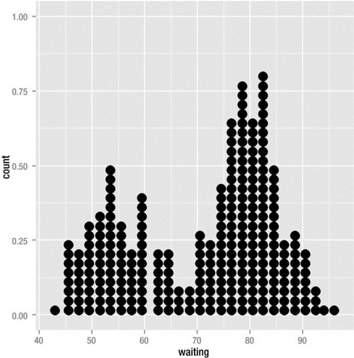
Figure 8-10. Dotplot of waiting times between eruptions of Old Faithful

Recipe 8-4. Using Graphics for Data Visualization

Problem

As was mentioned in the introduction to this chapter, data visualization is not the same thing as a graph. Certain graphs discussed in the other recipes in this chapter are useful for visualization. In Recipe 8-4, for example, boxplots and scatterplots can quickly tell us something about the relationship between variables and about the presence and the effect of outliers. Similarly, there are many other diagnostic plots that help us delve deeper into the unseen properties of the data.

Data visualization is becoming increasingly important, and also includes the visualization of ideas and concepts. For example the word cloud is an interesting way to visualize the occurrences of words or references in a text or a web site. We will cover word clouds in Chapter 14, but for now, let’s use ggplot2 and learn how to produce maps, and then populate them with data to help us visualize the information more effectively.

Solution

R is an effective visualization tool with the ggplot2 package installed. One of the best uses of ggplot2 is to create maps that help to visualize one or more attributes of a geographical location. According to Hadley Wickham, the grammar of graphics requires that every plot must consist of five components:

· a default dataset with aesthetic mappings

· one or more layers, each with a geometric object, a statistical transformation, and a dataset with aesthetic mappings

· a scale for each aesthetic mapping

· a coordinate system

· a facet specification

The purpose of the ggmap package is to take a downloaded map image and plot it as a context layer in ggplot2. The user can then add layers of data, statistics, or models to the map. With ggmap, the x aesthetic is fixed to longitude, the y aesthetic is fixed to latitude, and the coordinate system is fixed to the Mercator projection.

Compare a table of the level of unemployment by US county in 2009 to a map with the same information (see Figure 8-11). It is obvious that the map allows visualization that is not possible from the raw data.

> head(unemp)
fips pop unemp colorBuckets
1 1001 23288 9.7 5
2 1003 81706 9.1 5
3 1005 9703 13.4 6
4 1007 8475 12.1 6
5 1009 25306 9.9 5
6 1011 3527 16.4 6
> tail(unemp)
fips pop unemp colorBuckets
3213 72143 12060 16.3 6
3214 72145 20122 17.6 6
3215 72147 3053 27.7 6
3216 72149 9141 19.8 6
3217 72151 11066 24.1 6
3218 72153 16275 16.0 6

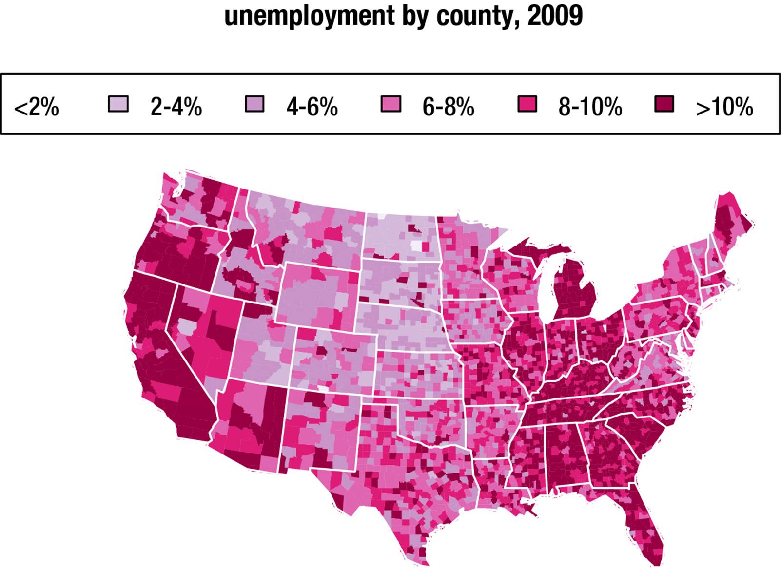
Figure 8-11. Unemployment by county, 2009

The following example is based on the Harvard University Center for Computational Biology’s course on spatial maps and geocoding in R (http://bcb.dfci.harvard.edu/~aedin/courses/R/CDC/maps.html). Here is how the map was constructed. Note the use of color to add visual appeal to the map. We cut the unemployment statistics into five categories, plot the map, and then “fill the bucket” for each US county. The result is a visually attractive and informative overview of unemployment at the state and county levels. FIPS are Federal Information Processing Standards five-digit codes assigned by the National Institute of Standards and Technology (NIST) to specify US states (the first two digits) and counties (the last three digits).

data(unemp)
data(county.fips)

# Plot unemployment by country
colors = c("#F1EEF6", "#D4B9DA", "#C994C7", "#DF65B0", "#DD1C77",
"#980043")
head(unemp)
unemp$colorBuckets <- as.numeric(cut(unemp$unemp, c(0, 2, 4, 6, 8,
10, 100)))
colorsmatched <- unemp$colorBuckets[match(county.fips$fips, unemp$fips)]

map("county", col = colors[colorsmatched], fill = TRUE, resolution = 0,
lty = 0, projection = "polyconic")
## Loading required package: mapproj

# Add border around each State
map("state", col = "white", fill = FALSE, add = TRUE, lty = 1, lwd = 0.2,
projection = "polyconic")
title("unemployment by county, 2009")

leg.txt <- c("<2%", "2-4%", "4-6%", "6-8%", "8-10%", ">10%")
legend("topright", leg.txt, horiz = TRUE, fill = colors)

Of course, we can visualize other things besides unemployment statistic by US county. For example, here is a map of the southeastern United States (see Figure 8-12). I used ggplot to build the map, and the geocode() function to look up the latitude and longitude values for a state university in each state. I then looked up the fall 2013 enrollment for each school and plotted the schools’ locations along with a label and the total enrollment, which shows as a larger filled circle for larger enrollments. Here is the code that accomplished this. Only a couple of the geocodes are shown to illustrate.

> geocode("university of georgia")
Information from URL : http://maps.googleapis.com/maps/api/geocode/json?address=university+of+georgia&sensor=false
Google Maps API Terms of Service : http://developers.google.com/maps/terms
lon lat
1 -83.37732 33.94801
> geocode("university of alabama")

Information from URL : http://maps.googleapis.com/maps/api/geocode/json?address=university+of+alabama&sensor=false

Google Maps API Terms of Service : http://developers.google.com/maps/terms
lon lat
1 -87.54743 33.21444

> mydata
school long lat enrollment label
1 University of Alabama -87.54743 33.21444 34852 UA
2 University of Florida -82.34639 29.64526 49042 UF
3 University of Georgia -83.37732 33.94801 34536 UGA
4 University of Kentucky -84.50397 38.03065 28037 UK
5 University of Mississippi -89.53844 34.36473 22286 Ole Miss
6 University of North Carolina at Chapel Hill -79.04691 35.90491 28136 UNC
7 University of South Carolina -81.02743 33.99611 32848 USC
8 University of Tennessee at Knoxville -83.92074 35.96064 27171 UTK
9 University of Virginia -78.50798 38.03355 23464 UVA

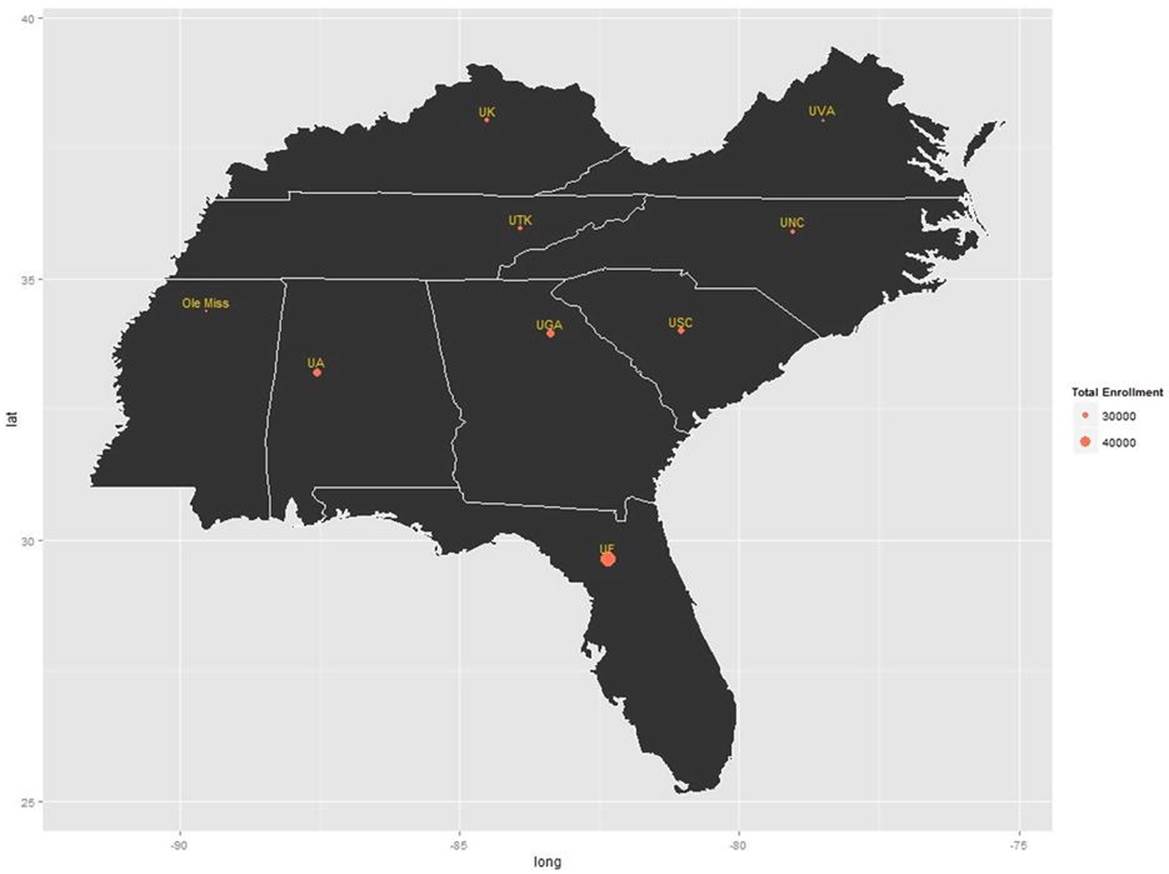
Figure 8-12. Universities in the southeast and their enrollments

Now, here is the code for making the map:

library(ggplot2)
library(maps)
#load us map data
all_states <- map_data("state")
southeast <- subset(all_states, region %in% c("florida", "georgia", "south carolina", "north carolina", "virginia","kentucky","tennessee","mississippi","alabama"))
p <- ggplot()
p <- p + geom_polygon(data=southeast, aes(x=long, y=lat, group = group), color="white" )
p <- p + geom_point( data=mydata, aes(x=long, y=lat, size = enrollment), color="coral1") + scale_size(name="Total Enrollment")
p <- p + geom_text( data=mydata, hjust=0.5, vjust=-0.5, aes(x=long, y=lat, label=label), color="gold2", size=4 )

And finally, the map itself (see Figure 8-12).