Time Series Databases: New Ways to Store and Access Data (2014)
Chapter 3. Storing and Processing Time Series Data
As we mentioned in previous chapters, a time series is a sequence of values, each with a time value indicating when the value was recorded. Time series data entries are rarely amended, and time series data is often retrieved by reading a contiguous sequence of samples, possibly after summarizing or aggregating the retrieved samples as they are retrieved. A time series database is a way to store multiple time series such that queries to retrieve data from one or a few time series for a particular time range are particularly efficient. As such, applications for which time range queries predominate are often good candidates for implementation using a time series database. As previously explained, the main topic of this book is the storage and processing of large-scale time series data, and for this purpose, the preferred technologies are NoSQL non-relational databases such as Apache HBase or MapR-DB.
Pragmatic advice for practical implementations of large-scale time series databases is the goal of this book, so we need to focus in on some basic steps that simplify and strengthen the process for real-world applications. We will look briefly at approaches that may be useful for small or medium-sized datasets and then delve more deeply into our main concern: how to implement large-scale TSDBs.
To get to a solid implementation, there are a number of design decisions to make. The drivers for these decisions are the parameters that define the data. How many distinct time series are there? What kind of data is being acquired? At what rate is the data being acquired? For how long must the data be kept? The answers to these questions help determine the best implementation strategy.
ROADMAP TO KEY IDEAS IN THIS CHAPTER
Although we’ve already mentioned some central aspects to handling time series data, the current chapter goes into the most important ideas underlying methods to store and access time series in more detail and more deeply than previously. Chapter 4 then provides tips for how best to implement these concepts using existing open source software. There’s a lot to absorb in these two chapters. So that you can better keep in mind how the key ideas fit together without getting lost in the details, here’s a brief roadmap of this chapter:
§ Flat files
§ Limited utility for time series; data will outgrow them, and access is inefficient
§ True database: relational (RDBMS)
§ Will not scale well; familiar star schema inappropriate
§ True database: NoSQL non-relational database
§ Preferred because it scales well; efficient and rapid queries based on time range
§ Basic design
§ Unique row keys with time series IDs; column is a time offset
§ Stores more than one time series
§ Design choices
§ Wide table stores data point-by-point
§ Hybrid design mixes wide table and blob styles
§ Direct blob insertion from memory cache
Now that we’ve walked through the main ideas, let’s revisit them in some detail to explain their significance.
Simplest Data Store: Flat Files
You can extend this very simple design a bit to something slightly more advanced by using a more clever file format, such as the columnar file format Parquet, for organization. Parquet is an effective and simple, modern format that can store the time and a number of optional values.Figure 3-1 shows two possible Parquet schemas for recording time series. The schema on the left is suitable for special-purpose storage of time series data where you know what measurements are plausible. In the example on the left, only the four time series that are explicitly shown can be stored (tempIn, pressureIn, tempOut, pressureOut). Adding another time series would require changing the schema. The more abstract Parquet schema on the right in Figure 3-1 is much better for cases where you may want to embed more metadata about the time series into the data file itself. Also, there is no a priori limit on the number or names of different time series that can be stored in this format. The format on the right would be much more appropriate if you were building a time series library for use by other people.
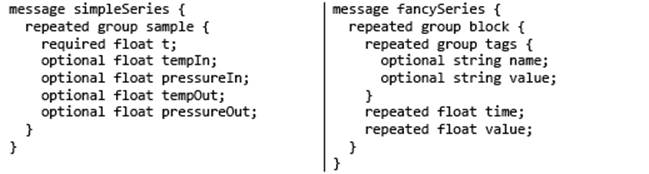
Figure 3-1. Two possible schemas for storing time series data in Parquet. The schema on the left embeds knowledge about the problem domain in the names of values. Only the four time series shown can be stored without changing the schema. In contrast, the schema on the right is more flexible; you could add additional time series. It is also a bit more abstract, grouping many samples for a single time series into a single block.
Such a simple implementation of a time series—especially if you use a file format like Parquet—can be remarkably serviceable as long as the number of time series being analyzed is relatively small and as long as the time ranges of interest are large with respect to the partitioning time for the flat files holding the data.
While it is fairly common for systems to start out with a flat file implementation, it is also common for the system to outgrow such a simple implementation before long. The basic problem is that as the number of time series in a single file increases, the fraction of usable data for any particular query decreases, because most of the data being read belongs to other time series.
Likewise, when the partition time is long with respect to the average query, the fraction of usable data decreases again since most of the data in a file is outside the time range of interest. Efforts to remedy these problems typically lead to other problems. Using lots of files to keep the number of series per file small multiplies the number of files. Likewise, shortening the partition time will multiply the number of files as well. When storing data on a system such as Apache Hadoop using HDFS, having a large number of files can cause serious stability problems. Advanced Hadoop-based systems like MapR can easily handle the number of files involved, but retrieving and managing large numbers of very small files can be inefficient due to the increased seek time required.
To avoid these problems, a natural step is to move to some form of a real database to store the data. The best way to do this is not entirely obvious, however, as you have several choices about the type of database and its design. We will examine the issues to help you decide.
Moving Up to a Real Database: But Will RDBMS Suffice?
Even well-partitioned flat files will fail you in handling your large-scale time series data, so you will want to consider some type of true database. When first storing time series data in a database, it is tempting to use a so-called star schema design and to store the data in a relational database (RDBMS). In such a database design, the core data is stored in a fact table that looks something like what is shown in Figure 3-2.
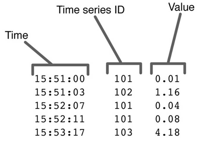
Figure 3-2. A fact table design for a time series to be stored in a relational database. The time, a series ID, and a value are stored. Details of the series are stored in a dimension table.
In a star schema, one table stores most of the data with references to other tables known as dimensions. A core design assumption is that the dimension tables are relatively small and unchanging. In the time series fact table shown in Figure 3-2, the only dimension being referenced is the one that gives the details about the time series themselves, including what measured the value being stored. For instance, if our time series is coming from a factory with pumps and other equipment, we might expect that several values would be measured on each pump such as inlet and outlet pressures and temperatures, pump vibration in different frequency bands, and pump temperature. Each of these measurements for each pump would constitute a separate time series, and each time series would have information such as the pump serial number, location, brand, model number, and so on stored in a dimension table.
A star schema design like this is actually used to store time series in some applications. We can also use a design like this in most NoSQL databases as well. A star schema addresses the problem of having lots of different time series and can work reasonably well up to levels of hundreds of millions or billions of data points. As we saw in Chapter 1, however, even 19th century shipping data produced roughly a billion data points. As of 2014, the NASDAQ stock exchange handles a billion trades in just over three months. Recording the operating conditions on a moderate-sized cluster of computers can produce half a billion data points in a day.
Moreover, simply storing the data is one thing; retrieving it and processing it is quite another. Modern applications such as machine learning systems or even status displays may need to retrieve and process as many as a million data points in a second or more.
While relational systems can scale into the lower end of these size and speed ranges, the costs and complexity involved grows very fast. As data scales continue to grow, a larger and larger percentage of time series applications just don’t fit very well into relational databases. Using the star schema but changing to a NoSQL database doesn’t particularly help, either, because the core of the problem is in the use of a star schema in the first place, not just the amount of data.
NoSQL Database with Wide Tables
The core problem with the star schema approach is that it uses one row per measurement. One technique for increasing the rate at which data can be retrieved from a time series database is to store many values in each row. With some NoSQL databases such as Apache HBase or MapR-DB, the number of columns in a database is nearly unbounded as long as the number of columns with active data in any particular row is kept to a few hundred thousand. This capability can be exploited to store multiple values per row. Doing this allows data points to be retrieved at a higher speed because the maximum rate at which data can be scanned is partially dependent on the number of rows scanned, partially on the total number of values retrieved, and partially on the total volume of data retrieved. By decreasing the number of rows, that part of the retrieval overhead is substantially cut down, and retrieval rate is increased. Figure 3-3 shows one way of using wide tables to decrease the number of rows used to store time series data. This technique is similar to the default table structure used in OpenTSDB, an open source database that will be described in more detail in Chapter 4. Note that such a table design is very different from one that you might expect to use in a system that requires a detailed schema be defined ahead of time. For one thing, the number of possible columns is absurdly large if you need to actually write down the schema.
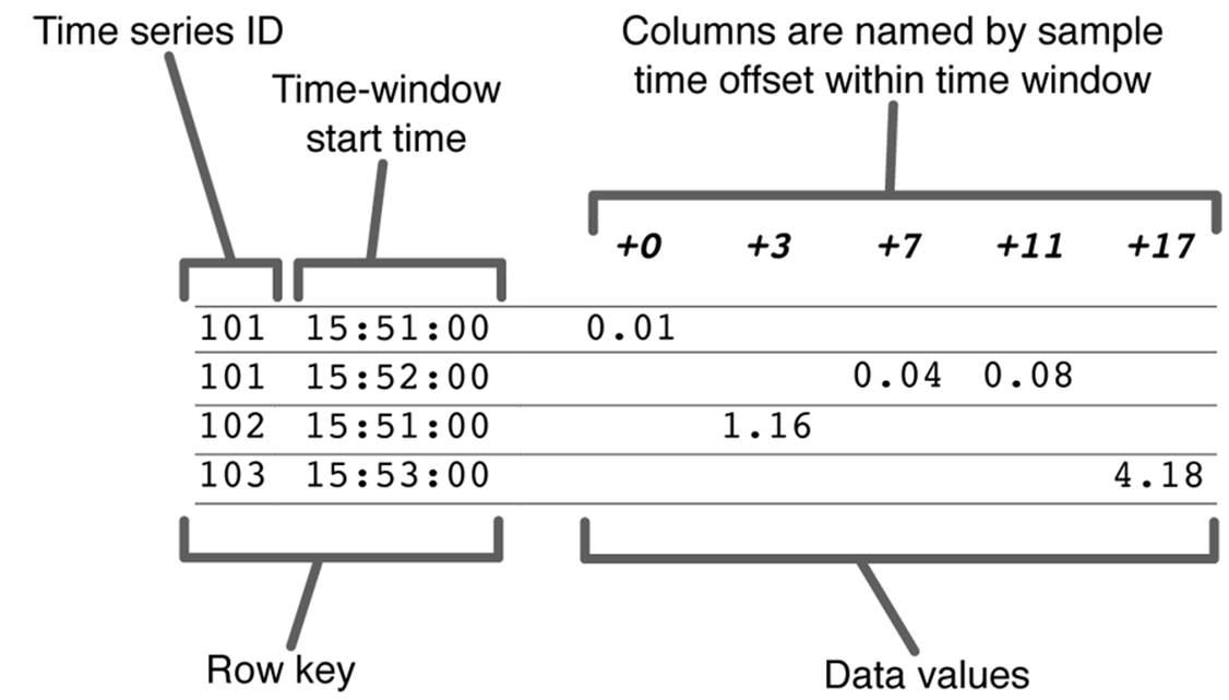
Figure 3-3. Use of a wide table for NoSQL time series data. The key structure is illustrative; in real applications, a binary format might be used, but the ordering properties would be the same.
Because both HBase and MapR-DB store data ordered by the primary key, the key design shown in Figure 3-3 will cause rows containing data from a single time series to wind up near one another on disk. This design means that retrieving data from a particular time series for a time range will involve largely sequential disk operations and therefore will be much faster than would be the case if the rows were widely scattered. In order to gain the performance benefits of this table structure, the number of samples in each time window should be substantial enough to cause a significant decrease in the number of rows that need to be retrieved. Typically, the time window is adjusted so that 100–1,000 samples are in each row.
NoSQL Database with Hybrid Design
The table design shown in Figure 3-3 can be improved by collapsing all of the data for a row into a single data structure known as a blob. This blob can be highly compressed so that less data needs to be read from disk. Also, if HBase is used to store the time series, having a single column per row decreases the per-column overhead incurred by the on-disk format that HBase uses, which further increases performance. The hybrid-style table structure is shown in Figure 3-4, where some rows have been collapsed using blob structures and some have not.
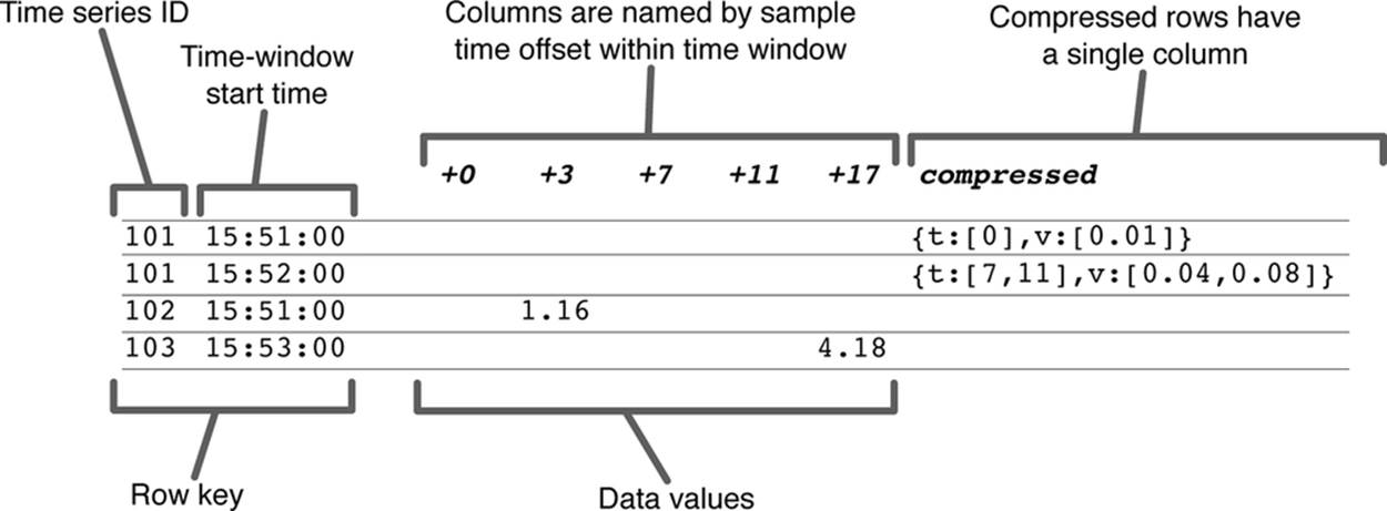
Figure 3-4. In the hybrid design, rows can be stored as a single data structure (blob). Note that the actual compressed data would likely be in a binary, compressed format. The compressed data are shown here in JSON format for ease of understanding.
Data in the wide table format shown in Figure 3-3 can be progressively converted to the compressed format (blob style) shown in Figure 3-4 as soon as it is known that little or no new data is likely to arrive for that time series and time window. Commonly, once the time window ends, new data will only arrive for a few more seconds, and the compression of the data can begin. Since compressed and uncompressed data can coexist in the same row, if a few samples arrive after the row is compressed, the row can simply be compressed again to merge the blob and the late-arriving samples.
The conceptual data flow for this hybrid-style time series database system is shown in Figure 3-5.
Converting older data to blob format in the background allows a substantial increase in the rate at which the renderer depicted in Figure 3-5 can retrieve data for presentation. On a 4-node MapR cluster, for instance, 30 million data points can be retrieved, aggregated and plotted in about 20 seconds when data is in the compressed form.
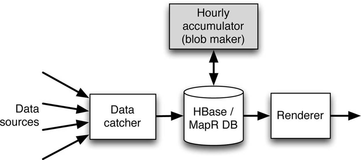
Figure 3-5. Data flow for the hybrid style of time series database. Data arrives at the catcher from the sources and is inserted into the NoSQL database. In the background, the blob maker rewrites the data later in compressed blob form. Data is retrieved and reformatted by the renderer.
Going One Step Further: The Direct Blob Insertion Design
Compression of old data still leaves one performance bottleneck in place. Since data is inserted in the uncompressed format, the arrival of each data point requires a row update operation to insert the value into the database. This row update can limit the insertion rate for data to as little as 20,000 data points per second per node in the cluster.
On the other hand, the direct blob insertion data flow diagrammed in Figure 3-6 allows the insertion rate to be increased by as much as roughly 1,000-fold. How does the direct blob approach get this bump in performance? The essential difference is that the blob maker has been moved into the data flow between the catcher and the NoSQL time series database. This way, the blob maker can use incoming data from a memory cache rather than extracting its input from wide table rows already stored in the storage tier.
The basic idea is that data is kept in memory as samples arrive. These samples are also written to log files. These log files are the “restart logs” shown in Figure 3-6 and are flat files that are stored on the Hadoop system but not as part of the storage tier itself. The restart logs allow the in-memory cache to be repopulated if the data ingestion pipeline has to be restarted.
In normal operations, at the end of a time window, new in-memory structures are created, and the now static old in-memory structures are used to create compressed data blobs to write to the database. Once the data blobs have been written, the log files are discarded. Compare the point in the data flow at which writes occur in the two scenarios. In the hybrid approach shown in Figure 3-5, the entire incoming data stream is written point-by-point to the storage tier, then read again by the blob maker. Reads are approximately equal to writes. Once data is compressed to blobs, it is again written to the database. In contrast, in the main data flow of the direct blob insertion approach shown in Figure 3-6, the full data stream is only written to the memory cache, which is fast, rather than to the database. Data is not written to the storage tier until it’s compressed into blobs, so writing can be much faster. The number of database operations is decreased by the average number of data points in each of the compressed data blobs. This decrease can easily be a factor in the thousands.
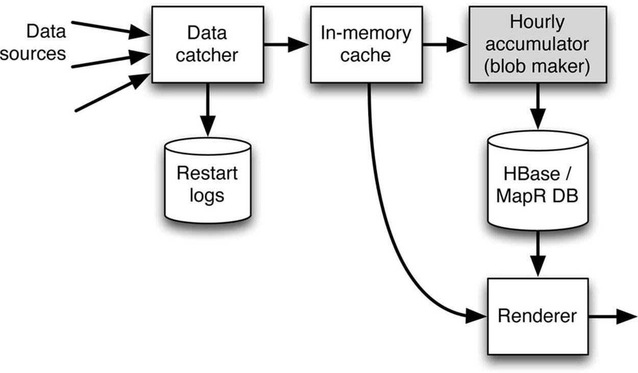
Figure 3-6. Data flow for the direct blob insertion approach. The catcher stores data in the cache and writes it to the restart logs. The blob maker periodically reads from the cache and directly inserts compressed blobs into the database. The performance advantage of this design comes at the cost of requiring access by the renderer to data buffered in the cache as well as to data already stored in the time series database.
What are the advantages of this direct blobbing approach? A real-world example shows what it can do. This architecture has been used to insert in excess of 100 million data points per second into a MapR-DB table using just 4 active nodes in a 10-node MapR cluster. These nodes are fairly high-performance nodes, with 16 cores, lots of RAM, and 12 well-configured disk drives per node, but you should be able to achieve performance within a factor of 2–5 of this level using most hardware.
This level of performance sounds like a lot of data, possibly more than most of us would need to handle, but in Chapter 5 we will show why ingest rates on that level can be very useful even for relatively modest applications.
Why Relational Databases Aren’t Quite Right
At this point, it is fair to ask why a relational database couldn’t handle nearly the same ingest and analysis load as is possible by using a hybrid schema with MapR-DB or HBase. This question is of particular interest when only blob data is inserted and no wide table data is used, because modern relational databases often have blob or array types.
The answer to this question is that a relational database running this way will provide reasonable, but not stellar, ingestion and retrieval rates. The real problem with using a relational database for a system like this is not performance, per se. Instead, the problem is that by moving to a blob style of data storage, you are giving up almost all of the virtues of a relational system. Additionally, SQL doesn’t provide a good abstraction method to hide the details of accessing of a blob-based storage format. SQL also won’t be able to process the data in any reasonable way, and special features like multirow transactions won’t be used at all. Transactions, in particular, are a problem here because even though they wouldn’t be used, this feature remains, at a cost. The requirement that a relational database support multirow transactions makes these databases much more difficult to scale to multinode configurations. Even getting really high performance out of a single node can require using a high-cost system like Oracle. With a NoSQL system like Apache HBase or MapR-DB instead, you can simply add additional hardware to get more performance.
This pattern of paying a penalty for unused features that get in the way of scaling a system happens in a number of high-performance systems. It is common that the measures that must be taken to scale a system inherently negate the virtues of a conventional relational database, and if you attempt to apply them to a relational database, you still do not get the scaling you desire. In such cases, moving to an alternative database like HBase or MapR-DB can have substantial benefits because you gain both performance and scalability.
Hybrid Design: Where Can I Get One?
These hybrid wide/blob table designs can be very alluring. Their promise of enormous performance levels is exciting, and the possibility that they can run on fault-tolerant, Hadoop-based systems such as the MapR distribution make them attractive from an operational point of view as well. These new approaches are not speculation; they have been built and they do provide stunning results. The description we’ve presented here so far, however, is largely conceptual. What about real implementations? The next chapter addresses exactly how you can realize these new designs by describing how you can use OpenTSDB, an open source time series database tool, along with special open source MapR extensions. The result is a practical implementation able to take advantage of the concepts described in this chapter to achieve high performance with a large-scale time series database as is needed for modern use cases.
All materials on the site are licensed Creative Commons Attribution-Sharealike 3.0 Unported CC BY-SA 3.0 & GNU Free Documentation License (GFDL)
If you are the copyright holder of any material contained on our site and intend to remove it, please contact our site administrator for approval.
© 2016-2026 All site design rights belong to S.Y.A.