Splunk Essentials (2015)

Chapter 6. Using the Twitter App

In the last chapter, we learned about the many apps available on Splunk. We also learned about how to obtain a Twitter API key, and how to install the app for Twitter data that is available for Splunk. In this chapter, we will use that app to create reports and dashboards based on streaming Twitter data. We will cover the following topics:

· Creating a Twitter index

· Searching Twitter data

· The built-in General Activity dashboard

· The built-in per-user Activity dashboard

· Creating dashboard panels with Twitter data

Creating a Twitter index

We'll start off this chapter by bringing in some Twitter data using the app we set up in Chapter 5, Splunk Applications. Open up Splunk and follow the steps given here:

1. Sign in and go to the Splunk home page.

2. If you've set up the app for Twitter data according to the instructions in the last chapter, your screen should look like the following image (if not, go back to the end of Chapter 5, Splunk Applications):

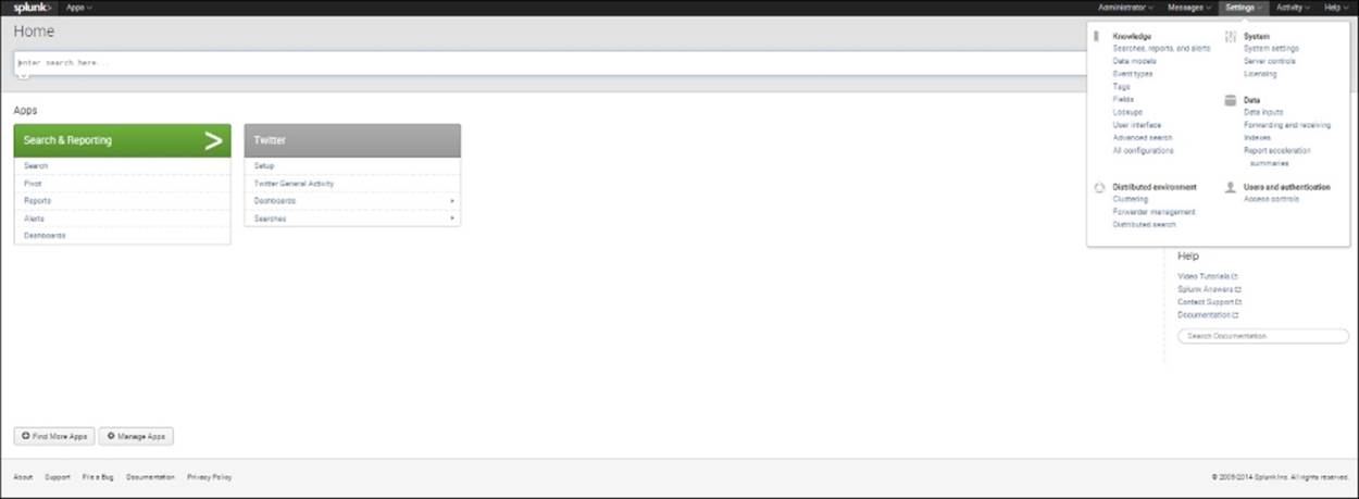
The Home Screen with the Twitter App Installed

3. Click on Setup, which is listed first under Twitter on the app.

4. You should see the API information you filled in as described in the previous chapter.

5. Check the box Enable Twitter Input, as shown in the following screenshot:

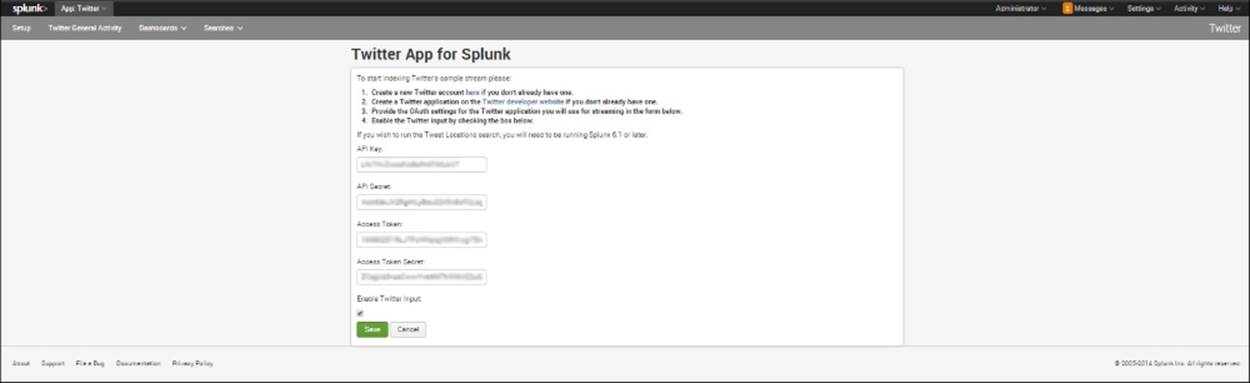
Check the Enable Twitter Input box to start the live Twitter stream

6. This will start the live Twitter stream. Remember that you will need to keep an eye on the amount of data you let in each day, as the Splunk trial license will only allow the indexing of 500 MB of data per day. Going beyond this could mean that you will lose the ability to search your data until the license has been reset or an Enterprise license is purchased. One way to keep track of the data that you are indexing is to go to the list of indexes:

1. Go to Settings.

2. Under Data, select Indexes.

3. You will see a screen like the one shown here:

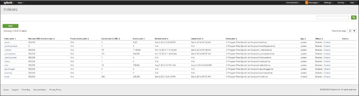
The Indexes screen

4. Notice that in the Twitter index (shown in the preceding screenshot), the event count is 423,465. In this case, each event is a tweet. Also notice that you can disable an index easily by clicking on Disable under Status. Additionally, you can see the path where the Twitter index is stored.

5. Remember that you can only index an additional 500 MB per day in the free version of Splunk Enterprise, but that you can index up to 500,000 MB in the Total Index. The event count is not limited here, just the amount of megabytes of data indexed each day.

6. One way to see how much you have used of the 500 MB allowed per day is to go to Activity, then System Activity, and under Serve, select License Usage. You will see a dashboard like the one shown in the following screenshot, which can tell you how much of the day's licensed indexing you have used up. This dashboard shows that I have used 241 MB of the .5 GB (500 MB) allowed per day:

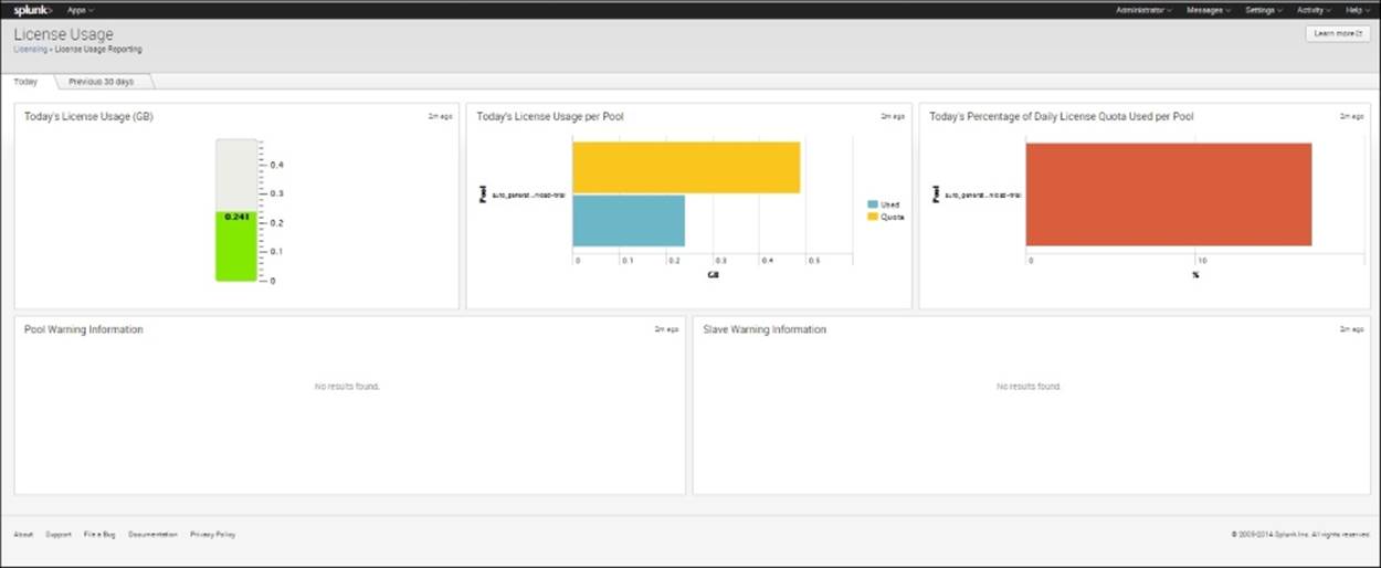
License Usage screen

Searching Twitter data

We will start here by doing a simple search of our Twitter index, which is automatically created by the app once you have enabled Twitter input (as explained previously). In our earlier searches, we used the default index (which the tutorial data was downloaded to), so we didn't have to specify the index we wanted to use. Here, we will use just the Twitter index, so we need to specify that in the search.

A simple search

Imagine that we wanted to search for tweets containing the word coffee. We could use the code presented here and place it in the search bar:

index=twitter text=*coffee*

The preceding code searches only your Twitter index and finds all the places where the word coffee is mentioned. You have to put asterisks there, otherwise you will only get the tweets with just "coffee". (Note that the text field is not case sensitive, so tweets with either "coffee" or "Coffee" will be included in the search results. There are hacks to get around this using regular expressions, but these are beyond the scope of this book.)

The asterisks are included before and after the text "coffee" because otherwise we would only get events where just "coffee" was tweeted – a rather rare occurrence, we expect. In fact, when we search our indexed Twitter data without the asterisks around coffee, we got no results.

Examining the Twitter event

Before going further, it is useful to stop and closely examine the events that are collected as part of the search. The sample tweet shown in the following screenshot shows the large number of fields that are part of each tweet. The > was clicked to expand the event:

A Twitter event

There are several items to look closely at here:

1. _time: Splunk assigns a timestamp for every event. This is done in UTC (Coordinated Universal Time) time format.

2. contributors: The value for this field is null, as are the values of many Twitter fields.

3. Retweeted_status: Notice the {+} here; in the following event list, you will see there are a number of fields associated with this, which can be seen when the + is selected and the list is expanded. This is the case wherever you see a {+} in a list of fields:

Various retweet fields

In addition to those shown previously, there are many other fields associated with a tweet. The 140 character (maximum) text field that most people consider to be the tweet is actually a small part of the actual data collected.

The implied AND

If you want to search on more than one term, there is no need to add AND as it is already implied. If, for example, you want to search for all tweets that include both the text "coffee" and the text "morning", then use:

index=twitter text=*coffee* text=*morning*

If you don't specify text= for the second term and just put *morning*, Splunk assumes that you want to search for *morning* in any field. Therefore, you could get that word in another field in an event. This isn't very likely in this case, although coffee could conceivably be part of a user's name, such as "coffeelover". But if you were searching for other text strings, such as a computer term like log or error, such terms could be found in a number of fields. So specifying the field you are interested in would be very important.

The need to specify OR

Unlike AND, you must always specify the word OR. For example, to obtain all events that mention either coffee or morning, enter:

index=twitter text=*coffee* OR text=*morning*

Finding other words used

Sometimes you might want to find out what other words are used in tweets about coffee. You can do that with the following search:

index=twitter text=*coffee* | makemv text | mvexpand text | top 30 text

This search first searches for the word "coffee" in a text field, then creates a multivalued field from the tweet, and then expands it so that each word is treated as a separate piece of text. Then it takes the top 30 words that it finds.

You might be asking yourself how you would use this kind of information. This type of analysis would be of interest to a marketer, who might want to use words that appear to be associated with coffee in composing the script for an advertisement. The following screenshot shows the results that appear (1 of 2 pages). From this search, we can see that the words love, good, and cold might be words worth considering:

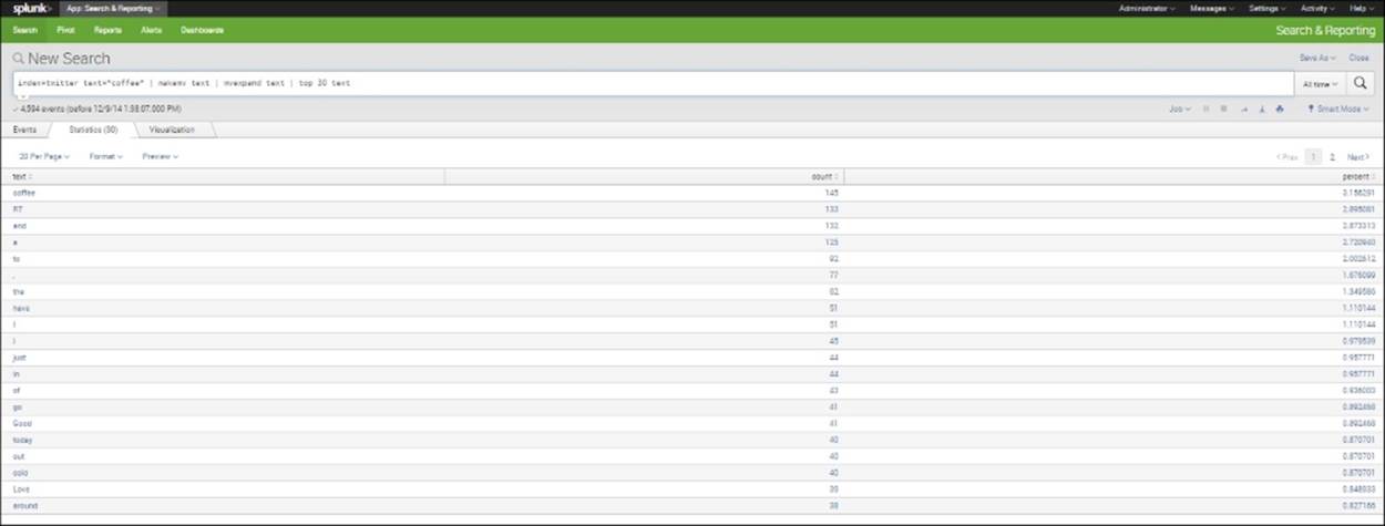
Search of top 30 text fields found with *coffee*

When you do a search like this, you will notice that there are a lot of filler words (a, to, for, and so on) that appear. You can do two things to remedy this. You can increase the limit for top words so that you can see more of the words that come up, or you can rerun the search using the following code. "Coffee" (with a capital C) is listed (on the unshown second page) separately here from "coffee". The reason for this is that while the search is not case sensitive (thus both "coffee" and "Coffee" are picked up when you search on "coffee"), the process of putting the text fields through the makemv and the mvexpand processes ends up distinguishing on the basis of case. We could rerun the search, excluding some of the filler words, using the code shown here:

index=twitter text=*coffee* | makemv text | mvexpand text | search NOT text="RT" AND NOT text="a" AND NOT text="to" AND NOT text="the" | top 30 text

Using a lookup table

Sometimes it is useful to use a lookup file to avoid having to use repetitive code. We'll present an example here that will help us with the situation presented in the preceding section. It would help us to have a list of all the small words that might be found often in a tweet just by the nature of each word's frequent use in language, so that we might eliminate them from our quest to find words that would be relevant for use in the creation of advertising. If we had a file of such small words, we could use a command indicating not to use any of these more common, irrelevant words when listing the top 30 words associated with our search topic of interest. Thus, for our search for words associated with the text "coffee", we would be interested in words like " dark", "flavorful", and "strong", but not words like "a", "the", and "then".

We can do this using a lookup command. There are three types of lookup commands, which are presented in the following table:

The command we will use here is inputlookup, because we want to reference a .csv file we can create that will include words that we want to filter out as we seek to find possible advertising words associated with coffee. Let's call the .csv file filtered_words.csv, and give it just a single text field, containing words like "is", "the", and "then". Let's rewrite the search to look like the following code:

index=twitter text=*coffee*

| makemv text | mvexpand text

| search NOT [inputlookup filtered_words | fields text ]

| top 30 text

Using the preceding code, Splunk will search our Twitter index for *coffee*, and then expand the text field so that individual words are separated out. Then it will look for words that do NOT match any of the words in our filtered_words.csv file, and finally output the top 30 most frequently found words among those.

As you can see, the lookup table can be very useful. To learn more about Splunk lookup tables, go to http://docs.splunk.com/Documentation/Splunk/6.1.5/SearchReference/Lookup.

The built-in General Activity dashboard

Splunk has a built-in General Activity dashboard. To open it, perform the following steps:

1. Go to the Splunk home page.

2. On the Twitter App menu, click Twitter General Activity.

3. You will see a screen similar to the following:

The Twitter General Activity Dashboard

You will see six dashboards, each of which displays interesting information about the 1% live Twitter stream that you have just sampled from. These dashboards are as follows:

1. Top Hashtags – last 15 minutes

2. Top Mentions – last 15 minutes

3. Tweet Time Zones – last 15 minutes

4. Top User Agents – last 24 hours

5. Tweet Stream (All Users) – last 30 seconds

6. Tweet Stream (First-Time Users) – last 30 seconds

We will examine panels 1 to 3 and 6 in detail in the following section.

The search code for the dashboard panels

Let's look at the search code for the first panel, Top Hashtags – last 15 minutes. To do this, click on the magnifying glass under the first chart, as shown in the following screenshot:

Click on the Magnifying Glass under the Top Hashtags panel

When you click on the magnifying glass, you will open the search window. If you click on the Visualizations tab and then click on Bar to show a bar chart, it looks similar to the panel in the previous dashboard. The search string used here is shown in the next section.

Top Hashtags – last 15 minutes

In the following code, we look at how the Top Hashtags panel is created in the dashboard:

index=twitter | rename entities.hashtags{}.text as hashtags | fields hashtags | mvexpand hashtags | top hashtags

Let's break it down by the pipes shown in the code:

1. First, the Twitter index is selected.

2. The object entities.hashtags{}.text is renamed as hashtags.

3. The field hashtags is selected.

4. The field is expanded into multiple values.

5. The top hashtags are listed (the default is 10).

Top Mentions – last 15 minutes

In the code for the Top Mentions panel, we look at how to construct a panel of the top usernames mentioned in the last 15 minutes:

index=twitter | rename entities.user_mentions{}.screen_name as mentions | fields mentions | mvexpand mentions | top mentions

Let's go through our construction of this code:

1. Again, use the Twitter index.

2. Rename the object entities.user_mentions{}.screen_name to mentions.

3. Select the field mentions.

4. Expand the mentions field into multiple values.

5. List the top 10 mentions.

Time Tweet Zones – 15 minutes

Here we show the code for creating the panel that shows the time zones from which most of the tweets in the last 15 minutes came:

index=twitter | rename user.utc_offset as z | seull | eval z=round(z/3600) | stats count by z | sort +z

Here are the steps to create this code:

1. Use the Twitter index.

2. Rename the object user.utc_offset, which is the number of seconds of difference between the time and Greenwich Mean Time (GMT), as z.

3. Search all values of z. Treat those ending in ! as null.

4. Evaluate z equal to z/3600. 3600 is the number of seconds in an hour. This gives you the number of hours plus or minus GMT.

5. Count the number of tweets occurring in each time zone.

6. Sort by the value of z in ascending order.

Tweet Stream (First-Time Users) – last 30 seconds

The Tweet Stream (First-Time Users) panel and the fifth panel show the text fields (or what we commonly think of as "tweets") in their entirety. The code for this is as follows:

index=twitter user.statuses_count=1 | rename user.screen_name as screenname | table screenname text | sort -_time

The steps to create the code are shown here:

1. This time, when using the Twitter index, look just for those who have a user.statuses_count equal to 1.

2. Rename the object user.screen_name as screenname.

3. Create a table listing the screenname and the value of the text field associated with that screenname.

4. Sort with the most recent tweets at the top.

The built-in per-user Activity dashboard

There is another built-in dashboard for the Twitter app called the User Activity dashboard. To view this, perform the following steps:

1. Go to the Splunk home page.

2. On the Twitter app, click Dashboards, then Per-User Activity.

3. Examine the descriptions of each panel here.

First panel – Users Tweeting about @user (Without Direct RTs or Direct Replies)

The first panel of the dashboard will look something like the following screenshot, if you have used the popular username @justinbieber:

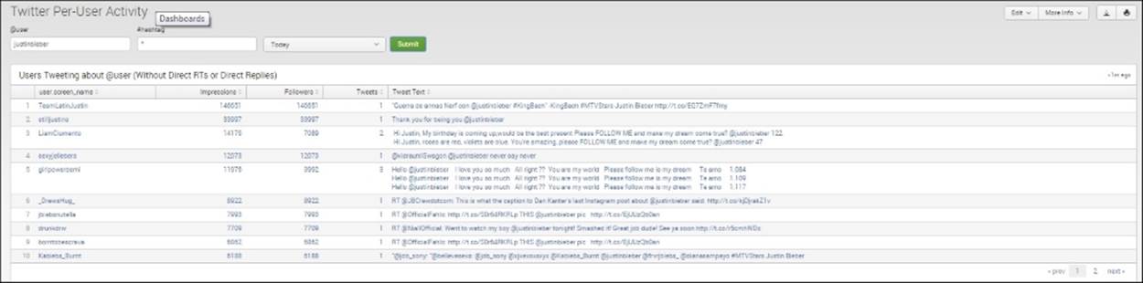
Twitter Per-User Activity for @justinbieber

The search commands used to create this panel are as follows:

index=twitter justinbieber NOT retweeted_status.user.screen_name=justinbieber NOT in_reply_to_screen_name=justinbieber

| fields entities.user_mentions{}.screen_name user.followers_count text user.screen_name

| rename entities.user_mentions{}.screen_name as mentions

| mvexpand mentions

| search mentions=justinbieber

| stats sum(user.followers_count) as Impressions max(user.followers_count) as Followers count as Tweets values(text) as "Tweet Text" by user.screen_name

| sort 20 –Impressions

We won't go through this search string in detail. But basically, the preceding commands look for a username that is not a retweet or used in a reply, and then list them. An agent for a celebrity, or a social media or PR specialist for a company, would be interested in this type of analysis.

Second panel – Users Replying to @user

The following screenshot shows counts for Impressions, Followers, Tweets, and Tweet Text for @user:

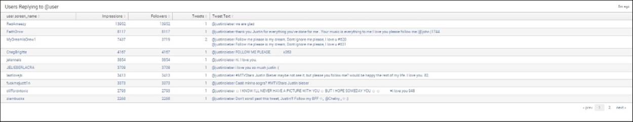
Counts for Impressions, Followers, Tweets, and Tweet Text for @user

The code for creating this panel is as follows:

index=twitter justinbieber in_reply_to_screen_name=justinbieber

| fields entities.user_mentions{}.screen_name user.followers_count text user.screen_name

| rename entities.user_mentions{}.screen_name as mentions | mvexpand mentions

| search mentions=justinbieber

| stats sum(user.followers_count) as Impressions max(user.followers_count) as Followers count as Tweets values(text) as "Tweet Text" by user.screen_name

| sort 20 –Impressions

This panel looks at the top 20 user.screen_names that tweeted @justinbieber during this time period, and then lists the sum of the followers who saw each tweet (renamed Impressions) as well as the number of followers. (Notice that user MyDreamisDrew1 tweeted twice, so the impressions are double the size of the Followers.)

Third panel – Users Retweeting @user

In the following screenshot, we see counts for Impressions, Followers, Tweets, and Tweet Text for users retweeting @user:

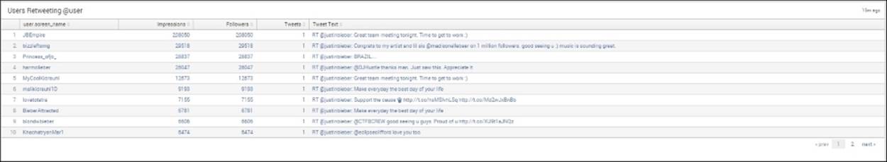
Counts for Impressions, Followers, Tweets and Tweet Text for users retweeting @user

The code used here is as follows:

index=twitter retweeted_status.user.screen_name=justinbieber

| stats sum(user.followers_count) as Impressions max(user.followers_count) as Followers count as Tweets values(text) as "Tweet Text" by user.screen_name

| sort 20 –Impressions

This panel takes those who retweeted a tweet containing @justinbieber, then creates the Impressions and Followers fields and shows them, and then lists those tweets in descending order.

Fourth panel – Users Tweeting about #hashtag

In the fourth panel, we see Impressions, Followers, Tweets, and Tweet Text for users tweeting about #hashtag:

Impressions, Followers, Tweets, and Tweet Text for users tweeting about #hashtag

The code used here is as follows:

index=twitter justinbieber in_reply_to_screen_name=justinbieber

| fields entities.user_mentions{}.screen_name user.followers_count text user.screen_name

| rename entities.user_mentions{}.screen_name as mentions | mvexpand mentions |

search mentions=justinbieber

| stats sum(user.followers_count) as Impressions max(user.followers_count) as Followers count as Tweets values(text) as "Tweet Text" by user.screen_name

| sort 20 –Impressions

This shows the screen_names of the people tweeting in reply to a tweet with @justinbieber that use a hashtag, then shows the impressions and the followers for each, the number of times they tweeted (during this time period), and the actual tweet text. The table is sorted by the number of impressions (descending).

Creating dashboard panels with Twitter data

In the previous section, we shown and described examples of how dashboard panels can be made using Twitter data. Before ending this chapter, we present two additional examples.

Monitoring your hashtag

You might be interested in seeing what kind of traffic a hashtag was getting at a particular time. This could be to follow what people were saying about your company or a public figure. The search code to do this is presented here, for a hashtag of your choice, indicated here by my_hashtag:

index=twitter

| rename entities.hashtags{}.text as hashtags

| fields hashtags

| mvexpand hashtags

| where like(hashtags,"my_hashtag")

| timechart count span=10d

Let's look at this code carefully. We show each pipe on a separate line, just to be clear. We'll start with line 2, where we rename each instance of the text of the hashtag entity as hashtags. In line 3, we limit our pool of data to the field hashtags. In line 4, we use themvexpand command to separate the hashtag field into multiple values, as we have seen before. Then we look for a specific hashtag, which is given in quotes. Here, we have used gameinsight in place of my_hashtag, which was a popular hashtag at the time this book was written. We then use the timechart command to find the count of hashtags during the last 10 days:

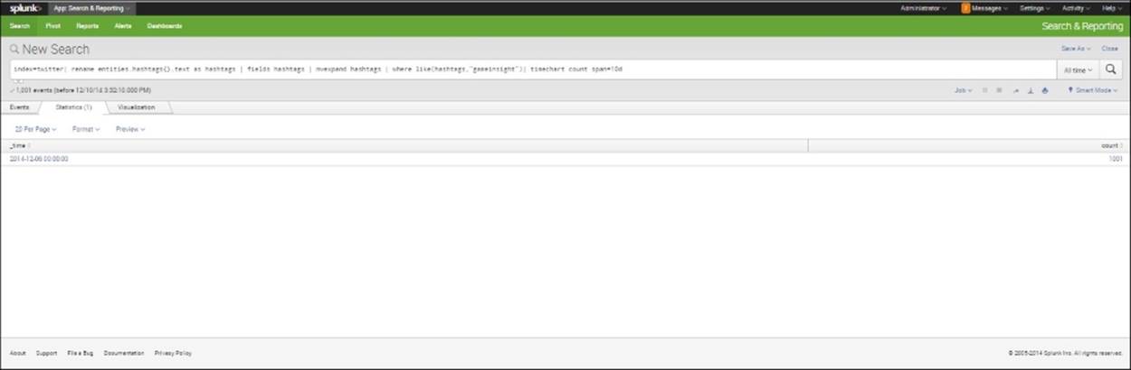
This Search string counts the number of times "gameinsight" appeared

Creating an alphabetical list of screen names for a hashtag

It might be that you are interested in looking at exactly who is tweeting a particular hashtag and precisely what they are saying. To do this, you can use the following code, replacing gameinsight with the hashtag of your choice:

index=twitter

| rename entities.hashtags{}.text as hashtags

| rename user.screen_name as screenname

| fields screenname, hashtags, text

| mvexpand hashtags

| where like(hashtags, "gameinsight")

| table screenname, text

| sort screenname

Going through this code, you can see that we have taken the user.screen_name and renamed it screenname, then limited our data to screenname, hashtags, and text. In the fourth line, we go on to expand the hashtags into multivalued fields. Then we limit our hashtags to those including gameinsight. Finally, we create a table showing the screenname and the text of the tweets, which is in alphabetical order by screenname. This way, we can see who is saying what regarding a particular hashtag. Given the increasing importance of one's image on social media, this type of analysis, as well as the others discussed in this chapter, can be extremely useful.

Summary

In this chapter, we have used the app for Twitter data to learn about how to input live data streams. We have explored in detail the built-in dashboards that come with this app, and have learned about the commands behind each panel and how they work in Splunk. We have also learned more about doing more detailed searches in Splunk. And we have additionally learned about how to use a lookup table to aid our searches.

In the next chapter, we will go on to learn the useful skill of using Splunk to create alerts.