HP Vertica Essentials (2014)

Chapter 5. Performance Improvement

A lot has always been discussed on database performance improvement techniques. In Vertica, because there is no concept of indexes, a major thrust for performance improvement lies upon the concept of projections. Apart from projections, this chapter will also discuss the storage models present in Vertica.

Understanding projections

Traditional databases use row-store architecture. To process a query, a row store reads all of the columns in all of the tables mentioned in the query, regardless of the number of columns a table has. Often, analytical queries access (or require to access) only few columns of a table containing up to several hundred columns, thus making a whole-column-scan unwarranted. Additionally, a whole-column-scan also results in the retrieval of a lot of unnecessary data. Unlike other RDBMSes, Vertica reads the columns from database objects called projections. Consider the following example:

Now, suppose we have the following query:

SELECT A, D, E

FROM Table1 JOIN Table2

ON Table1.C_pk = Table2.C_fk;

On execution of the preceding query, a row store will typically scan through all columns of each table from physical storage, while a column store such as Vertica will only read three columns.

Projections constitute the physical schema of Vertica. In Vertica, a table only serves as a logical schema and doesn't occupy any physical space. All data is stored in the form of projections. It should be noted that there can be more than one projection for a table, that is, the same data can be present in multiple projections. Even though data is repeated, projections consume less space than speculated. A minimum of one projection should exist for each table in the database. This makes sense as projections constitute the physical schema in Vertica. Vertica automatically creates a projection as soon as a table is created. This first projection is called a superprojection. A superprojection contains all columns of a table, thus making sure that all SQL queries can be answered. It should be noted that superprojections are a kind of support projection and are generally not very efficient.

Projections can be compared with materialized views (MVs) and indexes. One key difference between projections, MVs, and indexes is that projections are primary storage and there is no underlying table. In contrast, both MV and indexes are secondary storage and there are one or more underlying tables.

In the traditional sense, Vertica has no raw uncompressed base tables, no materialized views, and no indexes. Everything is taken care of by projections. Of course, our logical schema remains the same as with any other database, that is, tables.

Looking into high availability and recovery

The Vertica database is believed to be K-Safe if any K node(s) fail without causing the database to shut down. In a K-Safe cluster, when a failed node recovers, it joins the database cluster again. All data changes made during the time when the node was down are recovered by querying other nodes in the cluster.

In Vertica, the value of K can be 0, 1, or 2. A K-Safe value implies the maximum number of nodes that can be down at a single point in time without affecting the working of a database. So, if a database with K-safety of one (K=1) loses a node, the database will continue to run normally. Similarly, a database with a K-Safe value of 2 (K=2) will ensure that Vertica can run normally if any two nodes fail at any given point of time. For each K-Safe value, there is a minimum number of nodes that is required. The following table illustrates this:

Vertica doesn't officially support values of K greater than 2.

Projections on a cluster can be stored in the following two ways:

· Unsegmented

· Segmented

Comprehending unsegmented projections

These types of projections are not broken and distributed on different nodes, but rather a copy of the entire projection is maintained on each node, that is, data is replicated across the nodes. It is suggested that small dimensional tables should remain unsegmented. The following illustration shows two projections: Projection 1 and Projection 2. These are replicated across a three-node cluster but unsegmented:

Comprehending segmented projections

In segmented projections, a projection is broken into chunks or segments, and a copy of these segments is maintained on different nodes of the cluster. These replicated projections are known as buddy projections. These projections are recommended for fact tables and dimensional tables with a large amount of data. Consider an example where there is a cluster of three nodes and there is a projection, Proj 1, that needs to be segmented. In order to maintain data on each node, we will need to create two more copies of data: Proj 1 BP1 and Proj 1 BP2. Each of these projections, that is, Proj 1, Proj 1 BP1, and Proj 1 BP2, will be broken into three equal parts and distributed on different nodes. The following example illustrates this more clearly:

Creating projections using Database Designer

Vertica provides a UI-based tool known as Database Designer, which recommends projections on the basis of queries. The following information should be given to Database Designer to create the best projections:

· A set of queries to be run or something similar

· A K-Safe level

· The database should already have tables ready with sample data (not more than 10 GB)

The following are the steps to work on Database Designer:

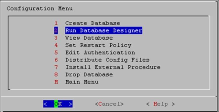
1. We can start Database Designer by navigating to Configuration Menu | Run Database Designer from the admin tools menu, as shown in the following screenshot:

2. Select a database for the design, as illustrated in the following screenshot:

3. Enter the directory where the output of Database Designer will be stored, as shown in the following screenshot:

4. Then, enter the design name, as shown in the following screenshot:

5. The preceding steps were generic. From now, the process forks as per the design type we select:

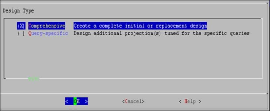
There are two types of designs:

· Comprehensive design

· Query-specific design

The comprehensive design

Comprehensive design lets us design projections for all the tables in the specified schemas. It is suggested to create a comprehensive design when we create a new database, but a comprehensive design for an existing database can also be created if the entire database is not performing up to the mark.

The following are the options for Comprehensive design that will help to control the design in a better fashion:

· Optimize with queries: This option lets us supply queries that will be taken into consideration by Database Designer for the design.

· Update statistics: When this option is selected, the statistics are collected and refreshed. Like any other database technology, precise statistics help Database Designer enhance the compression and query performance.

· Deploy design: When this option is selected, Database Designer deploys the new database design to our database automatically. Although Database Designer saves the SQL script for the new design (projections) in the design location, if needed, we can review the scripts and deploy them manually later.

The following screenshot shows the afore mentioned options:

The query-specific design

Sometimes, we just need to optimize the performance of certain queries. For this purpose, a query-specific design can be employed. It should be noted that a query-specific design will limit design suggestions to the queries we supply. Projections thus created/suggested may hamper, although rarely, the performance of other queries.

The query-specific design process lets us specify the following options:

· Update statistics: When this option is selected, the statistics are collected and refreshed. Like any other database technology, precise statistics help Database Designer enhance the compression and query performance.

· Deploy design: This option installs the new database design. In the process, new projections are added to the database. Later, these projections are populated with data. It should be noted that none of the existing projections are affected by the deployment of a new projection in this process.

The following screenshot shows the afore mentioned options:

If we wish to select the Comprehensive design with the Optimize with queries option or the Query-specific design, then we need to provide a set of queries, as shown in the following screenshot:

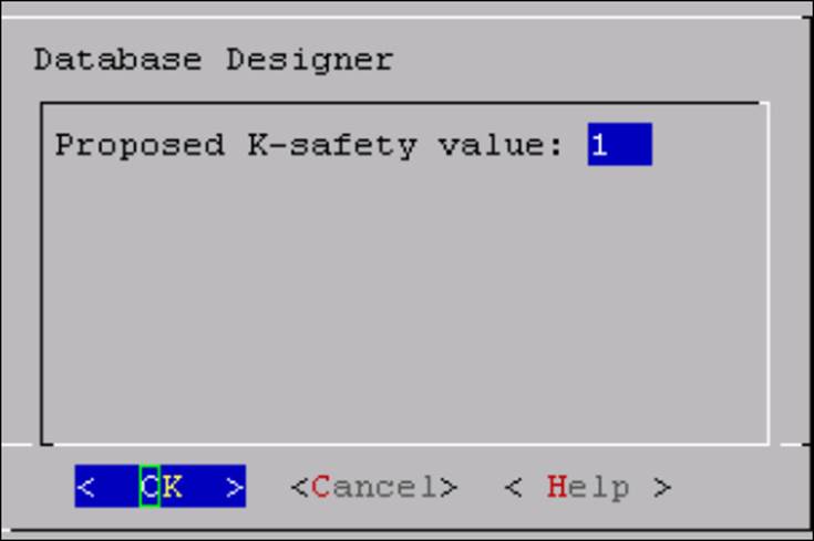
After this, just provide the K-Safe value to start the process, as shown in the following screenshot:

Creating projections manually

If the projection created by Database Designer doesn't meet our needs, then we can write custom projections. Vertica uses the CREATE PROJECTION command to create projections. The following is an example:

CREATE Projection Projection1

(

col1 ENCODING RLE,

col2,

col3 // Column List and Encodings

) AS

SELECT

t1.col1, // Base table query

t1.col2,

t2.col1

FROM table1 t1

INNER JOIN table2 t2 on t1.col1 = t2.col1

ORDER BY t1.col1

SEGMENT BY HASH (t1.col1) ALL NODES OFFSET 1; //Segmentation clause

Column list and encoding

The column list and encoding lists every column within the projection corresponding to the base query (described later in this section) and defines the encoding for each column. For Vertica, it is advisable to use data encoding as it results in fewer disk I/O.

The base query

The base query identifies all of the columns to incorporate in a particular projection. Base queries are just like standard SQL queries with the exception that a base query for large table projections can contain only PK/FK joins from smaller tables.

The sort order

Presorted projections are one of the key ingredients for high-performance queries. We can also optimize a query by matching the projection's sort order to the query's GROUP BY clause. Database Designer does not optimize for GROUP BY queries. Using the GROUP BYpipeline optimization might defeat other optimizations based on the predicate, especially if the predicate is very selective. Therefore, it is suggested not to use it or use it only when exclusively required. So, as a tip, when predicates are not very selective or they are absent, GROUP BY can be used in projections.

Segmentation

As discussed earlier, the SEGMENTATION clause will tell a database to keep projections in a segmented or unsegmented manner.

Segmentation maximizes database performance by distributing the load. It is advisable to use SEGMENT BY HASH to segment large table projections.

For small tables, it is better to keep data unsegmented or non-partitioned. The UNSEGMENT keyword will direct Vertica to do the same. Hence, data will just be replicated and not partitioned nor segmented.

Keeping K-safety (K-Safe) in mind

We can replicate data on all nodes using the UNSEGMENTED ALL NODES keyword. This will ensure high availability and fault tolerance. For large tables, it is imperative to segment corresponding projections. In order to make segmented data fault tolerant and highly available or K-Safe, we need to do the following:

· Create a segmented projection for each fact and large dimension table.

· Create segmented buddy projections for each of the projections. The total number of projections in a buddy set must be two (2) for a K=1 database or three (3) for a K=2 database.

Creating buddy projections

To create a buddy projection, copy the script of the original projection and modify it as follows:

1. Rename it to something similar to the name of the original projection. For example, a projection named retail_sales_fact_P1 could have buddies named retail_sales_fact_P1_B1 and retail_sales_fact_P1_B2.

2. Modify the sort order, if needed.

3. Create an offset to store the segments for the buddy on different nodes. For example, the first buddy in a projection set would have an offset of one (OFFSET 1;), the second buddy in a projection set would have an offset of two (OFFSET 2;), and so on.

A note on table partitioning

Vertica supports data partitioning at a table level, which divides one large table into smaller pieces. The partition remains exclusive to a table and applies to all projections of a given table. In Vertica, tables just form a logical entity and not a physical one; hence, a table partition is also a logical entity. This should not be confused with the segmentation of projections as the latter works at a physical level.

A common use for partitions is to split a table by time periods. For instance, in a table that contains decades of data, we can partition by year or by month. Partitions can improve parallelism during query execution and also enable some optimizations that can improve query performance, at the same time decreasing the deletion time.

Understanding the storage model in Vertica

In order to cater to a wide array of tasks such as DML, bulk loading, and querying, Vertica implements a storage model as shown in the following illustration. This model is the same on each Vertica node.

The Read Optimized Store (ROS) resides on a physical disk storage structure and is organized by projection. Compression is employed at the ROS level to ensure that the disk space occupied by projections is minimal.

Unlike the ROS, the Write Optimized Store (WOS) resides on primary memory, again organized by projection. The WOS stores and sorts the data by epoch. It doesn't compress the data at this level, ensuring high speed writes.

To learn more on how we can control data writing to WOS and ROS, refer to the Bulk Loading section.

Tuple Mover (TM) is a Vertica background process, which is responsible for moving data from primary memory (WOS) to physical disk (ROS). Apart from that, TM is also responsible for removing deleted data and coalescing small ROS containers.

Tuple Mover operations

Tuple Mover performs the following two operations:

· Moveout

· Mergeout

Each data node is responsible for running its own TM tasks, that is, Moveout and Mergeout at its own interval of time.

Moveout

Moveout is responsible for moving data from primary memory (WOS) to physical disk (ROS). Every time a Moveout operation is performed, a new ROS container is created. In the case of COPY…DIRECT (refer Chapter 6, Bulk Loading), new ROS containers are formed. An ROS container is nothing but a set of rows of a projection stored in a group of files. An ROS container contains data pertaining to a single table partition only; however, a table partition can be present in multiple ROS containers. The STORAGE_CONTAINERS system table stores all information regarding the execution of Moveout, as shown:

km=> select * from storage_containers;

-[ RECORD 1 ]-------+-------------------------

node_name | v_km_node0001

schema_name | public

projection_id | 45035996273716454

projection_name | timedata_b1

storage_type | ROS

storage_oid | 45035996273716511

total_row_count | 931

deleted_row_count | 0

used_bytes | 5095

start_epoch | 6

end_epoch | 6

grouping | PROJECTION

segment_lower_bound | 2863311530

segment_upper_bound | 4294967294

-[ RECORD 2 ]-------+-------------------------

node_name | v_km_node0001

schema_name | public

projection_id | 45035996273716440

projection_name | timedata_b0

storage_type | ROS

storage_oid | 45035996273716531

total_row_count | 945

deleted_row_count | 0

used_bytes | 5106

start_epoch | 6

end_epoch | 6

grouping | PROJECTION

segment_lower_bound | 4294967295

segment_upper_bound | 1431655764

Mergeout

A Mergeout operation works at the ROS level and is responsible for removing deleted data and coalescing small ROS containers. When an increased number of ROS containers hinders the performance, Tuple Mover automatically performs a Mergeout operation.

Tuning Tuple Mover

We can tune and tweak certain parameters to control Tuple Mover as per our need. The following table illustrates various configurable parameters for Tuple Mover:

Adding storage locations

It is imperative to add additional storage locations (read directories) as the size of the database grows. Moreover, we can keep crucial files on a high performance physical memory, such as flash drives, in order to boost performance. The following are the points that should be kept in mind before adding an extra storage location:

· Catalog and Data directories should be different.

· Catalog and Data directories should not be shared among nodes.

· A new directory is empty and Vertica has all its rights.

We can check for existing data storages for the whole cluster by running the following query:

SELECT * from V_MONITOR.DISK_STORAGE;

Before adding storage locations, we should decide what type of information we wish to store in this new location. It can be one of the following:

· Any kind of data (projections): DATA.

· Temporary files produced as a by-product of certain database processes: TEMP.

· Both data and temp files. This is the default option: DATA, TEMP.

· We can create locations specific for a non-admin user. It will only store data: USER.

Adding a new location

The ADD_LOCATION() function is used as a query to initialize the new data directory, the node (optional), and the type of information to be stored. The following is an example of this function:

SELECT ADD_LOCATION ('/newLocation/data/', 'v_test_node0003', 'TEMP');

Measuring location performance

We can use MEASURE_LOCATION_PERFORMANCE() to measure the performance of a storage location. This function has the following prerequisites:

· The storage path must be configured for the database.

· Free physical memory greater than or equal to double the RAM on the node. For example, if we have 4 GB of RAM, then the function requires 8 GB of free disk space.

Use the system table DISK_STORAGE to obtain information about disk storage on each database node. The following example measures the performance of a storage location on node2:

=>select measure_location_performance('/ilabs/data/vertica/data/test/v_test_node0001_data','v_test_node0001');

WARNING 3914: measure_location_performance can take a long time to execute. Please check logs for progress

MEasure_location_performance

------------------------------------------------

Throughput : 38 MB/sec. Latency : 51 seeks/sec

(1 row)

The number generated represents the time taken by Vertica to read and write 1 MB of data from the disk, which equates to the following:

IO time = time to read/write 1MB + time to seek = 1/throughput + 1/Latency

In the preceding command, the following is observed:

· Throughput is the average throughput of sequential reads/writes (units in MB per second)

· Latency is for random reads only in seeks (units in seeks per second)

Setting location performance

Additionally, we can set the performance of a location. Setting location performance can really boost the overall database performance as Vertica selectively stores sorted columns (in order) to faster locations of a projection and the rest of the columns to a slower location. To set the performance for a location, a superuser can use the SET_LOCATION_PERFORMANCE() function, as shown:

=> SELECT SET_LOCATION_PERFORMANCE(v_test_node0001','/data/vertica/data/test/v_test_node0001_data','38','51');

In the preceding command, the following is observed:

· '38' is the throughput in MB/second

· '51' is the latency in seeks/second

Understanding storage location tweaking functions

In this section, we will understand how to tweak storage locations with the help of some functions.

Altering

We can use the ALTER_LOCATION_USE() function to modify existing storage locations. This following example alters the storage location on v_test_node0003 to store data only:

=> SELECT ALTER_LOCATION_USE ('/newLocation/data/', 'v_test_node0003', 'DATA');

Dropping

We can use the DROP_LOCATION() function to drop a location. The following example drops a storage location on v_test_node0003 that was used to store temp files:

=> SELECT DROP_LOCATION('/newLocation/data/' , 'v_test_node0003');

The existing data will be merged out either manually or automatically.

Retiring storage locations

To retire a storage location, use the RETIRE_LOCATION() function. The following example retires a storage location on v_test_node0003:

=> SELECT RETIRE_LOCATION('/newLocation/data/' , 'v_test_node0003');

Retiring is different from dropping as in the former case Vertica ceases to store data or temp files to it. Before retiring a location, we must make sure that at least one other location on the node exists to store data and temp files.

Restoring retired storage locations

To restore an already retired location, we can use the RESTORE_LOCATION() function. The following example restores a retired storage location on v_test_node0003:

=> SELECT RESTORE_LOCATION('/newLocation/data/' , 'v_test_node0003');

Summary

In Vertica, projections are the single most important topic that can help in improving performance of a Vertica deployment. As mentioned earlier, it is best to create projections using Database Designer. In the last and final chapter, we will discuss bulk loading of data in Vertica.