Biologically Inspired Computer Vision (2015)

Part IV
Applications

Chapter 16
Nightvision Based on a Biological Model

Magnus Oskarsson, Henrik Malm and Eric Warrant

16.1 Introduction

The quest to understand the biological principles that exquisitely adapt organisms to their environments and that allow them to solve complex problems, has led to unexpected insights into how similar problems can be solved technologically. These biological principles often turn out to be refreshingly simple, even “ingenious,” seen from a human perspective, making them readily transferable to man-made devices. This mimicry of biology – known more broadly as “biomimetics” – has already led to a great number of technological innovations, from Velcro (inspired by the adhesive properties of burdock seed capsules) to convection-based air conditioning systems in skyscrapers (inspired by the nest ventilation system of the African fungus-growing termite). In this chapter, we describe a recent biomimetic advance inspired by the visual systems of nocturnal insects.

Constituting the great majority of all known species of animal life on Earth, the insects have conquered almost every imaginable habitat (excluding oceans). And despite having eyes, brains, and nervous systems only a fraction the size of our own, insects rely on vision to find food, to navigate and home, to locate mates, escape predators and migrate to new habitats. Even though insects do not see as sharply as we do, many experience many more colors, can see polarized light, and can clearly distinguish extremely rapid movements. Remarkably, this is even true of nocturnal insects, whose visual world at night is around 100 million times dimmer than that experienced by their day-active relatives. Research over the past 15–20 years – particularly on fast-flying and highly aerodynamic moths and bees and on ball-rolling dung beetles – indicates that nocturnal insects that rely on vision for the tasks of daily life invariably see extremely well (reviewed by Warrant and Dacke in Ref. [1]). We now know, for instance, that nocturnal insects are able to distinguish colors [2, 3], detect faint movements [4], and avoid obstacles during flight by analyzing optic flow patterns [5], to learn visual landmarks [6–8], to orient to the faint polarization pattern produced by the moon [9], and to navigate using the faint stripe of light provided by the Milky Way [10].

To see so well at night, these insects – whose small eyes struggle to capture sufficient light to see – must overcome a number of fundamental physical limitations in order to extract reliable information from what are inherently dim and very noisy visual images. Recent research has revealed that nocturnal insects employ several neural strategies for this purpose. It is these strategies that have provided the inspiration for a new night-vision algorithm that dramatically improves the quality of video recordings made in very dim light.

Most people have experienced problems with taking pictures and recording video under poor lighting conditions. Low contrast and grainy images are often the result. Most of today's digital cameras are based on the same principles that animal eyes are built on. The light that hits the camera is focused by an optical system, typically involving one or many lenses. The light is focused on a sensor that transforms the photon energy into an electrical signal. These sensors are typically CCD or CMOS arrays, arranged in a grid of pixels. The electric current is then transformed into a digital signal that can be stored in memory.

Since the underlying principles of both animal and camera vision are similar, it is natural to try to mimic the neural processes of nocturnal animals in order to construct efficient computer vision algorithms. In the following sections, we describe both the underlying biological principles and our computer vision approach in detail. Parts of the work in this chapter have previously been presented in [11–14].

16.1.1 Related Work

Enhancing low-light video in most cases involves some form of amplification of the signal in order to increase the contrast. This is – as described in the following sections – also true for our approach. This amplification will introduce more apparent noise in the signal, and the most difficult part of the video enhancement process is the reduction of noise in the signal.

There exists a multitude of noise reduction techniques that apply weighted averaging for noise reduction purposes. Many authors have additionally realized the benefit of trying to reduce the noise by filtering the sequences along motion trajectories in spatiotemporal space and in this way, ideally, avoid motion blur and unnecessary amounts of spatial averaging. These noise reduction techniques are usually referred to as motion-compensated (spatio-)temporal filtering. In Ref. [15], means along the motion trajectories are calculated while in Refs [16] and [17], weighted averages, dependent on the intensity structure and noise in a small neighborhood, are applied. In Ref. [18], so-called linear minimum mean square error filtering is used along the trajectories. Most of the motion-compensated methods use somekind of block-matching technique for the motion estimation that usually, for efficiency, employs rather few images, commonly two or three. However, in Refs [16, 18] and [19], variants using optical flow estimators are presented. A drawback of the motion-compensating methods is that the filtering relies on a good motion estimation to give a good output, without excessive blurring. The motion estimation is especially complicated for sequences severely degraded by noise. Different approaches have been applied to deal with this problem, often by simply reducing the influence of the temporal filter in difficult areas. This, however, often leads to disturbing noise at, for example, object contours.

Some of the most successful approaches to image denoising over the recent years belong to the group of block-matching algorithms. These include the nonlocal means algorithms [20] and the popular BM3D approach [21, 22]. BM3D is the algorithm that we have tried which has the most comparable result to our own.

Another class of noise reducing video processing methods uses a cascade of directional filters and in this way analyzes the spatiotemporal intensity structure in the neighborhood of each point. The filtering and smoothing is done primarily in the direction that corresponds to the filter that gives the highest output, cf. Refs [23, 24] and [25]. These methods work well for directions that coincide with the fixed filter directions but have a pronounced degradation in the output in directions in-between the filter directions. For a review of a large number of spatiotemporal noise reduction methods, see Ref. [26].

An interesting family of smoothing techniques for noise reduction are the ones that solve an edge-preserving anisotropic diffusion equation on the images. This approach was pioneered by Perona and Malik [27] and has had many successors, including the work by Weickert [28]. These techniques have also been extended to 3D and spatiotemporal noise reduction in video, cf. Refs [29] and [30]. In Refs [29] and [31], the so-called structure tensor or second-moment matrix is applied in a similar manner to our approach in order to analyze the local spatiotemporal intensity structure and steer the smoothing accordingly. The drawbacks of techniques based on diffusion equations include the fact that the solution has to be found using an often time-consuming iterative procedure. Moreover, it is very difficult to find a suitable stopping time for the diffusion, at least in a general and automatic manner. These drawbacks make these approaches, in many cases, unsuitable for video processing.

A better approach is to apply single-step structure-sensitive adaptive smoothing kernels. The bilateral filters introduced by Tomasi and Manduchi [32] for 2D images falls within this class. Here, edges are maintained by calculating a weighted average at every point using a Gaussian kernel, where the coefficients in the kernel are attenuated on the basis of how different the intensities are in the corresponding pixels compared to the center pixel. Thismakes local smoothing very dependent on the correctness in intensity in the center pixel, which cannot be assumed in images heavily disturbed by noise.

An approach that is closely connected to both bilateral filtering and to anisotropic diffusion techniques based on the structure tensor is the structure-adaptive anisotropic filtering presented by Yang et al. [33]. We base our spatiotemporal smoothing on the ideas in this paper, but extend it to our special setting for video and very low light levels. For a study of the connection between anisotropic diffusion, adaptive smoothing, and bilateral filtering, see Ref. [34].

Another group of algorithms connected to our work are in the field of high dynamic range (HDR) imaging, cf. Ref. [35, 36] and the references therein. The aim of HDR imaging is to alleviate the restriction caused by the low dynamic range of ordinary CCD cameras, that is, the restriction to the ordinary 256 intensity levels for each color channel. Most HDR imaging algorithms are based on using multiple exposures of a scene with different settings for each exposure and then using different approaches for storing and displaying this extended image data. However, the HDR techniques are not especially aimed at the kind of low-light-level data that we are targeting in this work, where the utilized dynamic range in the input data is in the order of 5–20 intensity levels and the SNR is extremely low.

There are surprisingly few published studies that particularly target noise reduction in low-light-level video. Two examples are the method by Bennett and McMillan [37] and the technique presented by Lee et al. [38]. In Ref. [38], very simple operations are combined in a system presumably developed for easy hardware implementation in, for example, mobile phone cameras and other compact digital video cameras; this method cannot handle the high levels of noise that we target in this work. The approach taken by Bennett and McMillan [37] for low-dynamic-range image sequences is more closely connected to our technique. Their virtual exposure framework includes the bilateral ASTA-filter (adaptive spatiotemporal accumulation) and a tone mapping technique. The ASTA-filter, which changes to relatively more spatial filtering in favor of temporal filtering when motion is detected, is in this way related to the biological model described in the following sections. However, as bilateral filters are applied, the filtering is edge sensitive and the temporal bilateral filter is additionally used for local motion detection. The filters apply novel dissimilarity measures to deal with the noise sensitivity of the original bilateral filter formulation. The filter size applied at each point is decided by an initial calculation of a suitable amount of amplification using tone mapping of an isotropically smoothed version of the image. A drawback of the ASTA-filter is that it requires global motion detection as a preprocessing step to be able to deal with moving camera sequences. The sequence is then warped to simulate a static camerasequence.

16.2 Why Is Vision Difficult in Dim Light?

From the outset, it is important to point out that the nocturnal visual world is essentially identical to the diurnal visual world. The contrasts and colors of objects are almost identical. The only real distinguishing difference is the mean level of light intensity, which can be up to 11 orders of magnitude dimmer at night [39, 40], depending on the presence or absence of moonlight and clouds, and whether the habitat is open or closed (i.e., beneath the canopy of a forest). It is this difference that severely limits the ability of a visual system to distinguish the colors and contrasts of the nocturnal world. Indeed, many animals, especially diurnal animals, distinguish very little at all. In the end, the greatest challenge for an eye that views a dimly illuminated object is to absorb sufficient photons of light to reliably discriminate it from other objects [6, 40–42]. The main role of all photoreceptors is to transduce incoming light into an electrical signal whose amplitude is proportional to the light's intensity. The mechanism of transduction involves a complex chain of biochemical events within the photoreceptor that uses the energy of light to open ion channels in the photoreceptor membrane, thereby allowing the passage of charged ions and the generation of an electrical response. Photoreceptors are even able to respond to single photons of light with small but distinct electrical responses known as bumps (as they are called in the invertebrate literature: Figure 16.1a,b). At higher intensities, the bump responses fuse to create a graded response whose duration and amplitude is proportional to the duration and amplitude of the light stimulus. At very low light levels, a light stimulus of constant intensity will be coded as a train of bumps generated in the retina at a particular rate, and at somewhat higher light levels, the constant intensity will be coded by a graded potential of particular amplitude. At the level of the photoreceptors, the reliability of vision is determined by the repeatability of this response: for repeated presentations of the same stimulus, the reliability of vision is maximal if the rate of bump generation, or the amplitude of the graded response, remains exactly the same for each presentation. In practice, this is never the case, especially in dim light.

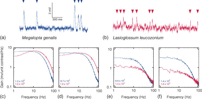
Figure 16.1 Adaptations for nocturnal vision in the photoreceptors of the nocturnal sweat bee Megalopta genalis, as compared to photoreceptors in the closely related diurnal sweat bee Lasioglossum leucozonium. (a) and (b) Responses to single photons (or “photon bumps”: arrowheads) recorded from photoreceptors in Megalopta (a) and Lasioglossum (b) Note that the bump amplitude is larger, and the bump time course much slower, in Megalopta than in Lasioglossum. (c) – (f) Average contrast gain as a function of temporal frequency in Megalopta (blue curves, cells) and Lasioglossum (red curves, cells) at different adapting intensities, indicated as “effective photons” per second in each panel for each species (for each species, each stimulus intensity was calibrated in terms of “effective photons,” i.e., the number of photon bumps per second the light source elicited, thereby eliminating the effects of differences in the light gathering capacity of the optics between the two species, which is about 27: Ref. [43]). In light-adapted conditions (c) and (d), both species reach the same maximum contrast gain per unit bandwidth, although Lasioglossum has broader bandwidth and a higher corner frequency (the frequency at which the gain has fallen off to 50% of its maximum). In dark-adapted conditions (e) and (f), Megalopta has a much higher contrast gain per unit bandwidth. All panels adapted with kind permission from Ref. [44].

Why is this so? The basic answer is that the visual response (and as a consequence, its repeatability) is degraded by visual “noise.” Part of this noise arises from the stochastic nature of photon arrival and absorption (governed by Poisson statistics): each sample of absorbed photons (or signal) has a certain degree of uncertainty (or noise) associated with ( photons). The relative magnitude of this uncertainty (i.e., ) is greater at lower rates of photon absorption, and these quantum fluctuations set an upper limit to the visual signal-to-noise ratio [45–47]. As light levels fall, fewer photons are absorbed, the noise relative to the signal is greater, and less of it can be seen. This photon “shot noise” limits detection reliability and is equally problematic for artificial imaging systems, such as cameras, as it is for eyes.

There are also two other sources of noise that further degrade visual discrimination by photoreceptors in dim light. The first of these, referred to as “transducer noise,” arises because photoreceptors are incapable of producing an identical electrical response, of fixed amplitude, latency, and duration, to each (identical) photon of absorbed light. This source of noise, originating in the biochemical processes leading to signal amplification, degrades the reliability of vision, particularly at slightly brighter light levels when photon shot noise no longer dominates [43, 48, 49].

The second source of noise, referred to as “dark noise,” arises because of the occasional thermal activation of the biochemical pathways responsible for transduction, which even occur in perfect darkness [50]. These activations produce “dark events,” electrical responses that are indistinguishable from those produced by real photons, and these are more frequent at higher retinal temperatures. At very low light levels this dark noise can significantly contaminate visual signals. In insects and crustaceans, dark events seem to be rare, only around 10 every hour at , at least in those species where it has been investigated [43, 51, 52]. But in nocturnal toad rods, the rate is much higher – 360 per hour at [53] – and this sets the ultimate limit to visual sensitivity [54, 55].

16.3 Why Is Digital Imaging Difficult in Dim Light?

As discussed in the introduction, animal eyes and digital cameras share much of their underlying functions, from the optics to the sensor. A digital camera's CCD or CMOS sensor is the corresponding element to the retina and photoreceptors in biology, and the basic purpose is the same – to convert light photons into an electrical signal that can be measured andinterpreted. Many of the noise sources described in the previous section are therefore the same or analogous to the ones found in digital cameras. We now briefly discuss the specific characteristics of different types of noise that are present in digital images and relate them to their biological counterparts. For an excellent review of noise in digital cameras based on CCD sensors, see Ref. [56].

The incoming light to the digital camera, of course, suffers from the same physical limitations as the incoming light to an eye. In addition, as described in the previous section, photon shot noise is particularly problematic at low light levels. The incoming light to a sensor array is converted to an electrical signal by the semiconductor. This signal is amplified on the chip to produce a measurable voltage. The “transducer noise” found in photoreceptors has its technical counterparts in “fixed pattern noise,” “blooming,” and “read noise.” Fixed pattern noise is, as its name indicates, a variation in response of different spatial pixels to uniform illumination (due to variations in quantum efficiency and charge collection volume). Blooming is the process when the illumination of nearby pixels influences a pixel's own response. This effect can in many cases be ignored. The read noise is generated by the amplification at each pixel. It can often be modeled as zero, that is, noise that is independent of the number of collected electrons. This noise dominates shot noise at low signal levels.

In the previous section, the “dark noise” in photoreceptors was described. This thermal effect is also present in digital sensors and is called dark current noise. Thermal energy generates free electrons in silicon and this will generate signals that are indistinguishable from the true signal. The effect of dark current noise is more severe at higher temperatures.

Finally, in order to produce a digital image, the electrical signal is quantized into a digital signal with a fixed number of bits. Depending on the chosen bit depth, this process can influence the output more or less, but it is often reasonable to model it as an addition of a zero mean, uniformly distributed, noise term.

From this discussion, it is clear that animals have to address many of the same noise issues as we have in digital cameras. This is especially true at low light levels.

16.4 Solving the Problem of Imaging in Dim Light

As we have seen above, the paucity of photons in dim light causes fundamental limitations to imaging reliability in both eyes and cameras. We next describe how these limitations can be overcome in visual systems, by describing the neural adaptations that have evolved for improving visual reliability in dim light. The adaptations that have evolved over millions of years of evolution are surprisingly elegant and simple and essentially involve two main processing steps: (i) an enhancement of the neural image created in the retina and (ii) a subsequent optimal filtering of this image in space and time at a higher level in the visual system. These two processing steps are the ones we have now employed in the development of a new night-vision algorithm that dramatically improves the quality of video recordings made in very dim light.

We now give an overview of the basic steps in our algorithm. The details of the different steps and their biological motivations are given in the subsequent sections. We start with a low-light video sequence , where is a spatiotemporal point or voxel. One frame of an example low-light sequence is given in Figure 16.2 (a). The first step in our algorithm is the amplification of the signal. This is done by applying a one-dimensional nonlinear amplification function on the input gray values (or color values) so that . The function could be fixed or adapted to the input values. Some examples are discussed in Section 16.4.1. Since we not only amplify the signal but also the noise, we obtain in general a very noisy output video sequence. One frame of an amplified sequence is given in Figure 16.2 (b). Now comes the difficult part, namely, to reduce the noise but keep the signal intact. In order to do this we must in some way distinguish the noise from the signal.

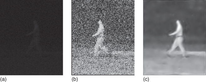
Figure 16.2 (a) One frame from a very dark input sequence. We have little contrast in the image and the details are hard to discern. (b) One frame of the amplified sequence. Here we have structures clearly visible, but the noise in the image has also been amplified. (c) One frame from the final output of Algorithm 16.1. The structures are preserved and the noise has been highly suppressed.

We try to mimic the ideas from the summation principles found in nocturnal insects, where the signal is retrieved through summing in space and time. The details are described in Section 16.4.2.

Almost all noise reduction algorithms are based on averaging the signal. But we do not want to average pixels or voxels that have different signal value, that is, we do not want to average over edges in the signal structure. Since we are dealing with a video sequence, edges appear for two different reasons, (i) due to differences in physical appearance of objects, such as boundaries of objects or texture and color changes and (ii) due to motion of either the camera or objects.

We consider the image sequence as a spatiotemporal volume, as depicted to the left in Figure 16.3. Our goal is to construct smoothing summation kernels that adapt to the local spatiotemporal intensity structure. These kernels should be large in directions where there are no edges and small in directions where we have strong edges. To the right in Figure 16.3 the kernels for two different points are shown. The man walking gives rise to an intensity streak in the image stack. The estimated kernels adapt to this local spatiotemporal structure so that we do not get smoothing over edges. Notice that the kernel at the point with a more structurally isotropic neighborhood is quite isotropic, whereas the kernel at the point with the man walking is elongated in the direction of the intensity streak.

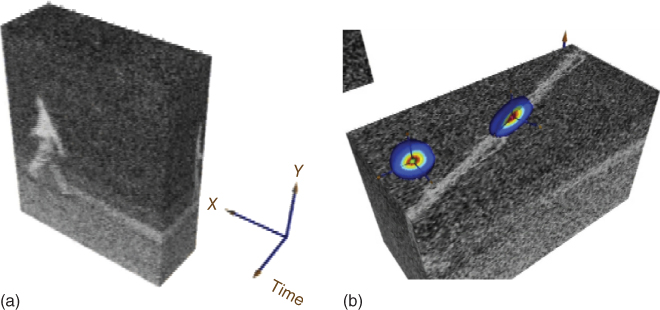
Figure 16.3 This figure illustrates the image stack and the smoothing kernel construction for the image sequence in Figure 16.2. (a) The image stack with the corresponding coordinate system. (b) We have cut the stack at a fixed -coordinate and superimposed the kernels at two different points. The man walking gives rise to an intensity streak in the image stack. The estimated kernels adapt to this local spatiotemporal structure so that we do not get smoothing over edges. Notice that the kernel at the point with the more structurally isotropic neighborhood is quite isotropic, whereas the kernel at the point with the man walking is elongated in the direction of the intensity streak.

We use the so-called structure tensor to estimate the local spatiotemporal structure at each point and use this to construct the smoothing kernels. This will also include calculating the eigenvalues and eigenvectors that we use to orient and stretch our kernels. The details are given in Section 16.4.2.2. When we have constructed the kernels we can estimate the new gray values by integration (or summation as we are dealing with discrete structures). The summation is done over a local space–time neighborhood for each point , typically voxels. The different steps are summarized in Algorithm 16.1.

16.4.1 Enhancing the Image

In this section, we describe the first step in our method. We start with a biological motivation and then discuss the intensity transformation step in detail.

16.4.1.1 Visual Image Enhancement in the Retina

As we have mentioned previously, most animal photoreceptors are capable of detecting single photons of light, responding to them with small but discrete voltage responses that in insects are known as “bumps” (Figure 16.1(a) and (b)). Research has revealed that these bumps are much larger in nocturnal and crepuscular insects than in diurnal insects [44, 57], revealing an intrinsic benefit for vision in dim light. From electrophysiological recordings of photoreceptors in two closely related nocturnal and diurnal halictid bee species – the nocturnal Megalopta genalis (Figure 16.1(a)) and the diurnal Lasioglossum leucozonium(Figure 16.1(b)) – bump amplitude in the nocturnal species was found to be much greater than in the diurnal species [44]. These larger bumps have also been reported from other nocturnal and crepuscular arthropods (e.g., crane flies, cockroaches, and spiders [57–60]); and in locusts – which are considered to be diurnal insects – bump size can even vary at different times of the day, becoming significantly larger at night [61]. Larger bumps indicate that the photoreceptor's gain of transduction is greater, and thus in Megalopta the gain of transduction is greater than in Lasioglossum. This higher transduction gain manifests itself as a higher “contrast gain,” which means that the photoreceptor has a greater voltage response per unit change in light intensity (or contrast). At lower light levels, the contrast gain is up to five times higher in Megalopta than in Lasioglossum, which results in greater signal amplification and the potential for improved visual reliability in dim light (Figure 16.1(c)–(f)). One problem with having a higher gain is that it not only elevates the visual signal it also elevates several sources of visual noise by the same amount. Thus, for this strategy to pay off, subsequent stages of processing are needed to reduce the noise. As we will see in the following, this processing involves a summation of photoreceptor responses in space and time.

Algorithm 1: Low-Light Video Enhancement

1. 1: Given a low-intensity input video sequence:

2. 2: Apply an amplifying intensity transformation ,

3. 3: for each and a neighborhood

4. 4: Calculate the structure tensor .

5. 5: Calculate the eigenvalues and eigenvectors of .

6. 6: Construct the summation kernel ,

7. 7: Integrate the output intensity:

8. 8: end for

In addition to a higher contrast gain, the photoreceptors of nocturnal insects tend also to be significantly slower than those of their day-active relatives. Despite compromising temporal resolution, slower vision in dim light (analogous to having a longer exposure time on a camera) is beneficial because it increases the visual signal-to-noise ratio and improves contrast discrimination at lower temporal frequencies by suppressing photon noise at frequencies that are too high to be reliably resolved [64, 65]. Temporal resolution can be measured in several ways, for instance, by measuring the ability of a photoreceptor to follow a light source whose intensity modulates sinusoidally over time: a photoreceptor that can follow a light source modulating at a high frequency is considered to be fast. Thus, in the frequency domain, slower vision is equivalent to saying that the temporal bandwidth is narrow, or more precisely, that the temporal corner frequency is low – this is often defined as the frequency where the response has fallen to 50% of its maximum value (i.e., by 3 dB), and lower values indicate slower vision. In Megalopta it is around 7 Hz in dark-adapted conditions. In diurnal Lasioglossum the dark-adapted corner frequency is nearly three times the value found in Megalopta, around 20 Hz, a value that is nonetheless considerably less than that typical of the diurnal, highly maneuverable and rapidly flying higher flies (50–107 Hz; [57]). The difference in temporal properties between the two bee species are most likely due to different photoreceptor sizes, and different numbers and types of ion channels in the photoreceptor membrane [57, 66–69].

16.4.1.2 Digital Image Enhancement

The procedure of intensity transformation is also commonly referred to as tone mapping. Tone mapping could actually be performed either before or after the noise reduction, with a similar output, as long as the parameters for the smoothing kernels are chosen to fit the current noise level.

In the virtual exposures method of Bennett and McMillan [37], a tone mapping procedure is applied where the actual mapping is a logarithmic function similar to the one proposed by Drago et al. [70]. The tone mapping procedure also contains additional smoothing using spatial and temporal bilateral filters and an attenuation of details, found by the subtraction of a filtered image from a nonfiltered image. We instead choose to do all smoothing in the separate noise reduction stage and here concentrate on the tone mapping.

The tone-mapping procedure of Bennett and McMillan involves several parameters, both for the bilateral smoothing filters and for changing the acuteness of two different mapping functions – one for the large-scale data and one for the attenuation of the details. These parameters have to be set manually and will not adapt if the lighting conditions change in the image sequence. Since we aim for an automatic procedure we instead opt for a modified version of the well-known procedure of histogram equalization, cf. Ref. [71]. Histogram equalization is parameter-free and increases the contrast in an image by finding a tone mapping that evens out the intensity histogram of the input image as much as possible. In short, histogram equalization works in the following way. We assume that we have an input image and an output image , both defined with continuous gray values , and where the gray value distribution of is . The output image is obtained by transforming the input image with a gray level transformation so that the output distribution is flat, that is, with the distribution . If we further assume that is an increasing function, with and the following equation will hold:

16.1

So by applying the transformation

16.2

we get an output image with a completely flat distribution. This derivation works exactly for continuous images, but as real images are discrete, the integration is replaced by a summation of the discrete histogram of the input image and the resulting image only has an approximately flat distribution. Furthermore, for many images, histogram equalization gives a too extreme mapping, which, for example, saturates the brightest intensities so that structure information here is lost. It also heavily changes the local intensity distribution in ways that change the appearance of the images. We therefore apply contrast-limited histogram equalization as presented by Pizer et al. in Ref. [72], but without the tiling that applies different mappings to different areas (tiles) in the image. In the contrast-limited histogram equalization, a parameter, the clip-limit , sets a limit on the derivative of the slope of the mapping function. If the mapping function, found by histogram equalization exceeds this limit, the increase in the critical areas is spread equally over the mapping function. An example can be seen in Figure 16.2 (b). As illustrated in the image, this process amplifies the signal, but just as in the biological system from the previous section, it is clear that we need to address the amplified noise in the signal.

16.4.2 Filtering the Image

16.4.2.1 Spatial and Temporal Summation in Higher Visual Processing

As mentioned in Section 16.2, even though slow photoreceptors of high contrast gain are potentially beneficial for improving visual reliability in dim light, these benefits may not be realized because of the contamination of visual signals by various sources of visual noise. The solution to overcome the problems of noise contamination is to neurally sum visual signals in space and time [41, 73–77].

We have already discussed summation of photons in time above: when light gets dim, the slower photoreceptors of nocturnal animals can improve visual reliability by integrating signals over longer periods of time [41, 64, 65]. Even slower vision could be obtained by neurally integrating (summing) signals at a higher level in the visual system. However, temporal summation has a cost: the perception of fast-moving objects is seriously degraded. This is potentially disastrous for a fast-flying nocturnal animal (such as a nocturnal bee or moth) that needs to negotiate obstacles. Not surprisingly, temporal summation is more likely to be employed by slow-moving animals. Summation of visual signals in space can also improve image quality. Instead of each visual channel collecting photons in isolation (as in bright light), the transition to dim light could activate specialized, laterally spreading neurons which couple the channels together into groups. Each of the summed groups – themselves now defining the channels – could collect considerably more photons over a much wider visual angle, albeit with a simultaneous and unavoidable loss of spatial resolution. Despite being much brighter, the image would become necessarily coarser. In Megalopta, such laterally spreading neurons have been found in the first optic ganglion (lamina ganglionaris), the first visual processing station in the brain. The bee's four classes of lamina monopolar cells (or L-fibers, L1–L4) – which are responsible for the analysis of photoreceptor signals arriving from the retina – are housed within each neural “cartridge” of the lamina, a narrow cylinder of lamina tissue that resides below each ommatidium. Compared to the L-fibers of the diurnal honeybee Apis mellifera, those of Megalopta have lateral processes that extensively spread into neighboring cartridges (Figure 16.4(a)): cells L2, L3, and L4 spread to 12, 11, and 17 lamina cartridges respectively, while the homologous cells in Apis spread respectively to only 2, 0, and 4 cartridges [62, 78]. Similar laterally spreading neurons have also been found in other nocturnal insects, including cockroaches [79], fireflies [80], and hawkmoths [81].

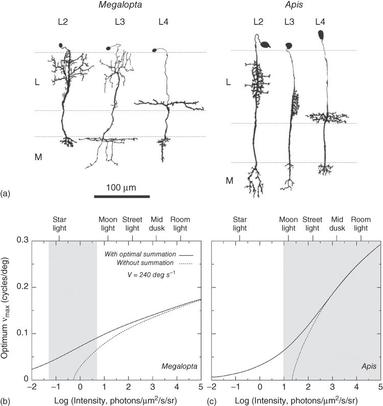
Figure 16.4 Spatial summation in nocturnal bees. (a) Comparison of the first-order interneurons – L-fiber types L2, L3, and L4 – of the Megalopta genalis female (i) and the worker honeybee Apis mellifera (ii). Compared to the worker honeybee, the horizontal branches of L-fibers in the nocturnal halictid bee connect to a much larger number of lamina cartridges, suggesting a possible role in spatial summation. L = lamina, M = medulla. Reconstructions from Golgi-stained frontal sections. Adapted from Refs [62, 63]. (b) and (c) Spatial and temporal summation modeled at different light intensities in Megalopta genalis and (b) Apis mellifera (c) for an image velocity of 240 deg/s (measured from Megalopta genalis during a nocturnal foraging flight [6]). Light intensities are given for 540 nm, the peak in the bee's spectral sensitivity. Equivalent natural intensities are also shown. The finest spatial detail visible to flying bees (as measured by the maximum detectable spatial frequency, ) is plotted as a function of light intensity. When bees sum photons optimally in space and time (solid lines) vision is extended to much lower light intensities (nonzero ) compared to when summation is absent (dashed lines). Note that nocturnal bees can see in dimmer light than honeybees. Gray areas denote the light intensity window within which each species is normally active (although honeybees are also active at intensities higher than those presented on the graph). Figure reproduced from Ref. [40] with permission from Elsevier.

Spatial and temporal summation strategies have the potential to greatly improve the visual signal-to-noiseratio in dim light (and thereby the reliability of vision) for a narrower range of spatial and temporal frequencies [77, 82, 83]. However, despite the consequent loss in spatial and temporal resolution, summation would tend to average out the noise (which is uncorrelated between channels) or significantly reduce its amplitude. Thus, summation would maximize nocturnal visual reliability for the slower and coarser features of the world. Those features that are faster and finer – and inherently noisy – would be filtered out. However, it is, of course, far better to see a slower and coarser world, than nothing at all.

These conclusions can be visualized theoretically [77]. Both Megalopta (Figure 16.4(b)) and Apis (Figure 16.4(c)) are able to resolve spatial details in a scene at much lower intensities with summation than without it [82]. These theoretical results assume that both bees experience an angular velocity during flight of deg/s, a value that has been measured from high-speed films of Megalopta flying at night. At the lower light levels where Megalopta is active, the optimum visual performance shown in Figure 16.4(b) is achieved with an integration time of about 30 ms and summation from about 12 ommatidia (or cartridges). This integration time is close to the photoreceptor's dark-adapted value [6], and the extent of predicted spatial summation is very similar to the number of cartridges to which the L2 and L3 cells actually branch [62], thus strengthening the hypothesis that the lamina monopolar cells are involved in spatial summation. Interestingly, even in the honeybee Apis, summation can improve vision in dim light (Figure 16.4(c)). The Africanized subspecies, Apis mellifera scutellata, and the closely related south-east Asian giant honeybee Apis dorsata, both forage on large pale flowers during dusk and dawn, and even throughout the night, if a moon half-full or larger is present in the sky. This ability can be explained only if bees optimally sum photons over space and time [84], and this is also revealed in Figure 16.4(c) (for an angular velocity of 240 deg/s). At the lower light levels where Apis is active, the optimum visual performance shown in Figure 16.4(c) is achieved with an integration time of about 18 ms and summation from about three or four cartridges. As in Megalopta, this integration time is close to the photoreceptor's dark-adapted value, and the extent of predicted spatial summation is again very similar to the number of cartridges to which the L2 and L3 cells actually branch.

16.4.2.2 Structure Tensor Filtering of Digital Images

We now present our summation method inspired by the biological principles from the previous section. It is in parts based on the structure-adaptive anisotropic image filtering by Yang et al. [33] but in order to improve its applicability to video data and make it suitable for our low-light-level vision objective, it involves a number ofmodifications and extensions.

A new image is obtained, by applying at each spatiotemporal point , a kernel to the original image such that

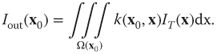
16.3

where

16.4

is a normalizing factor. The normalization makes the sum of the kernel elements equal to in all cases, so that the mean image intensity does not change. The area over which the integration, or in the discrete case, summation, is made is chosen as a finite neighborhood centered around , typically voxels.

Since we want to adapt the filtering to the spatiotemporal intensity structure at each point, in order to reduce blurring over spatial and temporal edges, we calculate a kernel individually for each point . The kernels should be wide in directions of homogeneous intensity and narrow in directions with important structural edges. To find these directions, the intensity structure is analyzed by the so-called structure tensor or second-moment matrix. The structure tensor has been applied in image analysis in numerous papers, for example, Refs [85–87]. The tensor is defined in the following way:

16.5

where

16.6

is the spatiotemporal intensity gradient of at the point . is the Gaussian kernel function

16.7

where is the normalizing factor. The notation means elementwise convolution of the matrix in a neighborhood centered at . It is this convolution that gives us the smoothing in the direction of gradients, which is the key to the noise insensitivity of this method. The numerical estimates of the time derivatives in equation (16.6) are in our implementations taken symmetrically around the given frame for the batch version of our method. We have also implemented an online version where we take the time derivatives only backward from the current frame.

Eigenvalue analysis of will now give us the structural information that we seek. The eigenvector , corresponding to the smallest eigenvalue , will be approximately parallel to the direction of minimum intensity variation while the other two eigenvectors will be orthogonal to this direction. The magnitude of each eigenvalue will be a measure of the amount of intensity variation in the direction of the corresponding eigenvector. For a deeper discussion on eigenvalue analysis of the structure tensor, see Ref. [88].

The basic form of the kernels that are constructed at each point is that of a Gaussian function,

16.8

including a rotation matrix and a scaling matrix . The rotation matrix is constructed from the eigenvectors of ,

16.9

while the scaling matrix has the following form:

16.10

The function is a decreasing function that sets the width of the kernel along each eigenvalue direction. The theory in Ref. [33] is mainly developed for 2Dimages and measures of corner strength and of anisotropism, both involving ratios of the maximum and minimum eigenvalues, are there calculated at every point . An extension of this to the 3D case is then discussed. However, we have not found these two measures to be adequate for the 3D case because they focus too much on singular corner points in the video input and to a large extent disregard the linear and planar structures that we want to preserve in the spatiotemporal space. For example, a dependence of the kernel width in the temporal direction on the eigenvalues corresponding to the spatial directions does not seem appropriate in a static background area. We instead simply let an exponential function depend directly on the eigenvalue in the current eigenvector direction in the following way:

16.11

where , so that attains its maximum below and asymptotically approaches its minimum when . The parameter scales the width function along the -axis and has to be set in relation to the current noise level. Since the part of the noise that stems from the quantum nature of light, that is, the photon shot noise, depends on the brightness level, it is signal-dependent and the parameter should ideally be set locally. However, we have noticed that when the type of camera and the type of tone mapping is fixed, a fixed value of usually works for a large part of the dynamic range. When changing the camera and tone mapping approach, a new value of has to be found for optimal performance.

When the widths have been calculated and the kernel subsequently constructed according to (16.8), Eq. (16.3) is used to calculate the output intensity of the smoothing stage at the current pixel .

In biological vision, edges are often perceived stronger than they actually are. This effect, called lateral inhibition, is due to the ability of an excited neuron to reduce the response of its neighboring neurons. We have mimicked this behavior in an edge-sharpening version of our algorithm. In order to do this, we simply replace the Gaussian kernel with the following base kernel:

16.12

which is stretched and rotated in the same way as before. In the top row of Figure 16.5, the difference between the two kernels is shown. The bottom row shows the output of our algorithm using the two different kernels.

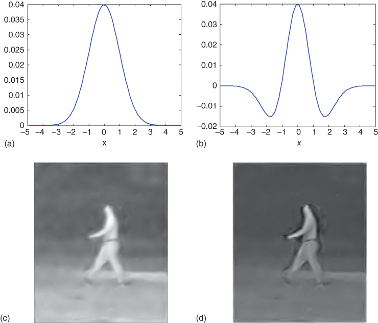
Figure 16.5 This shows the impact of using the lateral inhibition technique described in Section 16.4.2.2. The top row shows the basic kernels in one dimension used in the summation. (a) A standard Gaussian. (b) A sharpening version. The bottom row shows frames from the output of our algorithm. (c) The result of running the algorithm with a Gaussian kernel. (d) The result using the sharpening kernel.

16.5 Implementation and Evaluation of the Night-Vision Algorithm

We have implemented Algorithm 16.1 based on the methods described in Sections 16.4.1.2 and 16.4.2.2. We show results from running our method in Section 16.5.4, but we start by discussing a number of technical and implementation details. These relate to computational aspects, noise estimation, and automatic parameter selection, and how we handle color data.

16.5.1 Adaptation of Parameters to Noise Levels

The amount of noise in an image sequence changes depending on the brightness level and the signal-to-noise ratio (SNR) decreases the darker the area gets. Since we want the algorithm to adapt to changing light levels, both spatially within the same image and temporally in the image sequence, the width function needs to depend on the noise level and adapt to the SNR. This adaptation is governed by the measure . In this section, we briefly discuss how the noise in the eigenvalues can be modeled and this in turn gives us a way of choosing the parameters in the algorithm in an appropriate way. This is similar to the type of strategy advocated theoretically (and supported experimentally from recordings in vertebrate visual systems) in Ref. [89].

If we use the very simple model of the image sequence as a signal with added independent and identically distributed Gaussian noise of zero mean, we can say the following about the noise in the estimated eigenvalues. First of all, the sequence is filtered with Gaussian filters as well as differentiation filters to estimate the gradients in the sequence at every point. The noise in the estimated gradients will hence also be Gaussian but with a different variance. The structure tensor is calculated from the estimated gradients. As the structure tensor is made up of the outer product of the gradients, when we filter the tensor elementwise, the tensor elements will be a sum of squares of Gaussian-distributed variables.

We model the noise in the eigenvalues as gamma distributed. This is not the exact distribution as the calculation of the eigenvalues and the structure tensor includes a number of nonlinear steps, but we have seen in our experiments that we capture enough of the statistics using this approximation. In Figure 16.6, histograms of the eigenvalues of the structure tensors for an image are shown in blue. We can fit a gamma probability density function (PDF) to this histogram in a least squares manner. The resulting gamma distribution is shown in red. In our experience, the eigenvalues generally follow a gamma distributionwell.

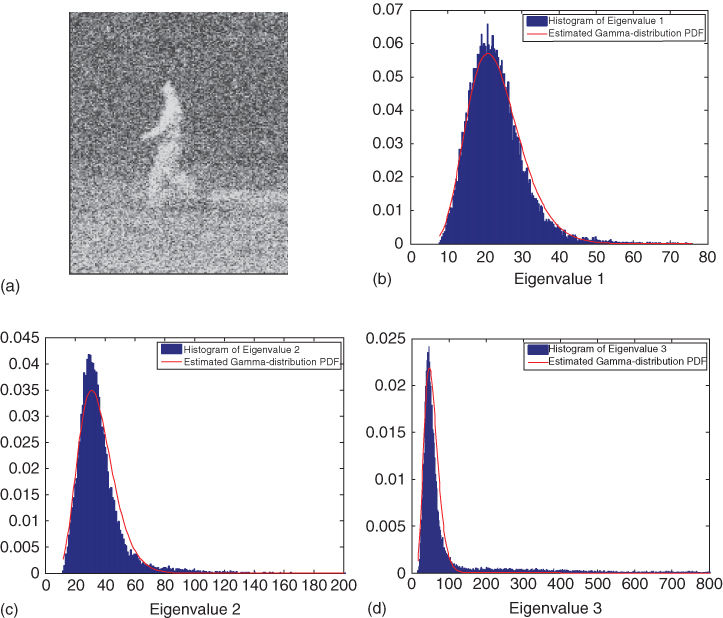
Figure 16.6 (a) One frame of an amplified noisy image sequence. (b)–(d) Histograms of eigenvalues 1–3 in blue. Also shown in red are fitted gamma distributions to the data.

From the gamma distribution means, , and variances, , can be estimated. These parameters can be used to set the parameters, that is, , of the algorithm.

16.5.2 Parallelization and Computational Aspects

The visual system of most animals is based on a highly parallel architecture. On looking at the overview of Algorithm 16.1, two things are clear. The algorithm is linear in the number of voxels in the input image sequence and it is highly parallelizable. The output of each voxel depends only on a neighborhood of that given voxel. The most expensive parts are the calculation of the structure tensor, including the gradient calculation, the elementwise smoothing, and the actual filtering, or summation. This is a task for which the graphics processing units of modern graphics cards are very well suited.

We have implemented the whole adaptive enhancement methodology as a combined CPU/GPU algorithm. All image pre- and postprocessing is performed on the CPU. This includes image input/output and the amplification step. If we use histogram equalization as a contrast amplification, this requires summation over all pixels. This computation is not easily adapted to a GPU, as the summation would have to be done in multiple passes. However, as these steps constitute a small part of the execution time, a simpler CPU implementation is adequate here. In summary, by exploiting the massively parallel architecture of modern GPUs, we obtain interactive frame rates on a single nVidia GeForce 8800-series graphics card.

16.5.3 Considerations for Color

The discussion so far has dealt with intensity images. We now discuss some special aspects of the algorithm when it comes to processing color images.

In applying the algorithm to RGB color image data, one could envision a procedure where the color data in the images are first transformed to another color space including an intensity channel, for example, the HSV color space, cf. Ref. [71]. The algorithm could then be applied unaltered to the intensity channel, while smoothing of the other two channels could either be performed with the same kernel as in the intensity channel or by isotropic smoothing. The HSV image would then be transformed back to the RGB color space.

However, in very dark color video sequences there is often a significant difference in the noise levels in the different input channels: for example, the blue channel often has a relatively higher noise level. It is therefore essential that it is possible to adapt the algorithm to this difference. To this end, we chose to calculate the structure tensor , and its eigenvectors and eigenvalues, in the intensity channel, which we simply define as the mean of the three color channels. The widths of the kernels are then adjusted separately for each color channel by using a different value of the scaling parameter for each channel. This gives a clear improvement of the output with colors that are closer to the true chromaticity values and with less false color fluctuations than in the above-mentioned HSV approach.

When acquiring raw image data from a CCD or CMOS sensor, the pixels are usually arranged according to the so-called Bayer pattern. It has been shown, cf. Ref. [90], that it is efficient and suitable to perform the interpolation from the Bayer pattern to three separate channels, so-called demosaicing, simultaneously to the denoising of the image data. We apply this approach here for each channel, by setting to zero the coefficients in the summation kernel corresponding to pixels where the intensity data is not available and then normalizing the kernel. A smoothed output is then calculated for both the noisy input pixels and the pixels where data are missing.

16.5.4 Experimental Results

In this section, we describe some experimental results. We have tested our algorithm on a number of different types of sequences involving static and moving scenes and with large or little motion of the camera. We have also used a number of different cameras, ranging from cheap consumer cameras to high-end machine vision cameras. We have compared our method to a number of different methods described in the related work section, but most algorithms are not targeted at low-light vision and cannot handle the resulting levels of noise. The algorithm that gives comparable results to ours is BM3D for video, Ref. [21]. We have used the implementation from Ref. [91].

In Figure 16.7, the results of running our algorithm are shown for a number of different input sequences. Also shown is the result of running BM3D. In Figure 16.8, a close-up is shown for two of the frames from Figure 16.7. One can see that BM3D gives very sharp results with very little noise left. In this sense the quality is slightly better than our approach. However, owing to the high noise levels, two types of artifacts can be noticed in the BM3D images: the block structure is visible and we get hallucination effects due to the codebook nature of BM3D. This results in small objects appearing or disappearing.

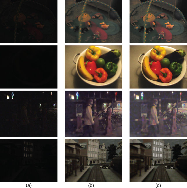
Figure 16.7 Illustration of results from four different input sequences. (a) One frame of the dark input sequence. (b) One frame of our approach and (c) one frame of the result of running BM3D. The two top rows were taken by a standard compact digital camera, a Canon IXUS 800 IS. The third row was taken by a handheld consumer camcorder, a Sony DCR-HC23. The bottom row was taken by an AVT Marlin machine vision camera. The two top and the bottom sequences have large camera motions and the two bottom sequences have additional motion in the scene.

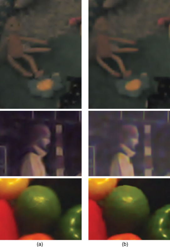
Figure 16.8 A close-up of one frame from the output sequences. (a) The result using our approach and (b) the result using BM3D. One can see that BM3D gives very sharp edges but in some cases, it hallucinates and removes parts due to the codebook nature of BM3D. One can also see some blocking artifacts due to the block structure of BM3D.

In order to test the noise reduction part of our method, we conducted a semisynthetic experiment in the following way. We recorded a video sequence under good lighting conditions. This resulted in a sequence with very little noise. We then synthetically constructed a low-light video sequence by dividing the 8-bit gray values by a constant (e.g., 50), added Gaussian noise with standard deviation (e.g., 1), and finally truncated the gray values to integer values. We then amplified the sequence by multiplying by . This gave us a highly noisy sequence, with known ground truth. One frame of the dark sequence can be seen in second row Figure 16.7. We ran our noise reduction step and compared it to BM3D. The resulting peak signal-to-noise ratio (PSNR) and the structure similarity (SSIM) index [92] can be seen in Table 16.1together with the values for the initial noisy amplified signal. The results for our method and BM3D are very similar. The difference is that our method gives less sharp results, while BM3D gives more blocking artifacts. In terms of computational complexity, the two methods are comparable. As described in Section 16.5.2, our smoothing method is linear in the number of processed voxels, but the factor is highly dependent on the size of the summation neighborhood. This is also true for BM3D which is highly dependent on the size of the block matching neighborhood.

Table 16.1 Peak signal to noise-ratio (PSNR) and structural similarity (SSIM) index for the semisynthetic test sequence

16.6 Conclusions

The colors and contrasts of the nocturnal world are just as rich as those found in the diurnal world, and many animals – both vertebrate and invertebrate – have evolved visual systems to exploit this abundant information. Via a combination of highly sensitive optical eye designs and unique alterations in the morphology, circuitry, and physiology of the retina and higher visual centers, nocturnal animals are capable of advanced and reliable vision at night. In the case of the nocturnal bee Megalopta genalis, greatly enlarged corneal facets and rhabdoms and slow photoreceptors with high contrast gain ensure that visual signal strength is maximal as it leaves the eye and travels to the lamina. Even though it remains to be shown conclusively, anatomical and theoretical evidence suggests that once the visual signals from large groups of ommatidia reach the lamina, they are spatially (and possibly temporally) summed by the second-order monopolar cells, resulting in an enhanced signal and reduced noise. The greatly improved SNR that this strategy could afford, while confined to a narrower range of spatial and temporal frequencies, would ensure that nocturnal visual reliability is maximized for the slower and coarser features of the world. Those features that are faster and finer – and inherently noisy – would be filtered out. But slower and coarser features, in contrast, would be seen more clearly. Using these biological principles as inspiration, we have developed a night-vision algorithm that processes and enhances video sequences captured in very dim light. This algorithm, similarly to a nocturnal visual system, relies on initial amplification of image signals and a local noise-reducing spatiotemporal summation that is weighted by the extent of image motion occurring in the same image locality. The algorithm dramatically increases the visibility of image features, including the preservation of edges, forms, and colors. This could be used in a number of applications, that is, improving videos taken at night or in dim rooms. It could also be used for surveillance purposes. One of our goal application areas has been in improving vehicular video data, which in turn could be used for example, for pedestrian detection, obstacle avoidance, or traffic sign detection.

Our method provides not only a significant result in the field of dim-light image processing but it also strengthens the evidence that summation strategies are essential for reliable vision in nocturnal animals.

Acknowledgment

The authors are indebted to Toyota Motor Engineering & Development Europe, the US Air Force Office of Scientific Research (AFOSR), and the Swedish ResearchCouncil for their financial support.

References

1. 1. Warrant, E.J. and Dacke, M. (2011) Vision and visual navigation in nocturnal insects. Annu. Rev. Entomol., 56, 239–254.

2. 2. Kelber, A., Balkenius, A., and Warrant, E.J. (2002) Scotopic colour vision in nocturnal hawkmoths. Nature, 419, 922–925.

3. 3. Somanathan, H., Borges, R.M., Warrant, E.J., and Kelber, A. (2008) Nocturnal bees learn landmark colours in starlight. Curr. Biol., 18 (21), R996–R997.

4. 4. Theobald, J., Warrant, E.J., and O'Carroll, D.C. (2010) Wide-field motion tuning in nocturnal hawkmoths. Proc. R. Soc. London, Ser. B, 277, 853–860.

5. 5. Baird, M., Kreiss, E., Wcislo, W.T., Warrant, E.J., and Dacke, M. (2011) Nocturnal insects use optic flow for flight control. Biol. Lett., 7, 499–501.

6. 6. Warrant, E.J. (2004) Vision in the dimmest habitats on earth. J. Comp. Physiol. A, 190, 765–789.

7. 7. Somanathan, H., Borges, R.M., Warrant, E.J., and Kelber, A. (2008) Visual ecology of Indian carpenter bees I: light intensities and flight activity. J. Comp. Physiol. A, 194, 97–107.

8. 8. Reid, S.F., Narendra, A., Hemmi, J.M., and Zeil, J. (2011) Polarised skylight and the landmark panorama provide night-active bull ants with compass information during route following. J. Exp. Biol., 214, 363–370.

9. 9. Dacke, M., Nilsson, D.E., Scholtz, C.H., Byrne, M., and Warrant, E.J. (2003) Insect orientation to polarized moonlight. Nature, 424, 33.

10.10. Dacke, M., Baird, E., Byrne, M., Scholtz, C.H., and Warrant, E.J. (2013) Dung beetles use the Milky Way for orientation. Curr. Biol., 23, 298–300.

11.11. Malm, H. and Warrant, E. (2006) Motion dependent spatiotemporal smoothing for noise reduction in very dim light image sequences. Proceedings International Conference on Pattern Recognition, Hong Kong, pp. 954–959.

12.12. Malm, H., Oskarsson, M., Warrant, E., Clarberg, P., Hasselgren, J., and Lejdfors, C. (2007) Adaptive enhancement and noise reduction in very low light-level video. IEEE 11th International Conference on Computer Vision, 2007. ICCV 2007, IEEE, pp. 1–8.

13.13. Malm, H., Oskarsson, M., and Warrant, E. (2012) Biologically inspired enhancement of dim light video, Frontiers in Sensing, Springer-Verlag, pp. 71–85.

14.14. Warrant, E., Oskarsson, M., and Malm, H. (2014) The remarkable visual abilities of nocturnal insects: neural principles and bioinspired night-vision algorithms. Proc. IEEE, 102 (10), 1411–1426.

15.15. Kalivas, D. and Sawchuk, A. (1990) Motion compensated enhancement of noisy image sequences. Proceedings IEEE International Conference Acoustics Speech, and Signal Processing, Alburquerque, NM, pp. 2121–2124.

16.16. Özkan, M., Sezan, M., and Tekalp, A. (1993) Adaptive motion-compensated filtering of noisy image sequences. IEEE Tran. Circuits Syst. Video Technol., 3 (4), 277–290.

17.17. Miyata, K. and Taguchi, A. (2002) Spatio-temporal separable data-dependent weighted average filtering for restoration of the image sequences. Proceedings IEEE International Conference on Acoustics, Speech and Signal Processing, vol. 4, Alburquerque, NM, pp. 3696–3699.

18.18. Sezan, M., Özkan, M., and Fogel, S. (1991) Temporally adaptive filtering of noisy image sequences. Proceedings IEEE International Conference on Acoustics, Speech and Signal Processing, vol. 4, Toronto, Canada, pp. 2429–2432.

19.19. Dugad, R. and Ahuja, N. (1999) Video denoising by combining kalman and wiener estimates. Proceedings International Conference on Image Processing, vol. 4, Kobe, Japan, p. 152–156.

20.20. Buades, A., Coll, B., and Morel, J.M. (2005) A non-local algorithm for image denoising. IEEE Computer Society Conference on Computer Vision and Pattern Recognition, 2005. CVPR 2005, vol. 2, IEEE, pp. 60–65.

21.21. Dabov, K., Foi, A., and Egiazarian, K. (2007) Video denoising by sparse 3d transform-domain collaborative filtering. Proceedings of the 15th European Signal Processing Conference, vol. 1, p. 7.

22.22. Dabov, K., Foi, A., Katkovnik, V., and Egiazarian, K. (2007) Image denoising by sparse 3-d transform-domain collaborative filtering. IEEE Trans. Image Process., 16 (8), 2080–2095.

23.23. Martinez, D. and Lim, J. (1985) Implicit motion compensated noise reduction of motion video signals. Proceedings IEEE International Conference on Acoustics, Speech and Signal Processing, Tampa, FL, pp. 375–378.

24.24. Arce, G. (1991) Multistage order statistic filters for image sequence processing. IEEE Trans. Signal Proc., 39 (5), 1146–1163.

25.25. Ko, S.J., and Forest, T. (1993) Image sequence enhancement based on adaptive symmetric order statistics. IEEE Trans. Circuits Syst. II: Analog Digital Signal Proc., 40 (8), 504–509.

26.26. Brailean, J., Kleihorst, R., Efstratiadis, S., Katsaggelos, A., and Lagendijk, R. (1995) Noise reduction filters for dynamic image sequences: a review. Proc. IEEE, 83 (9), 1272–1289.

27.27. Perona, P. and Malik, J. (1990) Scale-space and edge detection using anisotropic diffusion. IEEE Trans. Pattern Anal. Mach. Intell., 12 (7), 629–639.

28.28. Weickert, J. (1998) Anisotropic Diffusion in Image Processing, Teubner-Verlag, Stuttgart.

29.29. Uttenweiler, D., Weber, C., Jähne, B., Fink, R., and Scharr, H. (2003) Spatiotemporal anisotropic diffusion filtering to improve signal-to-noise ratios and object restoration in fluorescence microscopic image sequences. J. Biomed. Opt., 8 (1), 40–47.

30.30. Lee, S. and Kang, M. (1998) Spatio-temporal video filtering algorithm based on 3-d anisotropic diffusion equation. Proceedings International Conference on Image Processing, vol. 2, pp. 447–450.

31.31. Weickert, J. (1999) Coherence-enhancing diffusion filtering. Int. J. Comput. Vision, 31 (2-3), 111–127.

32.32. Tomasi, C. and Manduchi, R. (1998) Bilateral filtering for gray and color images. Proceedings of the 6th International Conference Computer Vision, pp. 839–846.

33.33. Yang, G., Burger, P., Firmin, D., and Underwood, S. (1996) Structure adaptive anisotropic image filtering. Image Vision Comput., 14, 135–145.

34.34. Barash, D., and Comaniciu, D. (2004) A common framework for nonlinear diffusion, adaptive smoothing, bilateral filtering and mean shift. Image Vision Comput., 22, 73–81.

35.35. Kang, S., Uytendaele, M., Winder, S., and Szeliski, R. (2003) High dynamic range video. SIGGRAPH '03: ACM SIGGRAPH 2003 Papers, pp. 319–325.

36.36. Reinhard, E., Ward, G., Pattanaik, S., and Debevec, P. (2005) High Dynamic Range Imaging: Acquisition, Display, and Image-Based Lighting, Morgan Kaufmann Publishers.

37.37. Bennett, E. and McMillan, L. (2005) Video enhancement using per-pixel virtual exposures. Proceedings SIGGRAPH, Los Angeles, CA, pp. 845–852.

38.38. Lee, S.W., Maik, V., Jang, J., Shin, J., and Paik, J. (2005) Noise-adaptive spatio-temporal filter for real-time noise removal in low light level images. IEEE Tran. Consum. Electron., 51 (2), 648–653.

39.39. Martin, G.R. (1990) Birds By Night, T. and A.D. Poyser, London.

40.40. Warrant, E.J. (2008) Nocturnal vision, in The Senses: A Comprehensive Reference (Vol. 2: Vision II) (eds T. Albright and R. Masland), Academic Press, pp. 53–86.

41.41. Laughlin, S.B. (1990) Invertebrate vision at low luminances, in Night Vision (eds R.F. Hess, L.T. Sharpe, and K. Nordby), Cambridge University Press, pp. 223–250.

42.42. Warrant, E.J. (2006) The Sensitivity of Invertebrate Eyes to Light (E.J. Warrant and D.-E. Nilsson Invertebrate Vision), Cambridge University Press, Cambridge, pp. 167–210.

43.43. Lillywhite, P.G. and Laughlin, S.B. (1979) Transducer noise in a photoreceptor. Nature, 277, 569–572.

44.44. Frederiksen, R., Wcislo, W.T., and Warrant, E.J. (2008) Visual reliability and information rate in the retina of a nocturnal bee. Curr. Biol., 18, 349–353.

45.45. Rose, A. (1942) The relative sensitivities of television pickup tubes, photographic film and the human eye. Proc. Inst. Radio Eng. N. Y., 30, 293–300.

46.46. de Vries, H.L. (1943) The quantum character of light and its bearing upon threshold of vision, the differential sensitivity and visual acuity of the eye. Physica, 10, 553–564.

47.47. Land, M.F. (1981) Optics and vision in invertebrates, in Handbook of Sensory Physiology, V. VII/6B (ed. H. Autrum), Springer-Verlag, Berlin, Heidelberg and New York, pp. 471–592.

48.48. Lillywhite, P.G. (1977) Single photon signals and transduction in an insect eye. J. Comp. Physiol., 122, 189–200.

49.49. Laughlin, S.B. and Lillywhite, P.G. (1982) Intrinsic noise in locust photoreceptors. J. Physiol., 332, 25–45.

50.50. Barlow, H.B. (1956) Retinal noise and absolute threshold. J. Opt. Soc. Amer., 46, 634–639.

51.51. Dubs, A., Laughlin, S.B., and Srinivasan, M.V. (1981) Single photon signals in fly photoreceptors and first order interneurons at behavioural threshold. J. Physiol., 317, 317–334.

52.52. Doujak, F.E. (1985) Can a shore crab see a star? J. Exp. Biol., 166, 385–393.

53.53. Baylor, D.A., Matthews, G., and Yau, K.W. (1980) Two components of electrical dark noise in toad retinal rod outer segments. J. Physiol., 309, 591–621.

54.54. Aho, A.C., Donner, K., Hydén, C., Larsen, L.O., and Reuter, T. (1988) Low retinal noise in animals with low body temperature allows high visual sensitivity. Nature, 334, 348–350.

55.55. Aho, A.C., Donner, K., Helenius, S., Larsen, L.O., and Reuter, T. (1993) Visual performance of the toad (Bufo bufo) at low light levels, retinal ganglion cell responses and prey-catching accuracy. J. Comp. Physiol. A, 172, 671–682.

56.56. Healey, G.E. and Kondepudy, R. (1994) Radiometric CCD camera calibration and noise estimation. IEEE Trans. Pattern Anal. Mach. Intell., 16 (3), 267–276.

57.57. Laughlin, S.B. and Weckström, M. (1993) Fast and slow photoreceptors: a comparative study of the functional diversity of coding and conductances in the Diptera. J. Comp. Physiol. A, 172, 593–609.

58.58. Laughlin, S.B., Blest, A.D., and Stowe, S. (1980) The sensitivity of receptors in the posterior median eye of the nocturnal spider Dinopis. J. Comp. Physiol., 141, 53–65.

59.59. Heimonen, K., Salmela, I., Kontiokari, P., and Weckström, M. (2006) Large functional variability in cockroach photoreceptors: optimization to low light levels. J. Neurosci., 26, 13454–13462.

60.60. Pirhofer-Walzl, K., Warrant, E.J., and Barth, F.G. (2007) Adaptations for vision in dim light: impulse responses and bumps in nocturnal spider photoreceptor cells (Cupiennius salei Keys). J. Comp. Physiol. A, 193, 1081–1087.

61.61. Horridge, G., Duniec, J., and Marčelja, L. (1981) A 24-hour cycle in single locust and mantis photoreceptors. J. Exp. Biol., 91 (1), 307–322.

62.62. Greiner, B., Ribi, W.A., Wcislo, W.T., and Warrant, E.J. (2004) Neuronal organisation in the first optic ganglion of the nocturnal bee Megalopta genalis. Cell Tissue Res., 318, 429–437.

63.63. Ribi, W. (1975) The first optic ganglion of the bee. Cell Tissue Res., 165 (1), 103–111.

64.64. Hateren, J.Hv. (1992) Real and optimal neural images in early vision. Nature, 360, 68–70.

65.65. Hateren, J.Hv. (1993) Spatiotemporal contrast sensitivity of early vision. Vision Res., 33, 257–267.

66.66. Laughlin, S.B. (1996) Matched filtering by a photoreceptor membrane. Vision Res., 36, 1529–1541.

67.67. Weckström, M. and Laughlin, S.B. (1995) Visual ecology and voltage-gated ion channels in insect photoreceptors. Trends Neurosci., 18 (1), 17–21.

68.68. Niven, J.E., Vähäsöyrinki, M., Kauranen, M., Hardie, R.C., Juusola, M., and Weckström, M. (2003) The contribution of shaker K+ channels to the information capacity of Drosophila photoreceptors. Nature, 421 (6923), 630–634.

69.69. Niven, J.E., Anderson, J.C., and Laughlin, S.B. (2007) Fly photoreceptors demonstrate energy-information trade-offs in neural coding. PLoS Biol., 5 (4), e116.

70.70. Drago, F., Myszkowski, K., Annen, T., and Chiba, N. (2003) Adaptive logarithmic mapping for displaying high contrast scenes. Proceedings EUROGRAPHICS, vol. 22, pp. 419–426.

71.71. Gonzalez, R. and Woods, R. (1992) Digital Image Processing, Addison-Wesley.

72.72. Pizer, S., Amburn, E., Austin, J., Cromartie, R., Geselowitz, A., Geer, T., teer Haar Romeny, B., Zimmerman, J., and Zuiderveld, K. (1987) Adaptive histogram equalization and its variations. Comput. Vision Graph. Image Process., 39, 355–368.

73.73. Snyder, A.W. (1977) Acuity of compound eyes, physical limitations and design. J. Comp. Physiol., 116, 161–182.

74.74. Snyder, A.W., Laughlin, S.B., and Stavenga, D.G. (1977) Information capacity of eyes. Vision Res., 17, 1163–1175.

75.75. Snyder, A.W., Stavenga, D.G., and Laughlin, S.B. (1977) Spatial information capacity of compound eyes. J. Comp. Physiol., 116, 183–207.

76.76. Laughlin, S.B. (1981) Neural principles in the peripheral visual systems of invertebrates, in Handbook of Sensory Physiology, V. VII/6B (ed. H. Autrum), Springer-Verlag, Berlin, Heidelberg and New York, pp. 133–280.

77.77. Warrant, E.J. (1999) Seeing better at night: life style, eye design and the optimum strategy of spatial and temporal summation. Vision Res., 39, 1611–1630.

78.78. Greiner, B., Ribi, W.A., and Warrant, E.J. (2005) A neural network to improve dim-light vision? Dendritic fields of first-order interneurons in the nocturnal bee Megalopta genalis. Cell Tissue Res., 323, 313–320.

79.79. Ribi, W.A. (1977) Fine structure of the first optic ganglion (lamina) of the cockroach, Periplaneta Americana. Tissue Cell, 9, 57–72.

80.80. Ohly, K.P. (1975) The neurons of the first synaptic regions of the optic neuropil of the firefly Phausius splendidula L. (Coleoptera). Cell Tissue Res., 158, 89–109.

81.81. Strausfeld, N.J. and Blest, A.D. (1970) Golgi studies on insects I. The optic lobes of Lepidoptera. Philos. Trans. R. Soc. London, Ser. B, 258, 81–134.

82.82. Theobald, J.C., Greiner, B., Wcislo, W.T., and Warrant, E.J. (2006) Visual summation in night-flying sweat bees: a theoretical study. Vision Res., 46, 2298–2309.

83.83. Klaus, A. and Warrant, E.J. (2009) Optimum spatiotemporal receptive fields for vision in dim light. J. Vision, 9 (4), 1–16.

84.84. Warrant, E.J., Porombka, T., and Kirchner, W.H. (1996) Neural image enhancement allows honeybees to see at night. Proc. R. Soc. London, Ser. B, 263, 1521–1526.

85.85. Jähne, B. (1993) Spatio-Temporal Image Processing, Springer-Verlag.

86.86. Bigun, J. and Granlund, G.H. (1987) Optimal orientation detection of linear symmetry. Proceedings of the IEEE 1st International Conference on Computer Vision, London, Great Britain, pp. 433–438.

87.87. Knutsson, H. (1989) Representing local structure using tensors. The 6th Scandinavian Conference on Image Analysis, Oulu, Finland, pp. 244–251.

88.88. Haussecker, H. and Spies, H. (1999) Handbook of Computer Vision and Applications, vol. 2, Chap. Motion, Academic Press, pp. 125–151.

89.89. Atick, J.J. (1992) Could information theory provide an ecological theory of sensory processing? Netw. Comput. Neural Syst., 3 (2), 213–251.

90.90. Hirakawa, K. and Parks, T. (2006) Joint demosaicing and denoising. IEEE Trans. Image Process., 15 (8), 2146–2157.

91.91. http://www.cs.tut.fi/foi/GCF-BM3D/.

92.92. Wang, Z., Bovik, A.C., Sheikh, H.R., and Simoncelli, E.P. (2004) Image quality assessment: from error visibility to structural similarity. IEEE Trans. Image Process., 13 (4), 600–612.