Biologically Inspired Computer Vision (2015)

Part IV
Applications

Chapter 17
Bioinspired Motion Detection Based on an FPGA Platform

Tim Köhler

17.1 Introduction

Visual detection of motion is one of the computer vision methods that has been in high demand. Several applications of motion detection can be found in mobile robotics, for example, obstacle avoidance or flight stabilization of unmanned air vehicles. In the case of small and light robots, particularly, computer vision processing has been very limited because of power consumption and weight. As flying insects are able to solve the same tasks with very limited processing and power resources, biologically inspired methods promise to provide very efficient solutions. However, even if a biological solution for a computer vision task is found, in an application, the manner in which this solution is implemented is also of critical importance.

In this chapter, the combination of (a) a bioinspired motion detection method and (b) a very versatile design flow is presented. The implementation described here uses specific devices called field-programmable gate arrays (FPGAs). Such a hardware design process allows an implementation which is very well adapted to an algorithm and, thus, can lead to a very efficient implementation.

This chapter's scope covers topics discussed at greater length in other chapters. For more details on compound- and biosensors, see Chapters 6 and 12 which focuses on the topic of motion detection.

Section 17.2 provides a short motivation for hardware implementation of biologically inspired computer vision in motion detection. Section 17.3 gives an introduction to insect motion detection. The results of behavioral biology and neural biology studies are summarized therein. Section 17.4 presents an overview of findings on robotic implementations of biological insectmotion detection. This includes solutions using FPGA and, therefore, a short introduction to FPGAs as well. The main part of this chapter is Section 17.5. in which an FPGA-based module implementing bioinspired motion detection is described. Section 17.6shows experimental results of the motion detection module. Finally, Section 17.7 discusses the implementation and the experimental results and Section 17.8 concludes the chapter.

17.2 A Motion Detection Module for Robotics and Biology

Visual detection of motion is realized in biology in a very efficient and reliable manner. Insects such as flies are capable of detecting an approaching object very quickly. On the other hand, the incorporated resources for this motion detection are quite limited. For example, the housefly Musca domestica has compound eyes with only about 3000 single facets (called ommatidia). Furthermore, the neural processing for the detection of motion is also limited (see Section 17.3). Taking all these factors into account, the fly has the ability for quick visual detection of motion with little processing, its low weight, small size, and a very small energy consumption.

This efficient biological motion detection¹ gives a very interesting blueprint for technical motion detection applications. So-called micro air vehicles (MAV), for example, face problems comparable to those of flying insects (flight stabilization, obstacle detection). They cannot use powerful computers to solve these tasks because of size and weight limitations. Having an efficient implementation derived from biology could solve such problems. Therefore, implementing the biological findings in engineering in an efficient manner is needed. There are many examples of such implementations that have been published (see Refs [1, 2], and [3]).

A second motivation can be found in biorobotics in general: the flow of scientific findings is not always in the direction from biology to robotics. Instead, the opposite direction can also be of importance . In biology, explanatory models can be set up on the basis of behavioral experiments. Insect motion detection, as an example, was studied in the 1950s by Hassenstein and Reichardt [4]. Such behavioral studies can lead to models that explain the observed behaviors. But to be certain that a stated model is a correct explanation, the opposite direction need to be tested; that is, using a synthetic implementation of the proposed model to perform the tasks studied in the behavioral experiments. Such a synthetic implementation could be realized and tested in computer simulations. However, to arrive at acceptable results, the test conditions often need to be as realistic as possible (real environment,comparable optical parameters such as spatial and temporal resolution). This is why a robotic implementation of a model is necessary. Of course, a verification via such a synthetic model alone is still not be proof regarding the correctness of the proposed model. But if the synthetic implementation fails to show the behavior noticed in the behavioral experiments – that is, even under optimal conditions, it is very likely that the proposed model would fail in the real biological counterpart, too, and therefore it is not valid. The option of carrying out neural measurements in living insects is chosen in neural biology. However, even with this method, finding all three parts, namely, preprocessing, motion detection, and postprocessing, may not be feasible. Thus, there is sufficient motivation for a computer vision implementation both in robotics and in biology.

17.3 Insect Motion Detection Models

The insect visual system can be separated into two parts: first, there is the so-called compound eye with optical and receptive neural components and, second, there is the further neural processing. A sketch of a compound eye can be seen in Figure 17.1(a) and a single photoreception unit (called ommatidium) in Figure 17.1(b). This structure is an example; different variations of this can also be found. One variation is optical superposition (no complete separation of the ommatidia by pigment cells); another is the number of photoreceptor cells per ommatidium. Some more details can be found in Ref. [5].

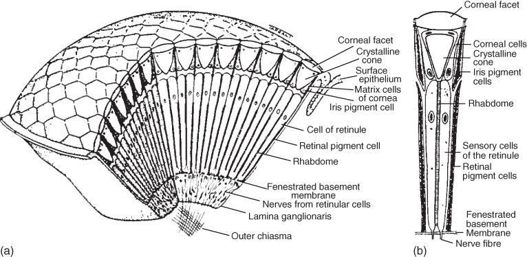
Figure 17.1 (a) The section of a compound eye. Exemplarily, the ommatidia are optically separated here. This is not the case for all complex eyes. (b) The section of an ommatidium (again with an optical separation from the neighbor ommatidia). (Adapted from Ref. [[6], pages 155 and 167]).

A diagram of both parts (compound eye and further neural processing) is depicted in Figure 17.2. Most of the motion detection components of insect vision are located or supposed to be located in the further neural processing, that is,. in the lamina, the lobula plate, and the medulla [7, 8].

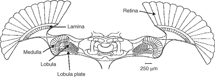
Figure 17.2 Schematic horizontal cross section through the head of a fly including the major parts of its head ganglion (adapted from Ref. [7], Figure 1, with kind permission from Springer Science and Business Media).

Insect motion detection has been studied from the 1950s. One of the first findings was the identification of a separation in local detection components, on the one hand, and an integration of multiple local detection signals, on the other. Through integration, a detection signal for a larger region covering the whole field of view is generated. The single local detection components are referred to as elementary motion detectors (EMD) in the following.

Figure 17.3 illustrates three different versions of EMD . A feature common to all three is that the signals of only two photoreceptors (or two groups of photoreceptors) are used to detect motion components along one (called preferred) motion vector from one of the receptors (or the receptor groups) to the other [9]. For motion (components) in the direction from the first to the second receptor (in the figures, from the left to the right receptor) the detector generates a positive output value. For motion in the opposite direction, the output is negative.

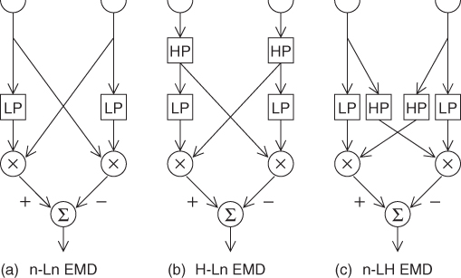
Figure 17.3 (a), (b), and (c) Three versions of EMDs. The “” on top denotes a photoreceptor. “LP” and “HP” stand for lowpass filter and highpass filter, respectively. The correlation component “” can be realized by a multiplication and “” by a summation (see text). The labels below the figures are used to refer to these models. The labels conform to a naming scheme in which the first letter represents the input stage (in this case, with a highpass input filter “H” or with no preprocessing “n”). The following two letters stand for the components between the preprocessing and the correlation inputs: The first letter identifies the component before the first correlation input (vertical arms in the figures, in these three models, all are lowpass filters “L”). The second letter represents the component in front of the second correlation inputs (the crossed arms in the figures, highpass filters “H” or no filter operations “n”). Such symmetrical models are sometimes referred to as “full-detector,” while one half of these detectors (i.e., just one correlation element and no summation) are sometimes called “half-detector” (figures taken from Refs. [10, 11]). © IOP Publishing. Reproduced by permission of IOP Publishing. All rights reserved.

The simplest EMD version can be seen in Figure 17.3(a). Here, the signals of the two photoreceptors are delayed by a lowpass filter component. The delayed signal of one receptor (i.e., the output of one of the lowpass filters) is correlated with the undelayed signal of the other receptor (see the review of Egelhaaf and Borst [12]). As correlation function, a simple multiplication leads to results that are comparable to biological data. Finally, the difference between the two correlation results needs to be computed.

The resulting behavior is as follows (see Figure 17.4): if an object moves from a position in front of the left photoreceptor to a position in front of the right receptor then the corresponding reflected brightness values will be perceived first by the left receptor and after a certain delay (depending on the object's motion speed), by the right receptor. If the motion speed matches the delay in the left receptor's lowpass filter, then the corresponding brightness values are correlated at one of the multiplication components. This correspondence leads to high correlation results, while the second multiplication component is supplied with uncorrelated brightness values (leading to small correlation values). As a result, the small correlation value is subtracted from the large correlation value and the detector's output value is large.

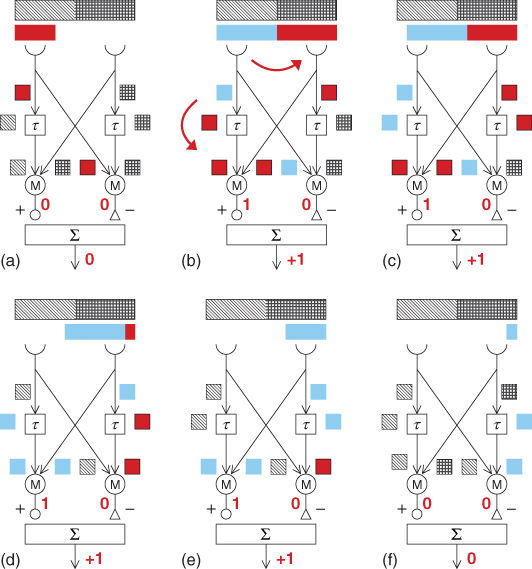
Figure 17.4 Functionality of the EMD. Exemplarily, a red and blue object moves from the left-hand side to the right-hand side. Depicted are six states (a)–(f). The “” denotes a delay element (see text) and “M” a correlation.

In case of motion in the opposite direction, a large value is subtracted from a small value leading to a large negative output. Finally, in case of no motion (in the direction between the two receptors), both correlation results are equal and the detector's output will be zero. The two computation parts up to one correlation (left-hand side, right-hand side) are sometimes called “half-detectors” and could be used alone if only one motion direction is to be detected. If the delay induced by the motion velocity and the lowpass filters' delays do not match, then the correlation result will be less than optimal and the absolute value of the detector's output will be less than the maximum output. At very slow or very fast motion speed, the detector's output might not be distinguishable from zero.

As Harris et al. [13] have shown, the simple EMD's response differs from empirical data. This is especially the case for specific pattern types and motion conditions (see Ref. [14]). A proposed improvement is the introduction of a first-order highpass filter to suppress constant illumination differences as depicted in Figure 17.3(b) (see Ref. [15]).

A further variation was proposed by Kirschfeld [16] (see also [15]) and can be seen in Figure 17.3(c). Two of the advantages of this version are, first, again a better correspondence to biological data under specific conditions and, second, a stronger response compared to a H-Ln EMD (see caption of Figure 17.3) with the same time constants.

There are further variants of EMD types, some of which have been published quite recently. For example, Ref. [17] presents two versions with a reduced sensitivity to contrast changes. This property is especially interesting for motion detection in mobile robots.

A feature common for all these variations is that a single EMD uses just two photoreceptors (or two local photoreceptor groups). However, to generate a reliable detector response the output values of multiple EMDs are combined. A simple realization is a summation of the single EMD responses – which is sufficient in terms of an acceptable accordance with biological data and sufficient for many robotic applications. Two effects of such an aggregation are an increased reliability and a better ratio of motion-induced detector response to nonsystematic responses (signal-to-noise ratio, SNR). However, probably the main advantage of a combination of several (locally detecting) EMDs is the detectability of (a) regional/global motion and (b) complex motion types. In Figure 17.5 three examples are depicted.

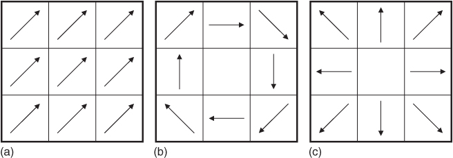
Figure 17.5 By the aggregation of several EMD responses to EMD arrays (covering up to the whole field of view), specific types of motion can be detected. For the sake of simplicity, all examples show a quadratic field of view of up to nine EMDs. The arrows depict single EMDs with the respective preferred direction. (a) The EMD array responds strongest to its preferred motion direction from the bottom left to the top right. (b) The array has a clockwise rotation as preferred optical flow . (c) The EMD array responds strongest to approaching objects, leading to “looming” optical flow (figures taken from Refs [10, 11]).

As an alternative to a simple summation of the single EMD responses [18] suggest a nonlinear passive membrane model. Extensions or modifications such as this—also of the EMDs' filters or correlation—have been proposed several times after the original publications by Hassenstein and Reichardt. Often they lead to detector responses which fit better to measurements of the biological counterpart. Another example of this is a weighting of the single EMD responses (leading to so-called “matched filters”) which was proposed by Franz and Krapp [19].

Expected steady-state responses to a constantly moving sine pattern for the H-Ln- and the n-LH-EMD type (see caption of Figure 17.3) were derived by Borst et al. [15]. The estimations are based on the ideal behavior of first-order, lowpass and first-order, highpass filters. The expected steady-state response of a H-Ln-EMD to a constantly moving sine pattern is derived by Borst et al. [15] as shown in Eq. (17.1). Given is the average value of multiple detectors, each with a different position, that is, a different phase . The stimulus is generated by a sine pattern with period length moved with constant velocity . The resulting stimuli at the receptors have a frequency of . The time constants and are those of the lowpass filters and the highpass filters, respectively. Note that , the constant DC component of the stimulus (depending on the constant average of the illumination and the constant average of the pattern brightness), is not included in the given equation. Thus, the detector's output signal does not depend on these constant properties. Of course, the amplitude of the input signal () has a major influence on the detector's response.

17.1

In Eq. (17.2), the expected steady-state response of the n-LH type detector array when excited with the same constantly moving sine pattern can be seen. Both theoretical steady-state responses are compared with measurements in the experiments Section 17.6 below.

17.2

These two equations are needed in the experimental Section 17.6. Further explanations and theoretical ideal responses are given by Borst et al. [15].

17.4 Overview of Robotic Implementations of Bioinspired Motion Detection

For the implementation of bioinspired algorithms in general, the methods and types of hardware used could be like those for any other application. However, as often one motivation to use a biologically inspired algorithm is power/weight efficiency, the hardware basis for such an implementation needs to be selected accordingly.

There are generally two options for algorithmic implementations:

1. Implementation in software

2. Implementation in hardware.

In case of the EMD-based motion detection, there are some publications presenting implementations of option (1). Zanker and Zeil [20] propose a software implementation which runs on a standard personal computer. With respect to the power and/or weight limitations of several EMD-applications (especially micro air vehicles, but also typical mobile robots), the need for a PC is often a knockout criterion. An alternative software implementation was presented by Ruffier et al. [21]. Regarding power/weight limitations, this implementation of EMDs is less demanding because it is based on a microcontroller.

Algorithmic implementations in hardware can be separated into two groups:

1. Implementation on dedicated analog, digital, or mixed-signal hardware

2. Implementation on reconfigurable hardware.

Designing hardware dedicated for a specific algorithm allows a very good (usually seen as optimal) realization with respect to power-efficiency, weight-efficiency, or a certain combination of both. This is especially the case while designing one's own semiconductor chip (integrated circuit (IC)) specifically for this algorithm. Such ICs are called “application-specific integrated circuits (ASIC)” and have the drawback of a relatively complex and time-consuming design and manufacturing process. An EMD-ASIC was presented by Harrison [22–24]. Using standard ICs instead of own ASICs (but in a dedicated circuit) is generally easier to realize. Such an implementation can still be quite power-efficient and was proposed by Franceschini et al. [25].

Using reconfigurable hardware can be seen as an intermediate solution between software- and (dedicated) hardware-implementations. Here, the hardware can be adapted to an application (in certain limits). This adaptation (or “configuration”) can be optimized for a specific algorithm and for a specific design goal (e.g., power-efficiency). Such a solution can be, for example, more power-efficient than a microcontroller-based (software) implementation but will usually be not as power-efficient as an optimized ASIC. The actual advantage over a microcontroller-based and disadvantage compared to an ASIC-based implementation depends on the specific application and algorithm and can even vanish.

17.4.1 Field-Programmable Gate Arrays (FPGA)

There are different kinds of reconfigurable ICs available today. Some reconfigurable analog ICs are called “field-programmable analog arrays (FPAAs)”. FPAA-based implementations of EMDs have been presented in Refs [21] and [10]. In these implementations, analog implies that the signal processing is carried out using continuous values (signals as continuous voltage or continuous current levels) and (with some limitations) continuous in time. By these means, theoretically, any small value changes at any point in time for any small duration could lead to a response of the system. The advantage of such an analog processing is that discretization effects that may occur when generating digital (e.g., binary-represented) values are avoided. More specifically, an analog processing is potentially closer to the continuous biological processing. However, today the analog-to-digital conversion can be chosen in a way that avoids discretization effects in practice. Much more common and used in a vast number of applications are the digital reconfigurableICs called “field-programmable gate array (FPGA)”. Today, there are many more manufacturers of FPGAs and many more different FPGAs available on the market than are analog-reconfigurable IC types and manufacturers.

FPGAs consist of general building blocks which can be connected quite arbitrarily. Each building block usually consists of a programmable logic function and one or a few general memory elements. The programmable logic function is implemented by one or a few lookup tables (LUT) which map a limited number of digital input signals to a digital output. With these two components (logic function and general memory), in principle, any digital logic circuit can be implemented. Usually, memories are used to store machine states or variables and logic functions are used for any combinatorial circuits, including arithmetic functions. If logic capacity or memory size of one building block is not sufficient for a needed functionality, then several blocks are combined. Depending on the manufacturer of the FPGA, these general building blocks (or groups of these building blocks) are called, for example, “logic cell (LC),” “logic element (LE),” “adaptive logic modules (ALM),” “slice,” or “configurable logic block (CLB).”

Very different FPGA-based implementations of EMDs have been proposed so far. Aubepart et al. [1] shows a very fast solution (frame rates of 2.5 kHz up to 5 kHz) but with only 12 photodiodes as receptors. Zhang et al. [26] presents a high-resolution array working on image streams with 256 × 256 pixels at 350 fps. However, this setup uses an FPGA that is connected (via a PCI bus) with a personal computer (AMD Opteron). Thus, it is not designed for stand-alone use and has a high power consumption. In contrast, Ref. [3] propose a solution designed for micro air vehicles. The image data is also processed with 350 fps. The resolution is a bit worse with 240×240 pixels but the whole system has a weight of only 193 g and a power consumption of only 3.67 W. In fact, there are many systems called “micro air vehicle” with a total weight of just 10 g or less which clearly could not carry this module. However, in the context of, for example, robust, fast, long-distance, and/or long endurance unmanned air vehicles (capable of operating radiuses of several kilometers or top speeds of more than 100 km/h) the term “micro air vehicle” is used for larger systems, too.

17.5 An FPGA-Based Implementation

An FPGA-based implementation of EMD motion detection is discussed in more detail in this section. This FPGA implementation was designed to be used as a stand-alone module on different mobile robots. In the followingsubsection, the hardware basis is described. Following this, in Section 17.5.2, the configuration of the FPGA is presented. This configuration realizes the EMD model properties, while the hardware basis is independent of this specific algorithm. Parts of this work have been published in Refs [10, 11].

17.5.1 FPGA-Camera-Module

As this implementation was designed to be used alternately on different midsize mobile robots (weight around 8 kg, size down to about half of a standard PC case), some requirements were given: (i) the solution needed to be usable stand-alone (and not, for example only together with a PC), (ii) the weight and size needed to be limited for the intended robot platforms, and (iii) the power consumption needed to be as small as possible to drain the batteries as little as possible. Furthermore, later changes of the EMD implementation (e.g., an implementation of other variants of EMD or EMD integration) should be possible. Hence, as hardware basis, a stand-alone module with an FPGA and an onboard camera was chosen.

The module consists of an off-the-shelf FPGA board and a dedicated extension board, both stacked together. In Figure 17.6(a) the FPGA board can be seen. Its dimensions are 98 mm × 57 mm. The integrated FPGA is a “Stratix-II-S60” of the manufacturer Altera. With 24,176 adaptive logic modules (ALMs) it was a midsize FPGA at rollout. Besides the FPGA, some peripheral components and the connectors, also 32 MB DDR-II SDRAM are mounted on the board (see Figure 17.6(b)). However, this memory is not needed for the EMD implementation.

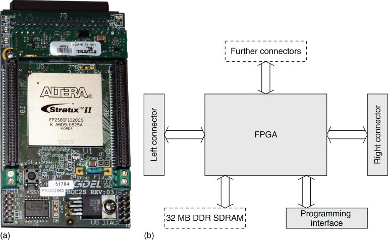
Figure 17.6 (a) A photo of the FPGA board. On the back side (not visible in the photo) further connectors are mounted [10]. (b) A sketch of the main components and connections of the FPGA board. The dashed parts are not used in this application. The programming interface allows a reconfiguration (programming) of the FPGA by an external PC. However, this is used for development only. To use the module (especially stand-alone), at power-up, a pre-preprogrammed configuration is loaded into the FPGA.

The second board of the FPGA-camera module is attached via two of the FPGA board connectors. It holds an application-specific circuit to add the missing components needed for the motion detection application. These components are (1) a CMOS camera, (2) a digital-to-analog converter (DAC), and (3) user interface and serial interface components. The board is depicted in Figure 17.7.

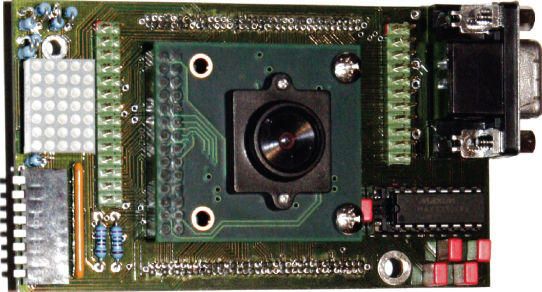
Figure 17.7 Photo of the extension board (front view). On the left-hand side the dot-matrix display and the DIP switch serving as a simple user interface can be seen. The camera module is mounted in the center. On the right-hand side the serial interface components are located. The DAC is mounted below the camera module [10].

The CMOS camera is a Kodak KAC-9630. This is a high-speed camera with 127×100 pixels and a maximum frame rate of 580 fps. The selection of a low-resolution but high-speed camera type is for the purpose of mimicking (up to some degree) the properties of insect vision. The number of ommatidia in insects range from some hundreds (e.g., common fruit fly Drosophila melanogaster: 700) up to some thousands. The spatial resolution (inter-ommatidia angle) can vary from tens of degrees down to, for example, an ommatidia angle of 0.24 in the acute zone in the dragonfly Anax junius [5]. Together with the properties of the (exchangeable) lens (horizontal angle of view of 40), both the number of camera pixels and the inter-pixel angle of 0.315 are appropriate for most insect species.

With the four-channel digital-to-analog converter, an analog output of four independent motion detector arrays can be generated. Details are given in the following section. A simple user interface allows changing of the main settings and display of currently selected modes and important parameters such as brightness setting. Further settings, parameter output, and detector output are accessible via a serial interface.

The components of the whole setup are sketched in Figure 17.8(a). A second camera could be attached at an extra connector. The whole module can be seen in Figure 17.8(b).

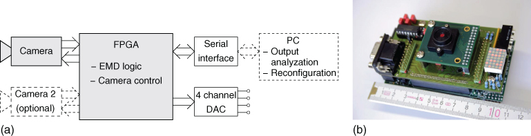
Figure 17.8 (a) A schematic of the EMD module (both boards). The dashed components are not part of the module and need to be attached via the extension board connectors. The main components are shaded. (b) A photo of the whole EMD module (camera side, ruler units are cm) [11]. © IOP Publishing. Reproduced by permission of IOP Publishing. All rights reserved.

17.5.2 A Configurable Array of EMDs

The motion detection computation is carried out by the FPGA. A schematic of the configured FPGA-design is shown in Figure 17.9. The two components “camera controller” and “IC driver” (in the figure on left-hand side) allow a manual or automatic setting of camera parameters, that is, the integration time and the analog camera gain.

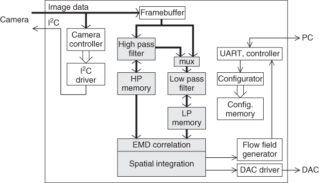
Figure 17.9 The core functionality of the EMD camera module is implemented inside the FPGA. The main FPGA-internal function blocks are shown in this schematic. Thick arrows indicate high bandwidth (image) data. Shaded components realize the EMD computation itself adapted from Ref. [11]. ©IOP Publishing. Reproduced by permission of IOP Publishing. All rights reserved.

The components realizing the actual EMD-array computation are depicted in the center of the figure. This computation is basically sequential, with the EMDs being updated one after the other. However, the computations are carried out in a pipeline (from top to bottom in the figure) parallelizing the lowpass filter, highpass-filter, correlation, and integration in dedicated parts of the FPGA. The pixel data stream from the camera is sampled in a framebuffer. Subsequently, the filter updates are computed. The new filter output values (stored in “HP memory” and “LP memory”) of the two “half-detectors” are correlated and their difference is calculated and summed up for the whole EMD array.

The integration result is (on the right in Figure 17.9) fed to (1) an analog output channel and (2) the serial interface components. Depending on the selected mode, current detector responses are sent out via the serial interface. Alternatively, camera images or other processing results can be transmitted, for example, to an attached PC.

Independent detector responses are accessible via the four analog output channels. Each detector can be supplied with EMD responses of the whole field of view or just a part of it. The camera images are separated into 5 × 5 sub-images (see Figure 17.10(a)) for this purpose. For each subimage, up to 24 × 20 EMDs are computed. The preferred detection direction for each of the 5 × 5 subarrays can be configured in one of eight 45-steps or “off.” Thereby, each of the four detectors can be configured as, for example, a horizontal/vertical/diagonal linear motion detector or as a detector for complex motion types as sketched in Figure 17.5 (e.g., rolling or looming optical flow).

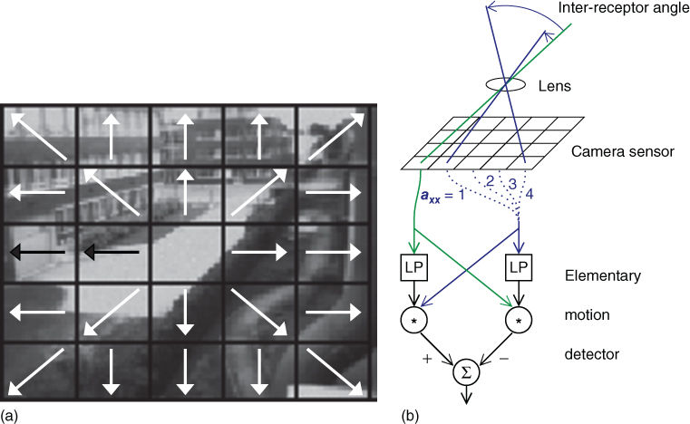
Figure 17.10 (a) A photo taken by the EMD camera module and supplemented by the visualization of an EMD array configuration example (looming detector). (b) The effect of the inter-receptor spacing. The parameter is adjustable in the range from (EMD inoperable) to . The corresponding inter-receptor angle depends on the installed lens [11]. © IOP Publishing. Reproduced by permission of IOP Publishing. All rights reserved.

As described in Section 17.3 the optical parameters of the compound eyes of different species vary a lot. Different inter-ommatidia angles are especially relevant for motion detection as they determine the (minimum) inter-receptor angle of EMDs in the different species. To allow tests with EMDs with different inter-receptor angles, a parameter (called inter-receptor spacing ) is adjustable in this EMD-camera module. The effect of the parameter is depicted in Figure 17.10(b).

Further configurable options are the lowpass filter and highpass filter time constants and the EMD type (n-Ln-, H-Ln-, n-LH-EMD, see caption of Figure 17.3). The camera parameters (integration time, gain) and the EMD update rate can be changed, too. Finally, the output via the serial interface can be selected, for example, EMD array output, image data, flowfield data. The latter produces a two-dimensional optical flow vector per 5×5 subimage.

The measured power consumption of the whole module is in a range of 1–2 W. The higher consumption was generated with a special FPGA configuration having several features, which especially used the DDR memory. A standard design without external memory but with most of the features and running at an update rate of 100 Hz (camera frame rate 100 fps, which is also usable in darker indoor environments) led to the measurement of around 1 W.

This is a relatively low consumption caused by using an FPGA-based design with a rather slow-clocked pipeline design. The camera data is read at a rate of 10 MHz what determines the (slow) speed of the whole pipeline. Because of the EMD-serial computation, only a small part of the FPGA is used (13% of the FPGA logic resources).

17.6 Experimental Results

In this section, experimental results of the presented FPGA-based implementation are shown. The purpose is to show the general behavior of the module. More elaborate and extensive test results can be found in Ref. [10]. There, for example, variations of all parameters are also discussed.

Two test setups were chosen. In the first one, the response of a simple, single-direction, sensitive EMD array to a linear optical flow in the “preferred” detection direction is studied. In this setup, a printed sine pattern was placed in front of the EMD camera module. The module was mounted on a gantry crane with four degrees of freedom: three translatory axes (, , ) and one rotatory axis (around the axis). In the first setup the crane moved only along one translatory axis. The motion axis was in parallel to the sine gradient of the test pattern (and in parallel to the “preferred” detection of the EMD array).

With constant motion speed, the response of the EMD array is also constant. This can be seen in Figure 17.11(a) where the responses for different motion velocities ( axis of the plot) are given. The variation of the motion detector response (minimum and maximum values are given for each velocity) is caused by the practical setup (especially motion speed deviation and illumination differences over the whole pattern). The theoretical EMD responses (with adapted amplitude) are also given in the figure.

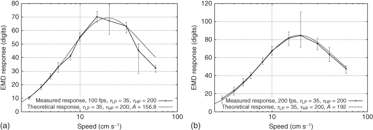
Figure 17.11 Results of the first test setup. In both plots, EMD array responses of several runs are shown. In each run, the camera module was moved linearly with constant speed in front of the test pattern (see text). The motion velocity was changed from run to run. The average, minimum, and maximum EMD array responses are given in the plots for the chosen velocity. The average EMD response is plotted as a solid curve over the motion speed (-axis in log scale). The EMD camera module was configured as a Harris–O'Carroll detector with a lowpass time constant of ms and a highpass time constant of ms. In addition, the theoretically expected responses are plotted as dashed curves [as derived by Borst et al. [15]]. A free amplitude parameter is manually adapted to the measurement data. Therefore, just the curve's shape, peak position, and the relative values – not the absolute ones – can be evaluated. (a) In the plot, the frame rate has been set to fps. (b) A frame rate of fps has been chosen. © IOP Publishing. Reproduced by permission of IOP Publishing. All rights reserved.

In the runs used for the data presented in Figure 17.11(a) the framerate of the camera was set to 100 fps. In the second plot, Figure 17.11(b), responses are shown of runs with an increased framerate of 200 fps. As can be seen, the strong diversion between theoretical and measured responses for the higher velocities in Figure 17.11(a) are not measurable with 200 fps framerate. This indicates an effect of aliasing.

In the second test setup, the EMD camera module was moved along all four axes of the gantry crane (separately, one axis after the other, see Figure 17.12(a)). As test pattern, a checkerboard was used this time. The input image of the test pattern can be seen in Figure 17.12(b). Another difference between the first and the second test setup is the configuration of the EMD array under test. While in the first test only one simple linear detector field was configured and tested, in the second setup, four different EMD array configurations were tested in parallel. The four configurations were (1) a linear vertical detector field, (2) a horizontal detector, (3) a looming detector, and (4) a rotation detector field (see Figure 17.13(a)). The motions carried out by the gantry crane can be recognized by the axes' velocities plotted in Figure 17.12(a).

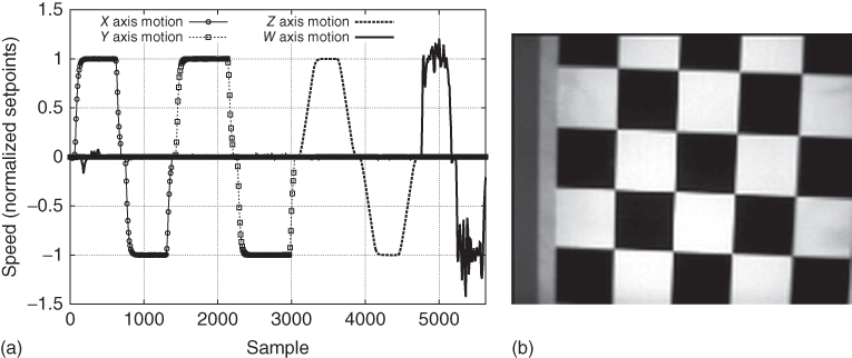
Figure 17.12 (a) The plot shows the motion speed of the four gantry axes in the second test. The data was generated during the same run as used for the data plotted in Figure 17.13(b). The x-, y-, and z-axes of the gantry are parallel to the camera image's vertical, horizontal, and optical axes, respectively. The w-axis of the gantry is parallel to the camera's optical axis. (b) This shows an image of the printed checkerboard test pattern taken by the camera of the EMD module. The integration time and analog gain of the camera were chosen to get a high contrast (both figures taken from Refs [10, 11]). See text and Figure 17.13 for further details. ©IOP Publishing. Reproduced by permission of IOP Publishing. All rights reserved.

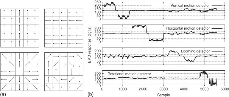
Figure 17.13 (a) The configured preferred directions of the four detectors used in the second test setup are shown (vertical, horizontal, looming, and rotational). (b) The EMD output of the four simultaneously computing detectors during the second test can be seen (both figures taken from Refs [10, 11]). Different movement patterns relative to a checkerboard (Figure 17.12(b)) were carried out sequentially (Figure 17.12(a)). First, there was a vertical translation, followed by a horizontal translation. The third pattern was generated by moving toward and away from the checkerboard (looming) and the last movement pattern corresponded to a rotation around the optical axis. The four detectors selectively respond to their preferred movement pattern and respond only weakly or not at all to their non-preferred patterns. See text and Figure 17.12 for further details. © IOP Publishing. Reproduced by permission of IOP Publishing. All rights reserved.

The responses of the four EMD arrays are shown in Figure 17.13(b). Basically, the response of the four detector fields is the strongest to the motion that generates their preferred optical flow. During the motion, the response can vary with the pattern (see the vertical detector response which depends on the number of horizontal edges visible in the camera image). Furthermore, the response can vary depending on the motion speed (compare Figure 17.13(b) and Figure 17.12(a) for the rotation part).

17.7 Discussion

The FPGA-based EMD camera module presented was designed as a versatile motion detection module for robotic applications, as well as for biological experiments. Hence, the number of EMDs needs to be high enough, the EMD parameters and the array parameters need to be adaptable, and the module needs to be usable stand-alone. Especially compared to previous publications (see Section 17.4.1) these conditions are met very well.

While the number of EMDs per array in the solution described above (and proposed in Ref. [11]) is less than in the setup presented in Ref. [3], the power consumption is also lower. Furthermore, the focus of the module described in this chapter differs from the design in Ref. [3]. As described above, versatility was one main “must” here: being able to switch online between different types of EMD, different time constants, and different preferred flow fields for the four EMD arrays. As shown in Section 17.6, the general detection behavior is as expected for the EMDs and choosing different configurations is also possible.

The comparison of the two designs proposed in Refs [3] and [11] shows very well the advantages and the possibilities of FPGA-based implementations. Depending on the application, a design can be optimized for speed and computational power, for example, with several parallel processing units running at high frequencies. Alternatively, an FPGA design can be optimized for a low power consumption (given a minimum computational power needed for the application). For example, the design shown in Figure 17.9 uses a pipeline structure with parallel computation of the filters. However, the EMDs are computed serially one after the other. Thanks to the optimized computation within the pipeline (as it is possible within an FPGA), the overall computation speed is still enough for computing the whole array serially before the next frame data needs to be computed. The gain from this design is that only 13% of the available FPGA logic elements and only 39% of FPGA-internal memory is used. Therefore, the module consumes only 1–2 W of power.

17.8 Conclusion

In this chapter, mobile robotics was introduced as an application field of bioinspired computer vision methods. In many robotic applications, the resources available for the computer vision task are limited. Most often, the limitations are given in power consumption, space, and/or weight. As could be shown in this chapter, choosing a biologically inspired method can be a solution to meeting such requirements. Some of the tasks to be accomplished by amobile robot have also to be solved in biology (e.g., by an insect). Further, quite often the solution found in biology is also very limited in resource consumption.

Also discussed in this chapter were different ways of implementing biologically inspired methods. As chosen for the implementation presented here, FPGAs combine several advantages. Using FPGAs for the implementation of a biologically inspired computer vision method can lead to a close-to-optimum solution with a good trade-off between effort and costs on the one hand and achieved performance, low power consumption, size, and weight, on the other.

Some more details of the implementation and tests presented here can be found in the publications by Koehler et al. [11] and [10]. Köhler [10] also describes an FPAA-based implementation of EMD and gives a comparison of different implementation methods.

Acknowledgments

The author would like to thank Ralf Möller and the Computer Engineering Group at Bielefeld University, Germany for their support while carrying out most of the design and experiment work presented in this chapter. A special thank goes to Frank Röchter for the work carried out as part of his Diploma thesis and to Jens P. Lindemann for his support in biologically related questions.

Furthermore, the author would like to thank Frank Kirchner and the Robotics Innovation Center (RIC) of the German Research Center for Artificial Intelligence (DFKI) for their support while writing this chapter.

In Section 17.5, an implementation developed in multiple Diploma and Bachelor theses of different authors and further work by the author (all at the Computer Engineering Group at Bielefeld University, Germany) is presented. Further tests were carried out at the Robotics Innovation Center (RIC) at the German Research Center of Artificial Intelligence (DFKI). Parts of this work have been published in Refs [10] and [11]. Thanks to IOP Publishing and to the Andere Verlag for giving their agreement. For these parts: © IOP Publishing. Reproduced by permission of IOP Publishing. All rights reserved.

References

1. 1. Aubepart, F., Farji, M.E., and Franceschini, N. (2004) FPGA implementation of elementary motion detectors for the visual guidance of micro-air-vehicles. 2004 IEEE International Symposium on Industrial Electronics, vol. 1, pp. 71–76.

2. 2. Aubépart, F. and Franceschini, N. (2007) Bio-inspired optic flow sensors based on FPGA: application to micro-air-vehicles. Microprocess. Microsyst., 31, 408–419, doi: http://dx.doi.org/10.1016/j.micpro.2007.02.004, special Issue on Sensor Systems.

3. 3. Plett, J. et al. (2012) Bio-inspired visual ego-rotation sensor for MAVs. Biol. Cybern., 106, 51–63, doi: 10.1007/s00422-012-0478-6.

4. 4. Hassenstein, B. and Reichardt, W. (1956) Systemtheoretische Analyse der Zeit-, Reihenfolgen-, und Vorzeichenauswertung bei der Bewegungsperzeption des Rüsselkäfers Chlorophanus. Z. Naturforsch., 11 (9-10), 513–524.

5. 5. Land, M.F. (1997) Visual acuity in insects. Annu. Rev. Entomol., 42, 147–177.

6. 6. Duke-Elder, S.S. (1958) System of Ophthalmology, The C.V. Mosby Company, St. Louis, MO.

7. 7. Borst, A. and Haag, J. (1996) The intrinsic electrophysiological characteristics of fly lobula plate tangential cells: I. Passive membrane properties. J. Comput. Neurosci., 3 (4), 313–336.

8. 8. Egelhaaf, M. (2006) The neural computation of visual motion information, in Invertebrate Vision, Chapter 10 (eds E. Warrant and D.-E. Nilsson), Cambridge University Press, pp. 399–461.

9. 9. Reichardt, W. (1961) Autocorrelation, a principle for the evaluation of sensory information by the central nervous system, in Sensory Communication (ed. W.A. Rosenblith), MIT Press, New York, pp. 303–317.

10.10. Köhler, T. (2009) Analog and Digital Hardware Implementations of Biologically Inspired Algorithms in Mobile Robotics, Der Andere Verlag.

11.11. Köhler, T. et al. (2009) Bio-inspired motion detection in an FPGA-based smart camera module. Bioinspiration Biomimetics, 4 (1), 015008.

12.12. Egelhaaf, M. and Borst, A. (1989) Transient and steady-state response properties of movement detectors. J. Opt. Soc. Am. A, 6 (1), 116–126.

13.13. Harris, R.A., O'Carroll, D.C., and Laughlin, S.B. (1999) Adaptation and the temporal delay filter of fly motion detectors. Vision Res., 39 (16), 2603–2613.

14.14. Harris, R.A. and O'Carroll, D.C. (2002) Afterimages in fly motion vision. Vision Res., 42 (14), 1701–1714.

15.15. Borst, A., Reisenman, C., and Haag, J. (2003) Adaptation of response transients in fly motion vision. II: model studies. Vision Res., 43 (11), 1309–1322.

16.16. Kirschfeld, K. (1972) The visual system of Musca: studies on optics, structure and function, in Information Processing in the Visual Systems of Arthropods (ed. R. Wehner), Springer-Verlag, Berlin, Heidelberg, New York, pp. 61–74.

17.17. Babies, B. et al. (2011) Contrast-independent biologically inspired motion detection. Sensors, 11, 3303–3326.

18.18. Lindemann, J.P. et al. (2005) On the computations analyzing natural optic flow: quantitative model analysis of the blowfly motion vision pathway. J. Neurosci., 25, 6435–6448, doi: 10.1523/JNEUROSCI.1132-05.2005.

19.19. Franz, M.O. and Krapp, H.G. (2000) Wide-field, motion sensitive neurons and matched filters for optic flow fields. Biol. Cybern., 83, 185–197.

20.20. Zanker, J.M. and Zeil, J. (2002) An analysis of the motion signal distributions emerging from locomotion through a natural environment, in Biologically Motivated Computer Vision: Second International Workshop, BMCV 2002, Tübingen, Germany, November 22-24, 2002. Proceedings, vol. 2525/2002 (eds H. Bulthoff, S.-W. Lee, T. Poggio, and C. Wallraven), Springer-Verlag GmbH, pp. 146–156.

21.21. Ruffier, F. et al. (2003) Bio-inspired optical flow circuits for the visual guidance of micro air vehicles. Proceedings of the 2003 International Symposium on Circuits and Systems, 2003. ISCAS '03, vol. 3 (III), pp. 846–849.

22.22. Harrison, R.R. (2000) An analog VLSI motion sensor based on the fly visual system. PhD thesis, California Institute of Technology, Pasadena, CA, http://www.ece.utah.edu/∼harrison/thesis.pdf(accessed 14 May 2015).

23.23. Harrison, R.R. (2004) A low-power analog VLSI visual collision detector, in Advances in Neural Information Processing Systems, vol. 16 (eds S. Thrun, L. Saul, and B. Scholkopf), MIT Press, Cambridge, MA.

24.24. Harrison, R.R. (2005) A biologically inspired analog IC for visual collision detection. IEEE Trans. Circ. Syst., 52 (11), 2308–2318.

25.25. Franceschini, N., Pichon, J., and Blanes, C. (1992) From insect vision to robot vision. Philos. Trans. R. Soc. London, Ser. B, 337 (1281), 283–294.

26.26. Zhang, T. et al. (2008) An FPGA implementation of insect-inspired motion detector for high-speed vision systems. IEEE International Conference on Robotics and Automation (ICRA), Pasadena, CA, pp. 335–340.

¹ The motion detection described here is done visually, that is, an optical flow is actually detected. Although this optical flow is sometimes (especially in experimental setups) generated just visually without any motion, the method and its application is often referred to as motion detection.