Computer Vision: Models, Learning, and Inference (2012)

In this chapter, we model the relationship between a multidimensional set of measurements {x_n}^N_{n = 1} and an associated multidimensional world state{w_n}^N_{n = 1}. When N is large, it is not practical to describe the full set of dependencies between all of these variables, as the number of model parameters will be too great. Instead, we construct models where we only directly describe the probabilistic dependence between variables in small neighborhoods. In particular, we will consider models in which the world variables {w_n}^N_{n = 1} are structured as chains or trees.

We define a chain model to be one in which the world state variables {w_n}^N_{n = 1} are connected to only the previous variable and the subsequent variable in the associated graphical model (as in Figure 11.2). We define a tree modelto be one in which the world variables have more complex connections, but so there are no loops in the resulting graphical model. Importantly, we disregard the directionality of the connections when we assess whether a directed model is a tree. Hence, our definition of a tree differs from the standard computer science usage.

We will also make the following assumptions:

• The world states w_n are discrete.

• There is an observed data variable x_n associated with each world state w_n.

• The n^th data variable x_n is conditionally independent of all other data variables and world states given the associated world state w_n.

These assumptions are not critical for the development of the ideas in this chapter but are typical for the type of computer vision applications that we consider. We will show that both maximum a posteriori and maximum marginals inference are tractable for this subclass of models, and we will discuss why this is not the case when the states are not organized as a chain or a tree.

To motivate these models, consider the problem of gesture tracking. Here, the goal is to automatically interpret sign language from a video sequence (Figure 11.1). We observe N frames {x_n}^N_n=1 of a video sequence and wish to infer the N discrete variables {w_n}^N_n=1 that encode which sign is present in each of the N frames. The data at time n tells us something about the sign at time n but may be insufficient to specify it accurately. Consequently, we also model dependencies between adjacent world states: we know that the signs are more likely to appear in some orders than others and we exploit this knowledge to help disambiguate the sequence. Since we model probabilistic connections only between adjacent states in the time series, this has the form of a chain model.

Figure 11.1 Interpreting sign language. We observe a sequence of images of a person using sign language. In each frame we extract a vector x_n describing the shape and position of the hands. The goal is to infer the sign w_n that is present. Unfortunately, the visual data in a single frame may be ambiguous. We improve matters by describing probabilistic connections between adjacent states w_n and w_n−1. We impose knowledge about the likely sequence of signs, and this helps disambiguate any individual frame. Images from Purdue RVL-SLLL ASL database (wilbur and Kak 2006).

11.1 Models for chains

In this section, we will describe both a directed and an undirected model for describing chain structure and show that these two models are equivalent.

11.1.1 Directed model for chains

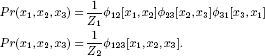
The directed model describes the joint probability of a set of continuous measurements {x_n}^N_n=1 and a set of discrete world states {w_n}^N_n=1 with the graphical model shown in Figure 11.2a. The tendency to observe the measurements x_n given that state w_n takes value k is encoded in the likelihood Pr(x_n|w_n=k). The prior probability of the first state w₁ is explicitly encoded in the discrete distribution Pr(w₁), but for simplicity we assume that this is uniform and omit it from most of the ensuing discussion. The remaining states are each dependent on the previous one, and this information is captured in the distribution Pr(w_n|w_n−1). This is sometimes termed the Markov assumption.

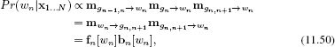
Hence, the overall joint probability is

This is known as a hidden Markov model (HMM). The world states {w_n}^N_n=1 in the directed model have the form of a chain, and the overall model has the form of a tree. As we shall see, these properties are critical to our ability to perform inference.

11.1.2 Undirected model for chains

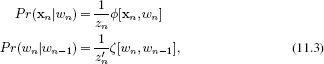
The undirected model (see Section 10.3) describes the joint probability of the measurements {x_n}^N_n=1 and the world states {w_n}^N_n=1 with the graphical model shown in Figure 11.2b. The tendency for the measurements and the data to take certain values is encoded in the potential function [x_n, w_n]. This function always returns positive values and returns larger values when the measurements and the world state are more compatible. The tendency for adjacent states to take certain values is encoded in a second potential function ζ[w_n, w_n−1] which returns larger values when the adjacent states are more compatible. Hence, the overall probability is

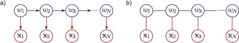
Figure 11.2 Models for chains. a) Directed model. There is one observation variable x_n for each state variable w_n and these are related by the conditional probability Pr(x_n|w_n) (downward arrows). Each state w_n is related to the previous one by the conditional probability Pr(w_n|w_n−1)(horizontal arrows). b) Undirected model. Here, each observed variable x_n is related to its associated state variable w_n via the potential function [x_n, w_n] and the neighboring states are connected via the potential function ζ[w_n, w_n−1].

Once more the states form a chain and the overall model has the form of a tree; there are no loops.

11.1.3 Equivalence of models

When we take a directed model and make the edges undirected, we usually create a different model. However, comparing Equations 11.1 and 11.2 reveals that these two models represent the same factorization of the joint probability density; in this special case, the two models are equivalent. This equivalence becomes even more apparent if we make the substitutions

where z_n and z′_n are normalizing factors which form the partition function:

Since the directed and undirected versions of the chain model are equivalent, we will continue our discussion in terms of the directed model alone.

11.1.4 Hidden Markov model for sign language application

We will now briefly describe how this directed model relates to the sign language application. We preprocess the video frame to create a vector x_n that represents the shape of the hands. For example, we might just extract a window of pixels around each hand and concatenate their RGB pixel values.

We now model the likelihood Pr(x_n|w_n=k) of observing this measurement vector given that the sign w_n in this image takes value k. A very simple model might assume that the measurements have a normal distribution with parameters that are contingent on which sign is present so that

We model the sign w_n as a being categorically distributed, where the parameters depend on the previous sign w_n−1 so that

This hidden Markov model has parameters {μ_k,∑_k,λ_k}^K_k=1. For most of this chapter, we will assume that these parameters are known, but we return briefly to the issue of learning in Section 11.6. We now turn our focus to inference in this type of model.

11.2 MAP inference for chains

Consider a chain with N unknown variables {w_n}^N_n=1, each of which can take K possible values. Here, there are K^N possible states of the world. For real-world problems, this means that there are far too many states to evaluate exhaustively; we can neither compute the full posterior distribution nor search directly through all of the states to find the maximum a posteriori estimate.

Fortunately, the factorization of the joint probability distribution (the conditional independence structure) can be exploited to find more efficient algorithms for MAP inference than brute force search. The MAP solution is given by

where line 2 follows from Bayes’ rule. We have reformulated this as a minimization problem in line 3.

Substituting in the expression for the log probability (Equation 11.1), we get

which has the general form

where U_n is a unary term and depends only on a single variable w_n and P_n is a pairwise term, depending on two variables w_n and w_n−1. In this instance, the unary and pairwise terms can be defined as

Any problem that has the form of Equation 11.9 can be solved in polynomial time using the Viterbi algorithm which is an example of dynamic programming.

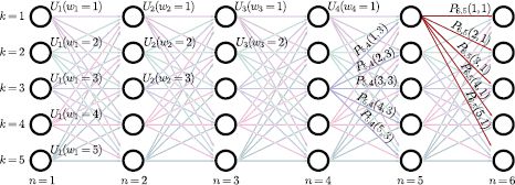
Figure 11.3 Dynamic programming formulation. Each solution is equated with a particular path from left-to-right through an acyclic directed graph. The N columns of the graph represent variables w₁… N and the K rows represent possible states 1… K. The nodes and edges of the graph have costs associated with the unary and pairwise terms, respectively. Any path from left to right through the graph has a cost that is the sum of the costs at all of the nodes and edges that it passes through. Optimizing the function is now equivalent to finding the path with the least cost.

11.2.1 Dynamic programming (Viterbi algorithm)

To optimize the cost function in Equation 11.9, we first visualize the problem with a 2D graph with vertices . The vertex V_n, _k represents choosing the k^th world state at the n^th variable (Figure 11.3). Vertex V_n,_k is connected by a directed edge to each of the vertices {V_n+1, _k)^K_k=1 at the next pixel position. Hence, the organization of the graph is such that each valid horizontal path from left to right represents a possible solution to the problem; it corresponds to assigning one value k ∈ [1…K] to each variable w_n.

We now attach the costs U_n(w_n=k) to the vertices V_{n, k}. We also attach the costs Pn(w_n=k, w_n−1=l) to the edges joining vertices V_{n−1, l} to V_n, _k. We define the total cost of a path from left to right as the sum of the costs of the edges and vertices that make up the path. Now, every horizontal path represents a solution and the cost of that path is the cost for that solution; we have reformulated the problem as finding the minimum cost path from left to right across the graph.

Finding the minimum cost

The approach to finding the minimum cost path is simple. We work through the graph from left to right, computing at each vertex the minimum possible cumulative cost S_n, _k to arrive at this point by any route. When we reach the right-hand side, we compare the K values S_N,• and choose the minimum. This is the lowest possible cost for traversing the graph. We now retrace the route we took to reach this point, using information that was cached during the forward pass.

The easiest way to understand this method is with a concrete example (Figures 11.4 and 11.5) and the reader is encouraged to scrutinize these figures before continuing.

A more formal description is as follows. Our goal is to assign the minimum possible cumulative cost S_n, _k for reaching vertex V_n, _k. Starting at the left-hand side, we set the first column of vertices to the unary costs for the first variable:

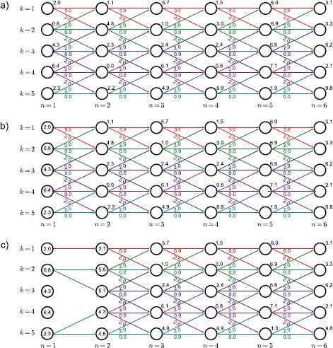
Figure 11.4 Dynamic programming. a) The unary cost U_n(w_n=k) is given by the number above and to the right of each node. The pairwise costs P_n(w_n, w_n−1) are zero if w_n=w_n−1 (horizontal), two if |w_n−w_n−1|=1, and ∞ otherwise. This favors a solution that is mostly constant but can also vary smoothly. For clarity, we have removed the edges with infinite cost as they cannot become part of the solution. We now work from left to right, computing the minimum cost S_n,k for arriving at vertex V_n,k by any route. b) For vertices {V_1,k}^K_{k = 1}, the minimum cost is just the unary cost associated with that vertex. We have stored the values S_1,1…S_1,5 inside the circle representing the respective vertex. c) To compute the minimum cost S_2,1 at vertex (n=2, k=1), we must consider two possible routes. The path could have traveled horizontally from vertex (1,1) giving a total cost of 2.0+0.0+1.1=3.1, or it may have come diagonally upward from vertex (1,2) with cost 0.8+2.0+1.1=3.9. Since the former route is cheaper, we use this cost, store S_2,1=3.1 at the vertex, and also remember the path used to get here. Now, we repeat this procedure at vertex (2,2) where there are three possible routes from vertices (1,1), (1,2) and (1,3). Here it turns out that the best route is from (1,2) and has total cumulative cost of S_2,2 = 5.6. Example continued in Figure 11.5.

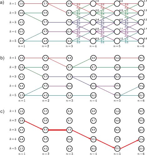
Figure 11.5 Dynamic programming worked example (continued from Figure 11.4). a) Having updated the vertices at pixel n=2, we carry out the same procedure at pixel n=3, accumulating at each vertex the minimum total cost to reach this point. b) We continue updating the minimum cumulative costs S_n,k to arrive at pixel n in state k until we reach the right hand side. c) We identify the minimum cost among the right-most vertices. In this case, it is vertex (6,4), which has cost S_6,4=17.4. This is the minimum possible cost for traversing the graph. By tracing back the route that we used to arrive here (red arrows), we find the world state at each pixel that was responsible for this cost.

The cumulative total S_2,k for the k^th vertex in the second column should represent the minimum possible cumulative cost to reach this point. To calculate this, we consider the K possible predecessors and compute the cost for reaching this vertex by each possible route. We set S_2,k to the minimum of these values and store the route by which we reached this vertex so that

More generally, to calculate the cumulative totals S_n,k, we use the recursion

and we also cache the route by which this minimum was achieved at each stage. When we reach the right-hand side, we find the value of the final variable w_n that minimizes the total cost

and set the remaining labels {_n}^N−1_n=1 according to the route that we followed to get to this value.

This method exploits the factorization structure of the joint probability between the observations and the states to make vast computational savings. The cost of this procedure is (NK²), as opposed to (K^N) for a brute force search through every possible solution.

11.3 MAP inference for trees

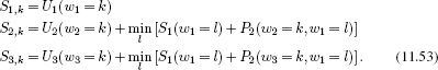
To show how MAP inference works in tree-structured models, consider the model in Figure 11.6. For this graph, the prior probability over the states factorizes as

and the world states have the structure of a tree (disregarding the directionality of the edges).

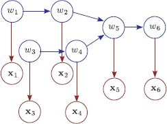
Figure 11.6 Tree-based models. As before, there is one observation x_n for each world state w_n, and these are related by the conditional probability Pr(x_n|w_n). However, disregarding the directionality of the edges, the world states are now connected as a tree. Vertex w₅ has two incoming connections, which means that there is a ‘three-wise’ term Pr(w₅|w₂, w₄) in the factorization. The tree structure means it is possible to perform MAP and max-marginals inference efficiently.

Once more, we can exploit this factorization to compute the MAP solution efficiently. Our goal is to find

By a similar process to that in Section 11.2, we can rewrite this as a minimization problem with the following cost function:

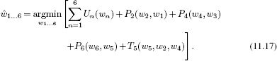
As before, we reformulate this cost function in terms of finding a route through a graph (see Figure (see Figure 11.7). The unary costs U_n are associated with each vertex. The pairwise costs P_m are associated with edges between pairs of adjacent vertices. The three-wise cost T₅ is associated with the combination of states at the point where the tree branches. Our goal now is to find the least cost path from all of the leaves simultaneously to the root.

We work from the leaves to the root of the tree, at each stage computing S_n,k, the cumulative cost for arriving at this vertex (see worked example in Figure 11.7). For the first four vertices, we proceed as in standard dynamic programming:

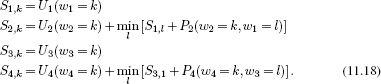
When we come to the branch in the tree, we try to find the best combination of routes to reach the nodes for variable 5; we must now minimize over both variables to compute the next term. In other words,

Finally, we compute the last terms as normal so that

Now we find the world state associated with the minimum of this final sum and trace back the route that we came by as before, splitting the route appropriately at junctions in the tree.

Dynamic programming in this tree has a greater computational complexity than dynamic programming in a chain with the same number of variables as we must minimize over two variables at the junction in the tree. The overall complexity is proportional to K^W, where W is the maximum number of variables over which we must minimize.

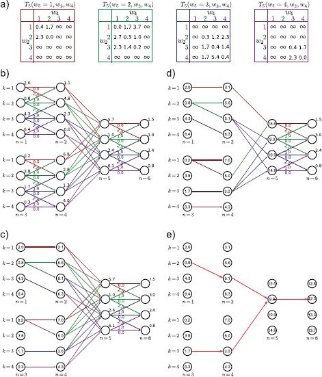
Figure 11.7 Dynamic programming example for tree model in Figure 11.6. a) Table of three-wise costs at vertex 5. This is a K×K×K table consisting of the costs associated with Pr(w₅|w₂, w₄). Pairwise costs are as for the example in Figure 11.4. b) Tree-structured model with unary and pairwise costs attached. c) We work from the leaves, finding the minimal possible cost S_n, _k to reach vertex n in state k as in the original dynamic programming formulation. d) When we reach the vertex above a branch (here, vertex 5), we find the minimal possible cost, considering every combination of the incoming states. e) We continue until we reach the root. There, we find the minimum overall cost and trace back, making sure to split at the junction according to which pair of states was chosen.

For directed models, W is equal to the largest number of incoming connections at any vertex. For undirected models, W will be the size of the largest clique. It should be noted that for undirected models, the critical property that allows dynamic programming solutions is that the cliques themselves form a tree (see Figure 11.11).

11.4 Marginal posterior inference for chains

In Section 11.3, we demonstrated that it is possible to perform MAP inference in chain models efficiently using dynamic programming. In this section, we will consider a different form of inference: we will aim to calculate the marginal distribution Pr(w_n|x₁…_N} over each state variable w_n separately.

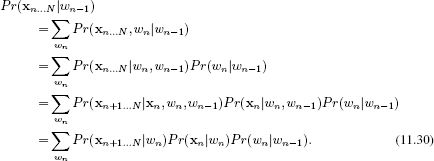
Consider computing the marginal distribution over the variable w_N. By Bayes’ rule we have

The right-hand side of this equation is computed by marginalizing over all of the other state variables except w_N so we have

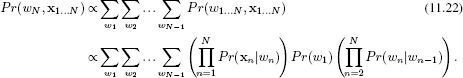
Unfortunately, in its most basic form, this marginalization involves summing over N−1 dimensions of the N dimensional probability distribution. Since this discrete probability distribution contains K^N entries, computing this summation directly is not practical for realistic-sized problems. To make progress, we must again exploit the structured factorization of this distribution.

11.4.1 Computing one marginal distribution

We will first discuss how to compute the marginal distribution Pr(w_N|x₁… _N) for the last variable in the chain w_N. In the following section, we will exploit these ideas to compute all of the marginal distributions Pr(w_n|x₁…_N) simultaneously.

We observe that not every term in the product in Equation 11.22 is relevant to every summation. We can rearrange the summation terms so that only the variables over which they sum are to the right

Then, we proceed from right to left, computing each summation in turn. This technique is known as variable elimination. Let us denote the rightmost two terms as

Then we sum over w₁ to compute the function

At the n^th stage, we compute

and we repeat this process until we have computed the full expression. We then normalize the result to find the marginal posterior Pr(w_N|x₁… _N) (Equation 11.21).

This solution consists of N−1 summations over K values; it is much more efficient to compute than explicitly computing all K^N solutions and marginalizing over N−1 dimensions.

11.4.2 Forward-backward algorithm

In the previous section, we showed an algorithm that could compute the marginal posterior distribution Pr(w_N|x₁…_N) for the last world state w_N. It is easy to adapt this method to compute the marginal posterior Pr(w_n|x₁…_N) over any other variable w_n. However, we usually want all of the marginal distributions, and it is inefficient to compute each separately as much of the effort is replicated. The goal of this section is to develop a single procedure that computes the marginal posteriors for all of the variables simultaneously and efficiently using a technique known as the forward-backward algorithm.

The principle is to decompose the marginal posterior into two terms

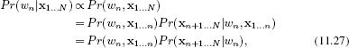
where the relation between the second and third line is true because x_1…n and x_n+1…N are conditionally independent given w_n (as can be gleaned from Figure 11.2). We will now focus on finding efficient ways to calculate each of these two terms.

Forward recursion

Let us consider the first term Pr(w_n,x₁…_n). We can exploit the recursion

where we have again applied the conditional independence relations implied by the graphical model between the last two lines.

The term Pr(w_n, x₁…_n) is exactly the intermediate function f_n[w_n] that we calculated in the solution for the single marginal distribution in the previous section; we have reproduced the recursion

but this time, we based the argument on conditional independence rather than the factorization of the probability distribution. Using this recursion, we can efficiently compute the first term of Equation 11.27 for all n; in fact, we were already doing this in our solution for the single marginal distribution Pr(w_N|x₁…_N).

Backward recursion

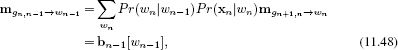
Now consider the second term Pr(x_n+1…N|w_n) from Equation 11.27. Our goal is to develop a recursive relation for this quantity so that we can compute it efficiently for all n. This time the recursion works backwards from the end of the chain to the front, so our goal is to establish an expression for Pr(x_n…N|w_n−1) in terms of Pr(x_n+1…_N|w_n):

Here we have again applied the conditional independence relations implied by the graphical model between the last two lines. Denoting the probability Pr(x_{n + 1}…_N}|w_n) as b_n[w_n], we see that we have the recursive relation

We can use this to compute the second term in Equation 11.27 efficiently for all n.

Forward-backward algorithm

We can now summarize the forward-backward algorithm to compute the marginal posterior probability distribution for all n. First, we observe (Equation 11.27) that the marginal distribution can be computed as

We recursively compute the forward terms using the relation

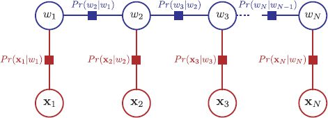
Figure 11.8 Factor graph for chain model. There is one node per variable (circles) and one function node per term in the factorization (squares). Each function node connects to all of the variables associated with this term.

where we set f₁[w₁]=Pr(x₁|w₁)Pr(w₁). We recursively compute the backward terms using the relation

where we set b_N[w_N]to the constant value 1/K.

Finally, to compute the n^th marginal posterior distribution, we take the product of the associated forward and backward terms and Normalize.

11.4.3 Belief propagation

The forward-backward algorithm can be considered a special case of a more general technique called belief propagation. Here, the intermediate functions f[•]and b[•] are considered as messages that convey information about the variables. In this section, we describe a version of belief propagation known as the sum-product algorithm. This does not compute the marginal posteriors any faster than the forward-backward algorithm, but it is much easier to see how to extend it to models based on trees.

The sum-product algorithm operates on a factor graph. A factor graph is a New type of graphical model that makes the factorization of the joint probability more explicit. It is very simple to convert directed and undirected graphical models to factor graphs. As usual, we introduce one Node per variable; for example variables w₁, w₂, and w₃ all have a variable Node associated with them. We also introduce one function node per term in the factorized joint probability distribution; in a directed model this would represent a conditional probability term such as Pr(w₁|w₂, w₃) and in an undirected model it would represent a potential function such as [w₁, w₂}, w₃]. We then connect each function Node to all of the variable nodes relevant to that term with undirected links. So, in a directed model, a term like Pr(x₁|w₁, w₂) would result in a function node that connects to x₁, w₁ and w₂. In an undirected model, a term like ₁₂(w₁, w₂) would result in a function node that connects to w₁ and w₂. Figure 11.8 shows the factor graph for the chain model.

Sum-product algorithm

The sum product algorithm proceeds in two phases: a forward pass and a backward pass. The forward pass distributes evidence through the graph and the backward pass collates this evidence. Both the distribution and collation of evidence are accomplished by passing messages from node to node in the factor graph. Every edge in the graph is connected to exactly one variable node, and each message is defined over the domain of this variable. There are three types of messages:

1. A message from an unobserved variable z_p to a function node g_q is given by

where ne[p] returns the set of the neighbors of z_p in the graph and so the expression ne[p]\q denotes all of the neighbors except q. In other words, the message from a variable to a function node is the pointwise product of all other incoming messages to the variable; it is the combination of other beliefs.

2. A message from an observed variable z_p = z*_p to a function node g_q is given by

In other words, the message from an observed node to a function conveys the certain belief that this node took the observed value.

3. A message from a function node g_p to a recipient variable z_q is defined as

This takes beliefs from all variables connected to the function except the recipient variable and uses the function g_p[•] to convert these to a belief about the recipient variable.

In the forward phase, the message passing can proceed in any order, as long as the outgoing message from any variable or function is not sent until all the other incoming messages have arrived. In the backward pass, the messages are sent in the opposite order to the forward pass.

Finally, the marginal distribution at node z_p can be computed from a product of all of the incoming messages from both the forward and reverse passes so that

A proof that this algorithm is correct is beyond the scope of this book. However, to make this at least partially convincing (and more concrete), we will work through these rules for the case of the chain model (Figure 11.8), and we will show that exactly the same computation occurs as for the forward-backward algorithm.

11.4.4 Sum-product algorithm for chain model

The factor graph for the chain solution annotated with messages is shown in Figure 11.9. We will now describe the sum-product algorithm for the chain model.

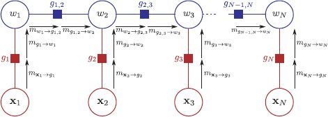
Figure 11.9 Sum product algorithm for chain model (forward pass). The sum-product algorithm has two phases. In the forward phase, messages are passed through the graph in an order such that a message cannot be sent until all incoming messages are receive at the source node. So, the message cannot be sent until the messages and have been received.

Forward pass

We start by passing a message from node x₁ to the function node g₁. Using rule 2, this message is a delta function at the observed value x*₁ so that

Now we pass a message from function g₁ to node w₁. Using rule 3, we have

By rule 1, the message from node w₁ to function g_1,2 is simply the product of the incoming nodes, and since there is only one incoming node, this is just

By rule 3, the message from function g_1,2 to node w₂ is computed as

Continuing this process, the messages from x₂ to g₂ and g₂ to w₂ are

and the message from w₂ to g_2,3 is

A clear pattern is emerging; the message from node w_n to function g_{n, n+1} is equal to the forward term from the forward-backward algorithm:

In other words, the sum-product algorithm is performing exactly the same computations as the forward pass of the forward-backward algorithm.

Backward pass

When we reach the end of the forward pass of the belief propagation, we initiate the backward pass. There is no need to pass messages toward the observed variables x_n since we already know their values for certain. Hence, we concentrate on the horizontal connections between the unobserved variables (i.e., along the spine of the model). The message from node w_N to function g_{N, N−1} is given by

and the message from g_{N, N−1} to w_N−1 is given by

In general, we have

which is exactly the backward recursion from the forward-backward algorithm.

Collating evidence

Finally, to compute the marginal probabilities, we use the relation

and for the general case, this consists of three terms:

where in the second line we have used the fact that the outgoing message from a variable node is the product of the incoming messages. We conclude that the sum-product algorithm computes the posterior marginals in exactly the same way as the forward backward algorithm.

11.5 Marginal posterior inference for trees

To compute the marginals in tree-structured models we simply apply the sum product algorithm to the new graph structure. The factor graph for the tree in Figure 11.6 is shown in Figure 11.10. The only slight complication is that we must ensure that the first two incoming messages to the function relating variables w₂, w₄, and w₅ have arrived before sending the outgoing message. This is very similar to the order of operations in the dynamic programming algorithm.

For undirected graphs, the key property is that the cliques, not the nodes, form a tree. For example, there is clearly a loop in the undirected model in Figure 11.11a, but when we convert this to a factor graph the structure is a tree (Figure 11.11b). For models with only pairwise cliques, the cliques always form a tree if there are no loops in the original graphical model.

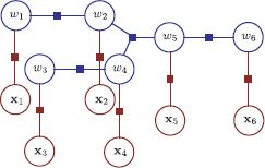
Figure 11.10 Factor graph corresponding to tree model in Figure 11.6. There is one function node connecting each world state variable to its associated measurement and these correspond to the terms Pr(x_n|w_n). There is one function node for each of the three pairwise terms Pr(w₂|w₁), Pr(w₄|w₃) and Pr(w₆|w₅) and this connected to both contributing variables. The function node corresponding to the three-wise term Pr(w₅|w₂, w₄) has three neighbors, w₅, w₂, and w₄.

11.6 Learning in chains and trees

So far, we have only discussed inference for these models. Here, we briefly discuss learning which can be done in a supervised or unsupervised context. In the supervised case, we are given a training set of I matched sets of states and data . In the unsupervised case, we only observe the data

Supervised learning for directed models is relatively simple. We first isolate the part of the model that we want to learn. For example, we might learn the parameters θ of Pr(x_n|w_n, θ) from paired examples of x_n and w_n. We can then learn these parameters in isolation using the ML, MAP, or Bayesian methods.

Unsupervised learning is more challenging; the states w_n are treated as hidden variables and the EM algorithm is applied. In the E-step, we compute the posterior marginals over the states using the forward backward algorithm. In the M-step we use these marginals to update the model parameters. For the hidden Markov model (the chain model), this is known as the Baum-Welch algorithm.

As we saw in the previous chapter, learning in undirected models can be challenging; we cannot generally compute the normalization constant Z and this in turn prevents us from computing the derivative with respect to the parameters. However, for the special case of tree and chain models, it is possible to compute Z efficiently and learning is tractable. To see why this is the case, consider the undirected model from Figure 11.2b, which we will treat here as representing the conditional distribution

since the data nodes {x_n}^N_n=1 are fixed. This model is known as a 1D conditional random field. The unknown constant Z now has the form

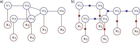
Figure 11.11 Converting an undirected model to a factor graph. a) Undirected model. b) Corresponding factor graph. There is one function node for each maximal clique (each clique which is not a subset of another clique). Although there was clearly a loop in the original graph, there is no loop in the factor graph and so the sum-product algorithm is still applicable.

Figure 11.12 Grid-based models. For many vision problems, the natural description is a grid-based model. We observe a grid of pixel values {x_n}^N_n=1 and wish to infer an unknown world state {w_n}^N_n=1 associated with each site. Each world state is connected to its neighbors. These connections are usually applied to ensure a smooth or piecewise smooth solution. a) Directed grid model. b) Undirected grid model (2D conditional random field).

We have already seen that it is possible to compute this type of sum efficiently, using a recursion (Equation 11.26). Hence, Z can be evaluated and maximum likelihood learning can be performed in this model without the need for contrastive divergence.

11.7 Beyond chains and trees

Unfortunately, there are many models in computer vision that do not take the form of a chain or a tree. Of particular importance are models that are structured to have one unknown w_n for each RGB pixel x_n in the image. These models are naturally structured as grids and the world states are each connected to their four pixel neighbors in the graphical model (Figure 11.12). Stereo vision, segmentation, denoising, superresolution, and many other vision problems can all be framed in this way.

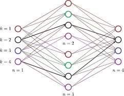
Figure 11.13 Dynamic programming fails when there are undirected loops. Here, we show a 2 × 2 image where we have performed a naïve forward pass through the variables. On retracing the route, we see that the two branches disagree over which state the first variable took. For a coherent solution the cumulative minimum costs at node 4, we should have forced the two paths to have common ancestors. With a large number of ancestors this is too computationally expensive to be practical.

We devote the whole of the next chapter to grid-based problems, but we will briefly take the time to examine why the methods developed in this chapter are not suitable. Consider a simple model based on a 2 × 2 grid. Figure 11.13illustrates why we cannot blindly use dynamic programming to compute the MAP solution. To compute the minimum cumulative cost S_n at each node, we might naïvely proceed as normal:

Now consider the fourth term. Unfortunately,

The reason for this is that the partial cumulative sums S₂ and S₃ at the two previous vertices both rely on minimizing over the same variable w₁. However, they did not necessarily choose the same value at w₁. If we were to trace back the paths we took, the two routes back to vertex one might predict a different answer. To properly calculate the minimum cumulative cost at node S₄, _k, we would have to take account of all three ancestors: the recursion is no longer valid, and the problem becomes intractable once more.

Similarly, we cannot perform belief propagation on this graph: the algorithm requires us to send a message from a node only when all other incoming messages have been received. However, the nodes w₁, w₂, w₃, and w₄ all simultaneously require messages from one another and so this is not possible.

11.7.1 Inference in graphs with loops

Although the methods of this chapter are not suitable for models based on graphs with loops, there are a number of ways to proceed:

1. Prune the graph. An obvious idea is to prune the graph by removing edges until what is left has a tree structure (Figure 11.14). The choice of which edges to prune will depend on the real-world problem.

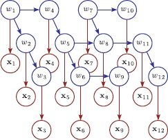
Figure 11.14 Pruning graphs with loops. One approach to dealing with models with loops is simply to prune the connections until the loops are removed. This graphical model is the model from Figure 11.12a after such a pruning process. Most of the connections are retained but now the remaining structure is a tree. The usual approach to pruning is to associate a strength with each edge so that weaker edges are more desirable. Then we compute the minimum spanning tree based in these strengths and discard any connections that do not form part of the tree.

Figure 11.15 Combining variables. a) This graphical model contains loops. b) We form three compound variables, each of which consists of all of the variables in one of the original columns. These are now connected by a chain structure. However, the price we pay is that if there were K states for each original variable, the compound variables now have K³ states.

2. Combine variables. A second approach is to combine variables together until what remains has the structure of a chain or tree. For example, in Figure 11.15 we combine the variables w₁, w₂, and w₃, to make a new variable w₁₂₃and the variables w₄, w₅, and w₆ to form w₄₅₆. Continuing in this way, we form a model that has a chain structure. If each of the original variables had K states, then the compound variables will have K³ states, and so inference will be more expensive. In general the merging of variables can be automated using the junction tree algorithm. Unfortunately, this example illustrates why this approach will not work for large grid models: we must merge together so many variables that the resulting compound variable has too many states to work with.

3. Loopy belief propagation. Another idea is to simply apply belief propagation regardless of the loops. All messages are initialized to uniform and then the messages are repeatedly passed in some order according to the normal rules. This algorithm is not guaranteed to converge to the correct solution for the marginals (or indeed to converge at all) but in practice it produces useful results in many situations.

4. Sampling approaches. For directed graphical models, it is usually easy to draw samples from the posterior. These can then be aggregated to compute an empirical estimate of the marginal distributions.

5. Other approaches: There are several other approaches for exact or approximate inference in graphs, including tree reweighted message passing and graph cuts. The latter is a particularly important class of algorithms, and we devote most of Chapter 12 to describing it.

11.8 Applications

The models in this chapter are attractive because they permit exact MAP inference. They have been applied to a Number of problems in which there are assumed spatial or temporal connections between parts of a model.

11.8.1 Gesture tracking

The goal of gesture tracking is to classify the position {w_n}^N_n=1 of the hands within each of the N captured frames from a video sequence into a discrete set of possible gestures, w_n∈ {1,2,…, K} based on extracted data {x_n}^N_n=1 from those frames. starner et al. (1998) presented a wearable system for automatically interpreting sign language gestures. A camera mounted in the user’s hat captured a top-down view of their hands (Figure 11.16). The positions of the hands were identified by using a per-pixel skin segmentation technique (see Section 6.6.1). The state of each hand was characterized in terms of the position and shape of a bounding ellipse around the associated skin region. The final eight-dimensional data vector x concatenated these measurements from each hand.

To describe the time sequences of these measurements, Starner et al. (1998) developed a hidden Markov model-based system in which the states w_n each represented a part of a sign language word. Each of these words was represented by a progression through four values of the state variable w, representing the various stages in the associated gesture for that word. The progression through these states might last any Number of time steps (each state can be followed by itself so it can cycle indefinitely) but must come in the required order. They trained the system using 400 training sentences. They used a dynamic programming method to estimate the most likely states w and achieved recognition accuracy of 97.8 percent using a 40-word lexicon with a test set of 100 sentences. They found that performance was further improved if they imposed knowledge about the fixed grammar of each phrase (pronoun, verb, Noun, adjective, pronoun). Remarkably, the system worked at a rate of 10 frames a second.

11.8.2 Stereo vision

In dense stereo vision, we are given two images of the same scene taken from slightly different positions. For our purposes, we will assume that they have been preprocessed so that for each pixel in image 1, the corresponding pixel is on the same scanline in image 2 (a process known as rectification; see Chapter 16). The horizontal offset or disparity between corresponding points depends on the depth. Our goal is to find the discrete disparity field w given the observed images x⁽¹⁾ and x⁽²⁾, from which the depth of each pixel can be recovered (Figure 11.17).

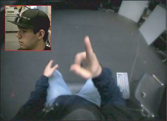
Figure 11.16 Gesture tracking from Starner et al. (1998). A camera was mounted on a baseball cap (inset) looking down at the users hands. The camera image (main figure) was used to track the hands in a HMM-based system that could accurately classify a 40-word lexicon and worked in real time. Each word was associated with four states in the HMM. The system was based on a compact description of the hand position and orientation within each frame. Adapted from Starner et al. (1998),© 1998 Springer.

We assume that the pixel in image 1 should closely resemble the pixel at the appropriate offset (disparity) in image 2 and any remaining small differences are treated as noise so that

where w_m,_n is the disparity at pixel (m,n) of image 1, x⁽¹⁾_m,n is the RGB vector from pixel (m,n) of image 1 and x_m,n⁽²⁾ is the RGB vector from pixel (m,n) of image 2.

Unfortunately, if we compute the maximum likelihood disparities w_m, _n at each pixel separately, the result is extremely noisy (Figure 11.18a). As Figure 11.17 illustrates, the choice of disparity is ambiguous in regions of the image where there are few visual changes. In layman’s terms, if the nearby pixels are all similar, it is difficult to establish with certainty which corresponds to a given position in the other image. To resolve this ambiguity, we introduce a prior Pr(w) that encourages piecewise smoothness in the disparity map; we are exploiting the fact that we know that the scene mainly consists of smooth surfaces, with occasional jumps in disparity at the edge of objects.

One possible approach (attributed originally to Ohta and Kanade 1985) to recovering the disparity is to use an independent prior for each scanline so that

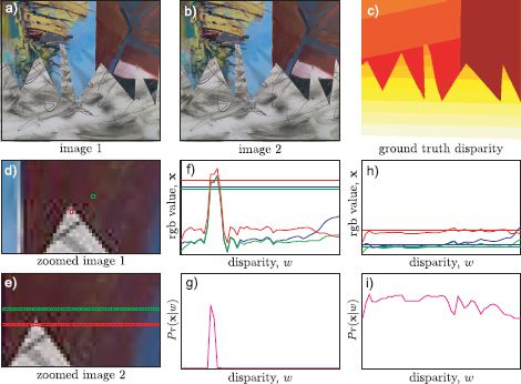
Figure 11.17 Dense stereo vision. a-b) Two images taken from slightly different positions. The corresponding point for every pixel in the first image is somewhere on the same scanline in the second image. The horizontal offset is known as the disparity and is inversely related to depth. c) Ground truth disparity map for this image. d) Close-up of part of first image with two pixels highlighted. e) Close-up of second image with potential corresponding pixels highlighted. f) RGB values for red pixel (dashed lines) in first image and as a function of the position in second image (solid lines). At the correct disparity, there is very little difference between the RGB values in the two images and so g) the likelihood that this disparity is correct is large. h-i) For the green pixel (which is in a smoothly changing region of the image), there are many positions where the RGB values in the second image are similar and hence many disparities have high likelihoods; the solution is ambiguous.

where each scanline was organized into a chain model (Figure 11.2) so that

The distributions Pr(w_{m, n}|w_{m, n−1}) are chosen so that they allot a high probability when adjacent disparities are the same, an intermediate probability when adjacent disparities change by a single value, and a low probability if they take values that are more widely separated. Hence, we encourage piecewise smoothness.

MAP inference can be performed within each scanline separately using the dynamic programming approach and the results combined to form the full disparity field w. Whereas this definitely improves the fidelity of the solution, it results in a characteristic “streaky” result (Figure 11.18b). These artifacts are due to the (erroneous) assumption that the scanlines are independent. To get an improved solution, we should smooth in the vertical direction as well, but the resulting grid-based model will contain loops, making MAP inference problematic.

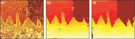
Figure 11.18 Dense stereo results. Recovered disparity maps for a) independent pixels model, b) independent scanlines model, and c) tree-based model of Veksler (2005).

Veksler (2005) addressed this problem by pruning the full grid-based model until it formed a tree. Each edge was characterized by a cost that increased if the associated pixels were close to large changes in the image; at these positions, either there is texture in the image (and so the disparity is relatively well defined) or there is an edge between two objects in the scene. In either case, there is no need to apply a smoothing prior here. Hence, the minimum spanning tree tends to retain edges in regions where they are most needed. The minimum spanning tree can be computed using a standard method such as Prim’s algorithm (see Cormen et al. 2001).

The results of MAP inference using this model are shown in Figure 11.18c. The solution is piecewise smooth in both directions and is clearly superior to either the independent pixels model or the independent scanline approach. However, even this model is an unnecessary approximation; we would ideally like the variables to be fully connected in a grid structure, but this would obviously contain loops. In Chapter 12, we consider models of this sort and revisit stereo vision.

11.8.3 Pictorial Structures

Pictorial structures are models for object classes that consist of a number of individual parts that are connected together by spring-like connections. A typical example would be a face model (Figure 11.19), which might consist of a nose, eyes, and mouth. The spring-like connections encourage the relative positions of these features to take sensible values. For example, the mouth is strongly encouraged to be below the nose. Pictorial structures have a long history in computer vision but were revived in a modern form by Felzenszwalb and Huttenlocher(2005) who identified that if the connections between parts take the form of an acyclic graph (a tree), then they can be fit to images in polynomial time.

The goal of matching a pictorial structure to an image is to identify the positions {w_n}^N_n=1 of the N parts based on data {x_n} associated with each. For example, a simple system might assign a likelihood Pr(x|w_n=k) that is a normal distribution over a patch of the image at position k. The relative positions of the parts are encoded using distributions of the form Pr(w_n|w_pa[n]). MAP inference in this system can be achieved using a dynamic programming technique.

Figure 11.19 shows a pictorial structure for a face. This model is something of a compromise in that it would be preferable if the features had more dense connections: for example the left eye provides information about the position of the right eye as well as the nose. Nonetheless, this type of model can reliably find features on frontal faces.

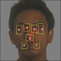
Figure 11.19 Pictorial structure. This face model consists of seven parts (red dots), which are connected together in a tree-like structure (red lines). The possible positions of each part are indicated by the yellow boxes. Although each part can take several hundred pixel positions, the MAP positions can be inferred efficiently by exploiting the tree-structure of the graph using a dynamic programming approach. Localizing facial features is a common element of many face recognition pipelines.

A second application is for fitting articulated models such as human bodies (Figure 11.20). These naturally have the form of a tree and so the structure is determined by the problem itself. Felzenszwalb and Huttenlocher (2005) developed a system of this sort in which each state w_n represented a part of the model (e.g., the right forearm). Each state could take K possible values representing different possible positions and shapes of the object part.

The image was preclassified into foreground and background using a background subtraction technique. The likelihood Pr(x_n|w=k) for a particular part position was evaluated using this binary image. In particular, the likelihood was chosen so that it increased if the area within the rectangle was considered foreground and the area surrounding it was considered background.

Unfortunately, MAP inference in this model is somewhat unreliable: a common failure mode is for more than one part of the body to become associated with the same part of the binary image. This is technically possible as the limbs may occlude each other, but it can also happen erroneously if one limb dominates and supports the rectangle model significantly more than the others. Felzenszwalb and Huttenlocher(2005) dealt with this problem by drawing samples from the posterior distribution Pr(w_1…N|x_1…N) over the positions of the parts of the model and using a more complex criterion to choose the most promising sample.

11.8.4 Segmentation

In Section 7.9.3, we considered segmentation as the problem of labeling pixels according to the object to which they belong. A different approach to segmentation is to infer the position of a closed contour that delineates two objects. In inference, the goal is usually to infer the positions of a set of points {w_n} on the boundary of this contour based on the image data x. As we update these points during an attempt to find the MAP solution, the contour moves across the image, and for this reason this type of model is referred to as an active contour or snake model.

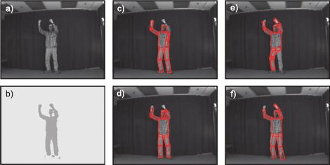
Figure 11.20 Pictorial structure for human body. a) Original image. b) After background subtraction. c-f) Four samples from the posterior distribution over part positions. Each part position is represented by a rectangle of fixed aspect ratio and characterized by its position, size, and angle. Adapted from Felzenszwalb and Huttenlocher (2005). ©2005 Springer.

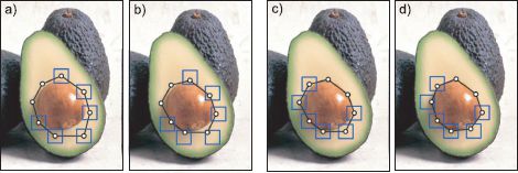
Figure 11.21 Segmentation using snakes. a) Two points are fixed, but the remaining points can take any position within their respective boxes. The posterior distribution favors positions that are on image contours (due to the likelihood term) and positions that are close to other points (due to the pairwise connections). b) Results of inference. c) Two other points are considered fixed. d) Result of inference. In this way, a closed contour in the image is identified. Adapted from Felzenszwalb and Zabih (2011). ©2011 IEEE.

Figure 11.21 shows an example of fitting this type of model. At each iteration, the positions {w_n} of all of the points except two are updated and can take any position within small region surrounding their previous position. The likelihood of taking a particular value w_n = k is high at positions in the image where the intensity changes rapidly (i.e., the edges) and low in constant regions. In addition, neighboring points are connected and have an attractive force: they are more likely to be close to one another. As usual, inference can be carried out using the dynamic programming method. During inference, the points tend to become closer together (due to their mutual attraction) but get stuck on the edge of an object.

In the full system, this process is repeated, but with a different pair of adjacent points chosen to be fixed at each step. Hence, the dynamic programming is a component step of a larger inference problem. As the inference procedure continues, the contour moves across the image and eventually fixes onto the boundary of an object. For this reason, these models are known as snakes or active contour models. They are considered in more detail in Chapter 17.

Discussion

In this chapter, we have considered models based on acyclic graphs (chains and trees). In Chapter 12, we will consider grid-based models that contain many loops. We will see that MAP inference is only tractable in a few special cases. In contrast to this chapter, we will also see a large difference between directed and undirected models.

Notes

Dynamic programming: Dynamic programming is used in many vision algorithms, including those where there is not necessarily a clear probabilistic interpretation. It is an attractive approach when it is applicable because of its speed, and some efforts have been made to improve this further (Raphael 2001). Interesting examples include image retargeting (Avidan and Shamir 2007), contour completion (sha’ashua and Ullman 1988), fitting of deformable templates (Amit and Kong 1996; Coughlan et al. 2000), shape matching (Basri et al. 1998), the computation of superpixels (Moore et al. 2008) and semantic labeling of scenes with tiered structure (Felzenszwalb and Veksler 2010) as well as the applications described in this chapter. Felzenszwalb and Zabih (2011) provide a recent review of dynamic programming and other graph algorithms in computer vision.

Stereo vision: Dynamic programming was variously applied to stereo vision by Baker and Binford (1981), Ohta and Kanade (1985) (who use a model based on edges) and Geiger et al. (1992) (who used a model based on intensities). Birchfield and Tomasi (1998) improved the speed by removing unlikely search nodes from the dynamic programming solution and introduced a mechanism that made depth discontinuities more likely where there was intensity variation. Torr and Criminisi (2004) developed a system that integrated dynamic programming with known constraints such as matched keypoints. Gong and Yang (2005) developed a dynamic programming algorithm that ran on a graphics processing unit (GPU). Kim et al. (2005) introduced a method for identifying disparity candidates at each pixel using spatial filters and a two-pass method that performed optimization both along and across the scanlines. Veksler (2005) used dynamic programming in a tree to solve for the whole image at once, and this idea has subsequently been used in a method based on line segments (Deng and Lin 2006). A recent quantitative comparison of dynamic programming algorithms in computer vision can be found in Salmen et al. (2009). Alternative approaches to stereo vision, which are not based on dynamic programming, are considered in Chapter 12.

Pictorial structures: Pictorial structures were originally introduced by Fischler and Erschlager (1973) but recent interest was stimulated by the work of Felzenszwalb and Huttenlocher (2005) who introduced efficient methods of inference based on dynamic programming. There have been a number of attempts to improve the appearance (likelihood) term of the model (Kumar et al. 2004; Eichner and Ferrari 2009; Andriluka et al. 2009; Felzenszwalb et al. 2010). Models that do not conform to a tree structure have also been introduced (Kumar et al. 2004; Sigal and Black 2006; Ren et al. 2005; Jiang and Martin 2008) and here alternative methods such as loopy propagation must be used for inference. These more general structures are particularly important for addressing problems associated with occlusions in human body models. Other authors have based their model on a mixture of trees (Everingham et al. 2006; Felzenszwalb et al. 2010). In terms of applications, Ramanan et al. (2008) have developed a notable system for tracking humans in video sequences based on pictorial structures, Everingham et al. (2006) have developed a widely used system for locating facial features, and Felzenszwalb et al. (2010) have presented a system that is used for detecting more general objects.

Hidden Markov models: Hidden Markov models are essentially chain-based models that are applied to quantities evolving in time. Good tutorials on the subject including details of how to learn them in the unsupervised case can be found in Rabiner (1989) and Ghahramani (2001). Their most common application in vision is for gesture recognition (Starner et al. 1998; Rigoll et al. 1998; and see Moni and Ali 2009 for a recent review), but they have also been used in other contexts such as modeling interactions of pedestrians (Oliver et al. 2000). Some recent work (e.g., Bor Wang et al. 2006) uses a related discriminative model for tracking objects in time known as a conditional random field (see Chapter 12).

Snakes: The idea of a contour evolving over the surface of an image is due to Kass et al. (1987). Both Amini et al. (1990) and Geiger et al. (1995) describe dynamic programming approaches to this problem. These models are considered further in Chapter 17.

Belief propagation: The sum-product algorithm (Kschischang et al. 2001) is a development of earlier work on belief propagation by Pearl (1988). The factor graph representation is due to Frey et al. (1997). The use of belief propagation for finding marginal posteriors and MAP solutions in graphs with loops has been investigated by Murphy et al. (1999) and Weiss and Freeman (2001), respectively. Notable applications of loopy belief propagation in vision include stereo vision (Sun et al. 2003) and superresolving images (Freeman et al. 2000). More information about belief propagation can be found in machine learning textbooks such as Bishop (2006), Barber (2012), and Koller and Friedman (2009).

Problems

11.1 Compute by hand the lowest possible cost for traversing the graph in Figure 11.22 using the dynamic programming method.

11.2 MAP inference in chain models can also be performed by running Djikstra’s algorithm on the graph in Figure 11.23, starting from the node on the left-hand side and terminating when we first reach the node on the right-hand side. If there are N variables, each of which takes K values, what is the best and worst case complexity of the algorithm? Describe a situation where Djikstra’s algorithm outperforms dynamic programming.

11.3 Consider the graphical model in Figure 11.24a. Write out the cost function for MAP estimation in the form of Equation 11.17. Discuss the difference between your answer and Equation 11.17.

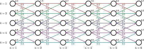
Figure 11.22 Dynamic programming example for Problem 11.1.

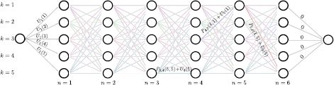
Figure 11.23 Graph construction for Problem 11.2. This is the same as the dynamic programming graph (Figure 11.3) except that: (i) there are two extra nodes at the start and the end of the graph. (ii) There are no vertex costs. (iii) The costs associated with the leftmost edges are U₁(k) and the costs associated with the rightmost edges are 0. The general edge cost for passing from label a and node n to label b at node n + 1 is given by P_{n, n + 1}(a, b) + U_n+1(b).

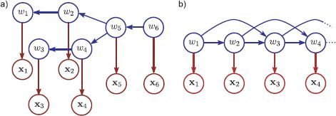
Figure 11.24 a) Graphical model for Problem 11.3. b) Graphical model for Problem 11.10. The unknown variables w₃, w₄,… in this model receive connections from the two preceding variables and so the graph contains loops.

11.4 Compute the solution (minimum cost path) to the dynamic programming problem on the tree in Figure 11.25 (which corresponds to the graphical model from Figure 11.6).

11.5 MAP inference for the chain model can be expressed as

Show that it is possible to compute this expression piecewise by moving the maximization terms through the summation sequence in a manner similar to that described in Section 11.4.1.

11.6 Develop an algorithm that can compute the marginal distribution for an arbitrary variable w_n in a chain model.

11.7 Develop an algorithm that computes the joint marginal distribution of any two variables w_m and w_n in a chain model.

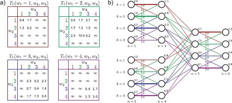
Figure 11.25 Dynamic programming example for Problem 11.4.

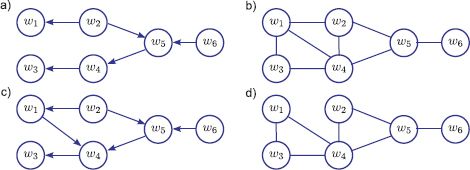
Figure 11.26 Graphical models for Problem 11.9.

11.8 Consider the following two distributions over three variables x₁, x₂, and x₃:

Draw (i) an undirected model and (ii) a factor graph for each distribution. What do you conclude?

11.9 Convert each of the graphical models in Figure 11.26 into the form of a factor graph. Which of the resulting factor graphs take the form of a chain?

11.10 Figure 11.24b shows a chain model in which each unknown variable w depends on its two predecessors. Describe a dynamic programming approach to finding the MAP solution. (Hint: You need to combine variables). If there are N variables in the chain and each takes K values, what is the overall complexity of your algorithm?

11.11 In the stereo vision problem, the solution was very poor when the pixels are treated independently (Figure 11.18a). Suggest some improvements to this method (while keeping the pixels independent).

11.12 Consider a variant on the segmentation application (Figure 11.21) in which we update all of the contour positions at once. The graphical model for this problem is a loop (i.e., a chain where there is also a edge between w_N and w₁). Devise an approach to finding the exact MAP solution in this model. If there are N variables each of which can take K values, what is the complexity of your algorithm?